HAL Id: hal-00369812
https://hal.archives-ouvertes.fr/hal-00369812v3
Preprint submitted on 9 Jul 2009
HAL is a multi-disciplinary open access
archive for the deposit and dissemination of
sci-entific research documents, whether they are
pub-lished or not. The documents may come from
teaching and research institutions in France or
abroad, or from public or private research centers.
L’archive ouverte pluridisciplinaire HAL, est
destinée au dépôt et à la diffusion de documents
scientifiques de niveau recherche, publiés ou non,
émanant des établissements d’enseignement et de
recherche français ou étrangers, des laboratoires
publics ou privés.
Volume and entropy of regular timed languages
Eugene Asarin, Aldric Degorre
To cite this version:
Eugene Asarin, Aldric Degorre.
Volume and entropy of regular timed languages.
2009.
�hal-00369812v3�
Volume and entropy of regular timed languages
Eugene Asarin1 and Aldric Degorre2 1 LIAFA, Universit´e Paris Diderot / CNRS
case 7014, 75205 Paris Cedex 13, France [email protected]
2 VERIMAG
,
Centre Equation, 2 av. de Vignate, 38610 Gi`eres, France [email protected]
Abstract. For timed languages, we define size measures: volume for lan-guages with a fixed finite number of events, and entropy (growth rate) as asymptotic measure for an unbounded number of events. These measures can be used for quantitative comparison of languages, and the entropy can be viewed as information contents of a timed language. For languages accepted by deterministic timed automata, we give exact formulas for volumes. Next, we characterize the entropy, using methods of functional analysis, as a logarithm of the leading eigenvalue (spectral radius) of a positive integral operator. We devise several methods to compute the entropy: a symbolical one for so-called “11
2-clock” automata, and two
nu-merical ones: one using techniques of functional analysis, another based on discretization. We give an information-theoretic interpretation of the entropy in terms of Kolmogorov complexity.
1
Introduction
Since early 90s, timed automata and timed languages are extensively used for modelling and verification of real-time systems, and thoroughly explored from a theoretical standpoint. However, two important, and closely related, aspects have never been addressed: quantitative analysis of the size of these languages and of information content of timed words. In this paper, we formalize and solve these problems for a large subclass of timed automata.
Recall that a timed word describes a behaviour of a system, taking into account delays between events. For example, 2𝑎3.11𝑏 means that an event 𝑎 happened 2 time units after the system start, and 𝑏 happened 3.11 time units after 𝑎. A timed language, which is just a set of timed words, may represent all such potential behaviours. Our aim is to measure the size of such a language. For a fixed number 𝑛 of events, we can consider the language as a subset of 𝛴𝑛× IR𝑛
(that is of several copies of the space IR𝑛). A natural measure in this case is just Euclidean volume 𝑉𝑛 of this subset. When the number of events is not fixed, we
can still consider for each 𝑛 all the timed words with 𝑛 events belonging to the language and their volume 𝑉𝑛. It turns out that in most cases 𝑉𝑛asymptotically
The information-theoretic meaning of ℋ can be stated as follows: for a small 𝜀, if the delays are measured with a finite precision 𝜖, then using the words of the language 𝐿 with entropy ℋ one can transmit ℋ + log(1/𝜀) bits of information per event (see Thms. 7-8 below for a formalization in terms of Kolmogorov complexity).
There can be several potential applications of these notions:
– The most direct one is capacity estimation for an information transmission channel or for a time-based information flow.
– When one overapproximates a timed language 𝐿1 by a simpler timed
lan-guage 𝐿2(using, for example, some abstractions as in [1]), it is important to
assess the quality of the approximation. Comparison of entropies of 𝐿1 and
𝐿2provides such an assessment.
– In model-checking of timed systems, it is often interesting to know the size of the set of all behaviours violating a property or of a subset of those presented as a counter-example by a verification tool.
In this paper, we explore, and partly solve the following problems: given a prefix-closed timed language accepted by a timed automaton, find the volume 𝑉𝑛 of the set of accepted words of a given length 𝑛 and the entropy ℋ of the
whole language.
Related Work. Our problems and techniques are inspired by works concerning the entropy of finite-state languages (cf. [2]). There the cardinality of the set 𝐿𝑛
of all elements of length 𝑛 of a prefix-closed regular language also behaves as 2𝑛ℋfor some entropy ℋ. This entropy can be found as logarithm of the spectral
radius of adjacency matrix of reachable states of 𝒜.3 The main technical tool
used to compute the entropy of finite automata is the Perron-Frobenius theory for positive matrices, and, in this paper, in a first approach we will use its extensions to infinite-dimensional operators [3]. In a second approach, we also propose to reduce our problem by discretization to entropy computation for some discrete automata.
In [4, 5] probabilities of some timed languages and densities in the clock space are computed. Our formulae for fixed-length volumes can be seen as specializa-tion of these results to uniform measures. As for unbounded languages, they use stringent condition of full simultaneous reset of all the clocks at most every 𝑘 steps, and under such a condition, they provide a finite stochastic class graph that allows computing various interesting probabilities. We use a much weaker hypothesis (every clock to be reset at most every 𝐷 steps, but these resets need not be simultaneous), and we obtain only the entropy.
In [6] probabilities of LTL properties of one-clock timed automata (over in-finite timed words) are computed using Markov chains techniques. It would be interesting to try to adapt our methods to this kind of problems.
Last, our studies of Kolmogorov complexity of rational elements of timed languages, relating this complexity to the entropy of the language, remind of
earlier works on complexity of rational approximations of continuous functions [7, 8], and those relating complexity of trajectories to the entropy of dynamical systems [9, 8].
Paper Organization This paper is organized as follows. In Sect. 2 we define volumes of fixed-length timed languages and entropy of unbounded-length timed languages. We identify a subclass of deterministic timed automata, whose vol-umes and entropy are considered in the rest of the paper, and a normal form for such automata. Finally, we provide an algorithm for computing the volumes of languages of such automata. In Sect. 3 we define a functional space associated to a timed automaton and a positive operator on this space. We rephrase the formulas for the volume in terms of this operator. Next, we state the main result of the paper: a characterization of the entropy as the logarithm of the spectral radius of this operator. Such a characterization could seem too abstract but later on, in sections 4-5 we give three practical procedures for approximate comput-ing this spectral radius. First, we show how to solve the eigenvector equation symbolically in case of timed automata with 121 clocks defined below. Next, for general timed automata we apply a “standard” iterative procedure from [3] and thus obtain an upper and a lower bound for the spectral radius/entropy. These bounds become tighter as we make more iterations. Last, in Sect. 5, also for general timed automata, we devise a procedure that provides upper and lower bounds of the entropy by discretization of the timed automaton. In the same section, and using the same method, we give an interpretation of the entropy of timed regular languages in terms of Kolmogorov complexity. We conclude the paper by some final remarks in Sect. 7. Throughout the paper, the concepts and the techniques are illustrated by several running examples.
2
Problem statement
2.1 Geometry, Volume and Entropy of Timed Languages
A timed word of length 𝑛 over an alphabet 𝛴 is a sequence 𝑤 = 𝑡1𝑎1𝑡2. . . 𝑡𝑛𝑎𝑛,
where 𝑎𝑖 ∈ 𝛴, 𝑡𝑖 ∈ IR and 0 ≤ 𝑡𝑖 (notice that this definition rules out timed
words ending by a time delay). Here 𝑡𝑖 represents the delay between the events
𝑎𝑖−1 and 𝑎𝑖. With such a timed word 𝑤 of length 𝑛 we associate its untiming
𝜂(𝑤) = 𝑎1, . . . , 𝑎𝑛∈ 𝛴𝑛 (which is just a word), and its timing which is a point
𝜃(𝑤) = (𝑡1, . . . , 𝑡𝑛) in IR𝑛. A timed language 𝐿 is a set of timed words. For a
fixed 𝑛, we define the 𝑛-volume of 𝐿 as follows: 𝑉𝑛(𝐿) =
∑
𝑣∈𝛴𝑛
Vol{𝜃(𝑤) ∣ 𝑤 ∈ 𝐿, 𝜂(𝑤) = 𝑣},
where Vol stands for the standard Euclidean volume in IR𝑛. In other words, we sum up over all the possible untimings 𝑣 of length 𝑛 the volumes of the corresponding sets of delays in IR𝑛. In case of regular timed languages, these sets are polyhedral, and hence their volumes (finite or infinite) are well-defined.
We associate with every timed language a sequence of 𝑛-volumes 𝑉𝑛. We
will show in Sect. 2.5 that, for languages of deterministic timed automata, 𝑉𝑛
is a computable sequence of rational numbers. However, we would like to find a unique real number characterizing the asymptotic behaviour of 𝑉𝑛 as 𝑛 → ∞.
Typically, 𝑉𝑛 depends approximately exponentially on 𝑛. We define the entropy
of a language as the rate of this dependence.
Formally, for a timed language 𝐿 we define its entropy as follows4(all
loga-rithms in the paper are base 2):
ℋ(𝐿) = lim sup
𝑛→∞
log 𝑉𝑛
𝑛 .
Remark 1. Many authors consider a slightly different kind of timed words: se-quences 𝑤 = (𝑎1, 𝑑1), . . . , (𝑎𝑛, 𝑑𝑛), where 𝑎𝑖∈ 𝛴, 𝑑𝑖∈ IR and 0 ≤ 𝑑1≤ ⋅ ⋅ ⋅ ≤ 𝑑𝑛,
with 𝑑𝑖representing the date of the event 𝑎𝑖. This definition is in fact isomorphic
to ours by a change of variables: 𝑡1 = 𝑑1 and 𝑡𝑖 = 𝑑𝑖− 𝑑𝑖−1 for 𝑖 = 2..𝑛. It is
important for us that this change of variables preserves the 𝑛-volume, since it is linear and its matrix has determinant 1. Therefore, choosing date (𝑑𝑖) or delay
(𝑡𝑖) representation has no influence on language volumes (and entropy). Due to
the authors’ preferences (justified in [10]), delays will be used in the sequel.
2.2 Three Examples 𝒜1 p 𝑎, 𝑥 ∈ [2; 4]/𝑥 := 0 𝑏, 𝑥 ∈ [3; 10]/𝑥 := 0 𝒜2 p q 𝑎, 𝑥 ∈ [0; 4] 𝑏, 𝑥 ∈ [2; 4]/𝑥 := 0 𝒜3 p q 𝑎, 𝑥 ∈ [0; 1]/𝑥 := 0 𝑏, 𝑦 ∈ [0; 1]/𝑦 := 0
Fig. 1.Three simple timed automata 𝒜1, 𝒜2, 𝒜3
To illustrate the problem consider the languages recognized by three timed automata on Fig. 1. Two of them can be analysed directly, using definitions and common sense. The third one resists naive analysis, it will be used to illustrate more advanced methods throughout the paper.
Rectangles. Consider the timed language defined by the expression 𝐿1= ([2; 4]𝑎 + [3; 10]𝑏)∗,
4
In fact, due to Assumption A2 below, the languages we consider in the paper are prefix-closed, and lim sup is in fact a lim. This will be stated formally in Cor. 1.
recognized by 𝒜1 of Fig. 1.
For a given untiming 𝑤 ∈ {𝑎, 𝑏}𝑛 containing 𝑘 letters 𝑎 and 𝑛 − 𝑘 letters 𝑏,
the set of possible timings is a rectangle in IR𝑛 of a volume 2𝑘7𝑛−𝑘 (notice that there are 𝐶𝑘
𝑛 such untimings). Summing up all the volumes, we obtain
𝑉𝑛(𝐿1) = 𝑛
∑
𝑘=0
𝐶𝑛𝑘2𝑘7𝑛−𝑘= (2 + 7)𝑛= 9𝑛,
and the entropy ℋ(𝐿1) = log 9 ≈ 3.17.
A Product of Trapezia. Consider the language defined by the automaton
𝒜2 on Fig. 1, that is containing words of the form 𝑡1𝑎𝑠1𝑏𝑡2𝑎𝑠2𝑏 . . . 𝑡𝑘𝑎𝑠𝑘𝑏 such
that 2 ≤ 𝑡𝑖+ 𝑠𝑖≤ 4. Since we want prefix-closed languages, the last 𝑠𝑘𝑏 can be
omitted.
For an even 𝑛 = 2𝑘 the only possible
un-s
2 4
2 4 t
Fig. 2.Timings (𝑡𝑖, 𝑠𝑖) for 𝒜2.
timing is (𝑎𝑏)𝑘. The set of timings in IR2𝑘is a
Cartesian product of 𝑘 trapezia 2 ≤ 𝑡𝑖+ 𝑠𝑖≤
4. The surface of each trapezium equals 𝑆 = 42/2 − 22/2 = 6, and the volume 𝑉
2𝑘(𝐿2) =
6𝑘. For an odd 𝑛 = 2𝑘 + 1 the same product
of trapezia is combined with an interval 0 ≤ 𝑡𝑘+1 ≤ 4, hence the volume is 𝑉2𝑘+1(𝐿2) =
6𝑘⋅ 4. Thus the entropy ℋ(𝐿
2) = log 6/2 ≈
1.29.
Our Favourite Example. The language recognized by the automaton 𝒜3 on
Fig. 1 contains the words of the form 𝑡1𝑎𝑡2𝑏𝑡3𝑎𝑡4𝑏 . . . with 𝑡𝑖+ 𝑡𝑖+1 ∈ [0; 1].
Notice that the automaton has two clocks that are never reset together. The geometric form of possible untimings in IR𝑛is defined by overlapping constraints 𝑡𝑖+ 𝑡𝑖+1∈ [0; 1].
It is not so evident how to compute the volume of this polyhedron. A sys-tematic method is described below in Sect. 2.5. An ad hoc solution would be to integrate 1 over the polyhedron, and to rewrite this multiple integral as an iterated one. The resulting formula for the volume is
𝑉𝑛(𝐿3) = ∫ 1 0 𝑑𝑡1 ∫ 1−𝑡1 0 𝑑𝑡2 ∫ 1−𝑡2 0 𝑑𝑡3. . . ∫ 1−𝑡𝑛−1 0 𝑑𝑡𝑛.
This gives the sequence of volumes: 1;1 2; 1 3; 5 24; 2 15; 61 720; 17 315; 277 8064; . . .
2.3 Subclasses of Timed Automata
In the rest of the paper, we compute volumes and entropy for regular timed languages recognized by some subclasses of timed automata (TA). We assume that the reader is acquainted with timed automata; otherwise, we refer her or him to [11] for details. Here we only fix notations for components of timed automata and state several requirements they should satisfy. Thus a TA is a tuple 𝒜 = (𝑄, 𝛴, 𝐶, 𝛥, 𝑞0). Its elements are respectively the set of locations, the
alphabet, the set of clocks, the transition relation, and the initial location (we do not need to specify accepting states due to A2 below, neither we need any invariants). A generic state of 𝒜 is a pair (𝑞, x) of a control location and a vector of clock values. A generic element of 𝛥 is written as 𝛿 = (𝑞, 𝑎, 𝔤, 𝔯, 𝑞′) meaning
a transition from 𝑞 to 𝑞′ with label 𝑎, guard 𝔤 and reset 𝔯. We spare the reader
the definitions of a run of 𝒜 and of its accepted language.
Several combinations of the following Assumptions will be used in the sequel:
A1. The automaton 𝒜 is deterministic5.
A2. All its states are accepting.
A3. Guards are rectangular (i.e. conjunctions of constraints 𝐿𝑖≤ 𝑥𝑖≤ 𝑈𝑖, strict
inequalities are also allowed). Every guard upper bounds at least one clock. A4. There exists a 𝐷 ∈ IN such that on every run segment of 𝐷 transitions,
every clock is reset at least once.
A5. There is no punctual guards, that is in any guard 𝐿𝑖< 𝑈𝑖.
Below we motivate and justify these choices:
A1: Most of known techniques to compute entropy of untimed regular languages work on deterministic automata. Indeed, these techniques count paths in the automaton, and only in the deterministic case their number coincides with the number of accepted words. The same is true for volumes in timed automata. R. Lanotte pointed out to the authors that any TA satisfying A4 can be determinized.
A2: Prefix-closed languages are natural in the entropy context, and somewhat easier to study. These languages constitute the natural model for the set of behaviours of causal systems.
A3: If a guard of a feasible transition is infinite, the volume becomes infinite. We conclude that A3 is unavoidable and almost not restrictive.
5
That is any two transitions with the same source and the same label have their guards disjoint.
A4: We use this variant of non-Zenoness condition several times in our proofs and constructions. As the automaton of Fig. 3 shows, if we omit this as-sumption some anomalies can occur.
The language of this automaton is
𝑎, 𝑥 ∈ [0; 1] Fig. 3. An automaton without resets 𝐿 = {𝑡1𝑎 . . . 𝑡𝑛𝑎 ∣ 0 ≤ ∑ 𝑡𝑖≤ 1},
and 𝑉𝑛 is the volume of an 𝑛-dimensional
sim-plex defined by the constraints 0 ≤ ∑ 𝑡𝑖 ≤ 1,
and 0 ≤ 𝑡𝑖. Hence 𝑉𝑛 = 1/𝑛! which decreases
faster than any exponent, which is too fine to be distinguished by our methods. Assumption A4 rules out such anomalies. This assumption is also the most difficult to check. A possible way would be to explore all simple cycles in the region graph and to check that all of those reset every clock.
A5: While assumptions A1-A4 can be restrictive, we always can remove the transitions with punctual guards from any automaton, without changing the volumes 𝑉𝑛. Hence, A5 is not restrictive at all, as far as volumes are
considered. In Sect. 6 we do not make this assumption.
2.4 Preprocessing Timed Automata
In order to compute volumes 𝑉𝑛 and entropy ℋ of the language of a nice TA,
we first transform this automaton into a normal form, which can be considered as a (timed) variant of the region graph, the quotient of the TA by the region equivalence relation defined in [11].
We say that a TA 𝒜 = (𝑄, 𝛴, 𝐶, 𝛿, 𝑞0) is in a region-split form if A1, A2, A4
and the following properties hold:
B1. Each location and each transition of 𝒜 is visited by some run starting at (𝑞0, 0).
B2. For every location 𝑞 ∈ 𝑄 a unique clock region r𝑞 (called its entry region)
exists, such that the set of clock values with which 𝑞 is entered is exactly r𝑞. For the initial location 𝑞0, its entry region is the singleton {0}.
B3. The guard 𝔤 of every transition 𝛿 = (𝑞, 𝑎, 𝔤, 𝔯, 𝑞′) ∈ 𝛥 is just one clock
region.
Notice, that B2 and B3 imply that 𝔯(𝔤) = r𝑞′ for every 𝛿.
Proposition 1. Given a nice TA 𝒜, a region-split TA 𝒜′ accepting the same
language can be constructed6.
6 Notice that due to A3 all the guards of original automaton are bounded w.r.t. some
clock. Hence, the same holds for smaller (one-region) guards of 𝒜′, that is the infinite region [𝑀 ; ∞)∣𝐶∣never occurs as a guard.
Proof (sketch). Let 𝒜 = (𝑄, 𝛴, 𝐶, 𝛥, 𝑞0) be a nice TA and let Reg be the set
of its regions. The region-split automaton 𝒜′ = (𝑄′, 𝛴, 𝐶, 𝛥′, 𝑞′
0) can be
con-structed as follows:
1. Split every state 𝑞 into substates corresponding to all possible entry regions. Formally, just take 𝑄′= 𝑄 × Reg.
2. Split every transition from 𝑞 to 𝑞′ according to two clock regions: one for
the clock values when 𝑞 is entered, another for clock values when 𝑞 is left. Formally, for every 𝛿 = (𝑞, 𝑎, 𝔤, 𝔯, 𝑞′) of 𝒜, and every two clock regions r and
r′ such that r′ is reachable from r by time progress, and r′ ⊂ 𝔤, we define a
new transition of 𝒜′
𝛿′rr′ = ((𝑞, r), 𝑎, x ∈ r
′, 𝔯, (𝑞′, 𝔯(r′))) .
3. Take as initial state 𝑞′
0= (𝑞0, {0}).
4. Remove all the states and transitions not reachable from the initial state. ⊓⊔ We could work with the region-split automaton, but it has too many useless (degenerate) states and transitions, which do not contribute to the volume and the entropy of the language. This justifies the following definition: we say that a region-split TA is fleshy if the following holds:
B4. For every transition 𝛿 its guard 𝔤 has no constraints of the form 𝑥 = 𝑐 in its definition.
Proposition 2. Given a region-split TA 𝒜 accepting a language 𝐿, a fleshy region-split nice TA 𝒜′ accepting a language 𝐿′ ⊂ 𝐿 with 𝑉
𝑛(𝐿′) = 𝑉𝑛(𝐿) and
ℋ(𝐿′) = ℋ(𝐿) can be constructed.
Proof (sketch). The construction is straightforward: 1. Remove all non-fleshy transitions.
2. Remove all the states and transitions that became unreachable.
Inclusion 𝐿′ ⊂ 𝐿 is immediate. Every path in 𝒜 (of length 𝑛) involving a
non-fleshy (punctual) transition corresponds to the set of timings in IR𝑛 which is degenerate (its dimension is smaller than 𝑛), hence it does not contribute to
𝑉𝑛. ⊓⊔
From now on, we suppose w.l.o.g. that the automaton 𝒜 is in a fleshy region-split form (see Fig. 4).
2.5 Computing Volumes
Given a timed automaton 𝒜 satisfying A1-A3, we want to compute 𝑛-volumes 𝑉𝑛
of its language. In order to obtain recurrent equations on these volumes, we need to take into account all possible initial locations and clock configurations. For every state (𝑞, x), let 𝐿(𝑞, x) be the set of all the timed words corresponding to the runs of the automaton starting at this state, let 𝐿𝑛(𝑞, x) be its sublanguage
𝑝 𝑥 = 0 𝑞 𝑥 ∈ (0; 1) (0; 1) 𝑞 𝑥 ∈ (1; 2) 𝑞 𝑥 ∈ (2; 3) 𝑞 𝑥 ∈ (3; 4) (1; 2)(2; 3) 𝑎, 𝑥 ∈ (3; 4) 𝑏, 𝑥 ∈ (2; 3)/𝑥 := 0 𝑏, 𝑥 ∈ (3; 4)/𝑥 := 0 𝑝 𝑥 ∈ (0; 1) 𝑦 = 0 𝑞 𝑥 = 0 𝑦 ∈ (0; 1) 𝑎, 𝑥 ∈ (0; 1)/𝑥 := 0 𝑏, 𝑦 ∈ (0; 1)/𝑦 := 0 𝑝 𝑥 = 0 𝑦 = 0 𝑎, 𝑥 ∈ (0; 1)/𝑥 := 0
Fig. 4.Fleshy region-split forms of automata 𝒜2and 𝒜3 from Fig. 1. An entry region
is drawn at each location.
consisting of its words of length 𝑛, and 𝑣𝑛(𝑞, x) the volume of this sublanguage.
Hence, the quantity we are interested in, is a value of 𝑣𝑛 in the initial state:
𝑉𝑛 = 𝑣𝑛(𝑞0, 0).
By definition of runs of a timed automaton, we obtain the following language equations: 𝐿0(𝑞, x) = 𝜀; 𝐿𝑘+1(𝑞, x) = ∪ (𝑞,𝑎,𝔤,𝔯,𝑞′)∈𝛥 ∪ 𝜏 :x+𝜏 ∈𝔤 𝜏 𝑎𝐿𝑘(𝑞′, 𝔯(x + 𝜏 )).
Since the automaton is deterministic, the union over transitions (the first∪ in the formula) is disjoint. Hence, it is easy to pass to volumes:
𝑣0(𝑞, x) = 1; (1) 𝑣𝑘+1(𝑞, x) = ∑ (𝑞,𝑎,𝔤,𝔯,𝑞′)∈𝛥 ∫ 𝜏 :x+𝜏 ∈𝔤 𝑣𝑘(𝑞′, 𝔯(x + 𝜏 )) 𝑑𝜏. (2)
Remark that for a fixed location 𝑞, and within every clock region, as defined in [11], the integral over 𝜏 : x + 𝜏 ∈ 𝔤 can be decomposed into several ∫𝑢
𝑙 with
bounds 𝑙 and 𝑢 either constants or of the form 𝑐 − 𝑥𝑖 with 𝑐 an integer and 𝑥𝑖a
clock variable.
These formulas lead to the following structural description of 𝑣𝑛(𝑞, x), which
can be proved by a straightforward induction.
Lemma 1. The function 𝑣𝑛(𝑞, x) restricted to a location 𝑞 and a clock region
can be expressed by a polynomial of degree 𝑛 with rational coefficients in variables x.
Thus in order to compute the volume 𝑉𝑛 one should find by symbolic
inte-gration polynomial functions 𝑣𝑘(𝑞, x) for 𝑘 = 0..𝑛, and finally compute 𝑣𝑛(𝑞0, 0).
Theorem 1. For a timed automaton 𝒜 satisfying A1-A3, the volume 𝑉𝑛 is a
3
Operator Approach
In this central section of the paper, we develop an approach to volumes and entropy of languages of nice timed automata based on functional analysis, first introduced in [12].
We start in 3.1 by identifying a functional space ℱ containing the volume functions 𝑣𝑛. Next, we show that these volume functions can be seen as iterates
of some positive integral operator 𝛹 on this space applied to the unit function (Sect. 3.2). We explore some elementary properties of this operator in 3.3. This makes it possible to apply in 3.4 the theory of positive operators to 𝛹 and to deduce the main theorem of this paper stating that the entropy equals the logarithm of the spectral radius of 𝛹 .
3.1 The Functional Space of a TA
In order to use the operator approach we first identify the appropriate functional space ℱ containing volume functions 𝑣𝑛.
We define 𝑆 as the disjoint union of all the entry regions of all the states of 𝒜. Formally, 𝑆 = {(𝑞, x) ∣ x ∈ r𝑞}. The elements of the space ℱ are bounded
continuous functions from 𝑆 to IR. The uniform norm ∥𝑢∥ = sup𝜉∈𝑆∣𝑢(𝜉)∣ can be
defined on ℱ , yielding a Banach space structure. We can compare two functions in ℱ pointwise, thus we write 𝑢 ≤ 𝑣 if ∀𝜉 ∈ 𝑆 : 𝑢(𝜉) ≤ 𝑣(𝜉). For a function 𝑓 ∈ ℱ we sometimes denote 𝑓 (𝑝, 𝑥) by 𝑓𝑝(𝑥). Thus, any function 𝑓 ∈ ℱ can be seen as
a finite collection of functions 𝑓𝑝 defined on entry regions r𝑝 of locations of 𝒜.
The volume functions 𝑣𝑛 (restricted to 𝑆) can be considered as elements of ℱ .
3.2 Volumes Revisited
Let us consider again the recurrent formula (2). It has the form 𝑣𝑘+1 = 𝛹 𝑣𝑘,
where 𝛹 is the positive linear operator on ℱ defined by the equation:
𝛹 𝑓 (𝑞, x) = ∑
(𝑞,𝑎,𝔤,𝔯,𝑞′)∈𝛥
∫
x+𝜏 ∈𝔤
𝑓 (𝑞′, 𝔯(x + 𝜏 )) 𝑑𝜏. (3)
We have also 𝑣0= 1. Hence 𝑣𝑛 = 𝛹𝑛1, and the problem of computing volumes
and entropy is now phrased as studying iterations of a positive bounded linear operator 𝛹 on the functional space ℱ . The theory of positive operators guaran-tees, that under some hypotheses, 𝑣𝑛is close in direction to a positive eigenvector
𝑣∗ of 𝛹 , corresponding to its leading eigenvalue 𝜌. Moreover, values of 𝑣 𝑛 will
grow/decay exponentially like 𝜌𝑛. In the sequel, we refer to the book [3] when a
result concerning positive operators is needed.
3.3 Exploring the Operator 𝜳
Let us first state some elementary properties of this operator, starting by rewrit-ing (3) as an operator on ℱ and separatrewrit-ing all its summands.
(𝛹 𝑓 )𝑞(x) =
∑
𝛿=(𝑞,...,𝑞′)∈𝛥
For 𝛿 = (𝑞, 𝑎, 𝔤, 𝔯, 𝑞′) the operator 𝜓
𝛿 acts from the space 𝐶(r𝑞′) of bounded
continuous functions on the target region to the space 𝐶(r𝑞) of functions on the
source region. It is defined by the integral: 𝜓𝛿𝑓 (x) =
∫
x+𝜏 ∈𝔤
𝑓 (𝔯(x + 𝜏 )) 𝑑𝜏. Iterating (4), we obtain a formula for powers of operator 𝛹
(𝛹𝑘𝑓 )𝑝(x) =
∑
𝛿1...𝛿𝑘 from𝑝to 𝑝′
(𝜓𝛿1. . . 𝜓𝛿𝑘𝑓𝑝′)(x). (5)
Now we need some results on the iterations of 𝜓𝛿. For this, first we state
some useful properties of 𝜓𝛿 and its partial derivatives:
Proposition 3. For any 𝑓 ∈ 𝐶(r𝑞):
1. If 𝑓 ≥ 0 and 𝑓 is not identically 0 then 𝜓𝛿𝑓 is not identically 0.
2. ∥𝜓𝛿𝑓 ∥ ≤ ∥𝑓 ∥ (in other words, ∥𝜓𝛿∥ ≤ 1).
3. If 𝛿 resets 𝑥𝑖 then 𝜓𝛿𝑓 is continuously differentiable by 𝑥𝑖 and ∥∂𝑥∂𝑖𝜓𝛿𝑓 ∥ ≤
2∥𝑓 ∥
4. If 𝛿 does not reset 𝑥𝑖 and 𝑓 is continuously differentiable by 𝑥𝑖, then 𝜓𝛿𝑓 is
continuously differentiable by 𝑥𝑖 and ∥∂𝑥∂𝑖𝜓𝛿𝑓 ∥ ≤ 2∥𝑓 ∥ + ∥∂𝑥∂𝑖𝑓 ∥.
Proof.
(1) Let x1∈ r𝑞′ be such that 𝑓 (x1) > 0.
By B2 and B3, we know that there exists x2 ∈ 𝔤 such that 𝔯(x2) = x1. As
x2∈ 𝔤, there also exists 𝑥3∈ r𝑞 and 𝜏 ∈ IR≥0 verifying x2= x3+ 𝜏0.
Furthermore, because 𝛿 is fleshy, there exists 𝜏1 and 𝜏2, 𝜏1 < 𝜏2, such that
for every 𝜏 ∈ [𝜏1, 𝜏2], 𝑥3+ 𝜏 ∈ 𝔤.
Put together, the integration interval of 𝜓𝛿𝑓 (x3) = ∫x
3+𝜏 ∈𝔤𝑓 (𝔯(x3+ 𝜏 )) 𝑑𝜏
contains a value 𝜏0, for which the integrated function is positive, and includes
[𝜏1, 𝜏2], thus is neither empty nor a singleton. The integrated function being
non-negative and continuous, its integral, 𝜓𝛿𝑓 (x3), is positive.
(2) In 𝜓𝛿𝑓 (x) = ∫x+𝜏 ∈𝔤𝑓 (𝔯(x + 𝜏 )) 𝑑𝜏 , we estimate ∣𝑓 (⋅)∣ from above by the
constant ∥𝑓 ∥ and the length of the integration interval by 1, as it is included in the region 𝔤. This gives us the requested bound.
(3) As 𝔯 resets 𝑥𝑖, 𝑓 (𝑞′, 𝔯(x + 𝜏 )) does not depend on 𝑥𝑖, and thus 𝜓𝛿(𝑞, 𝑥) =
∫
x+𝜏 ∈𝔤𝑓 (𝑞′, 𝔯(x + 𝜏 )) 𝑑𝜏 is differentiable by 𝑥𝑖. Its derivative is
∂ ∂𝑥𝑖 𝜓𝛿𝑓 (𝑞, x) = ∂ ∂𝑥𝑖 ∫ x+𝜏 ∈𝔤 𝑓 (𝑞′, 𝔯(x + 𝜏 )) 𝑑𝜏 (6) = ±(𝑓 (𝑞′, 𝔯(x + 𝜏 𝑚𝑎𝑥) − 𝑓 (𝑞′, 𝔯(x + 𝜏𝑚𝑖𝑛))). (7)
The choice of + or − sign in the line (7) and the bounds 𝜏𝑚𝑎𝑥and 𝜏𝑚𝑖𝑛 depend
on the form of the guard.
First, observe that the latter term is a sum of continuous functions and, as such, is continuous. Furthermore, this term is bounded in absolute value by 2∥𝑓 ∥. Thus, we prove ∣ ∂
(4) As 𝑓 is differentiable by 𝑥𝑖, then so is 𝜓𝛿𝑓 (𝑞, x) =∫x+𝜏 ∈𝔤𝑓 (𝑞′, 𝔯(x + 𝜏 )) 𝑑𝜏 .
Let us differentiate it: ∂ ∂𝑥𝑖 𝜓𝛿𝑓 (𝑞, x) = ∂ ∂𝑥𝑖 ∫ x+𝜏 ∈𝔤 𝑓 (𝑞′, 𝔯(x + 𝜏 )) 𝑑𝜏 ∂ ∂𝑥𝑖 𝜓𝛿𝑓 (𝑞, x) = ± (𝑓 (𝑞′, 𝔯(x + 𝜏𝑚𝑎𝑥) − 𝑓 (𝑞′, 𝔯(x + 𝜏𝑚𝑖𝑛))) + ∫ x+𝜏 ∈𝔤 ∂ ∂𝑥𝑖𝑓 (𝑞 ′, 𝔯(x + 𝜏 )) 𝑑𝜏.
The resulting expression is still continuous in 𝑥𝑖. Indeed the newly added
term in the last equality is an integral of a continuous function that does not depend on 𝑥𝑖 on an interval that continuously depends on 𝑥𝑖.
We already stated that ∣(𝑓 (𝑞′, 𝔯(x + 𝜏
𝑚𝑎𝑥) − 𝑓 (𝑞′, 𝔯(x + 𝜏𝑚𝑖𝑛)))∣ is smaller
than 2∥𝑓 ∥. Also in∫
x+𝜏 ∈𝔤 ∂ ∂𝑥𝑖𝑓 (𝑞
′, 𝔯(x + 𝜏 )) 𝑑𝜏 , we can estimate the integrated
function from above by the norm ∥∂𝑥∂𝑖𝑓 ∥. As the integration interval is smaller than 1, the integral is smaller than this norm too. Hence, the required inequality
holds: ∣∂𝑥∂𝑖𝜓𝛿𝑓 (𝑞, x)∣ ≤ 2∥𝑓 ∥ + ∥∂𝑥∂𝑖𝑓 ∥. ⊓⊔
Now, we can prove the following result on the powers of 𝛹 . Proposition 4. Consider operator 𝛹 .
1. If 𝑓 ≥ 0 is not zero on 𝑝′ and there is a path of length 𝑘 from 𝑝 to 𝑝′ then
𝛹𝑘𝑓 is not identically zero on 𝑝.
2. For 𝐷 defined in assumption A4 there exists a constant 𝐸 ∈ IR such that for any 𝑓 ∈ ℱ the following estimate hold:
∀𝑖 : ∂ ∂𝑥𝑖 𝛹𝐷𝑓 ≤ 𝐸∥𝑓 ∥. Proof.
(1) This is a straightforward induction using (5) and Prop. 3-1. (2) For some 𝑥𝑖, and a location 𝑝, the following equality holds:
∂ ∂𝑥𝑖 (𝛹𝐷𝑓 )𝑝(x) = ∑ 𝛿1...𝛿𝐷 from 𝑝to𝑝′ ∂ ∂𝑥𝑖 (𝜓𝛿1. . . 𝜓𝛿𝐷𝑓𝑝′)(x).
Let us consider one term of this sum corresponding to one path. By hypoth-esis, in this path, there is a first transition 𝛿𝑘, 1 ≤ 𝑘 ≤ 𝐷, such that 𝛿𝑘 resets
𝑥𝑖.
By Prop. 3-3, 𝜓𝛿𝑘. . . 𝜓𝛿𝐷𝑓𝑝′is continuously differentiable by 𝑥𝑖. By induction
and using Prop. 3-4, it follows that 𝜓𝛿1. . . 𝜓𝛿𝑘. . . 𝜓𝛿𝐷𝑓𝑝′ is also continuously
differentiable by 𝑥𝑖.
Now we differentiate this term. For every 𝑗, 1 ≤ 𝑗 ≤ 𝐷, iterating Prop. 3-2 𝐷 − 𝑗 times, we obtain
𝜓𝛿𝑗. . . 𝜓𝛿𝐷𝑓𝑝′
∂ ∂𝑥𝑖𝜓𝛿𝑘. . . 𝜓𝛿𝐷𝑓𝑝′
≤ 2 ∥𝑓 ∥. It follows by induction on the path, using Prop. 3-4, that ∂ ∂𝑥𝑖𝜓𝛿1. . . 𝜓𝛿𝑘. . . 𝜓𝛿𝐷𝑓𝑝′ ≤ 2𝑘 ∥𝑓 ∥.
Now, if we come back to the sum, we have, at least, the following bound: ∂ ∂𝑥𝑖(𝛹 𝐷𝑓 ) 𝑝 ≤ 2𝑑
𝐷𝐷∥𝑓 ∥ (𝑑: maximal degree of the underlying graph of 𝛥),
which is true for every 𝑝, therefore ∥∂𝑥∂𝑖𝛹𝐷𝑓 ∥ ≤ 2𝑑𝐷𝐷∥𝑓 ∥. ⊓⊔
Now we are ready to prove the following important property of 𝛹 : Theorem 2. The operator 𝛹𝐷 is compact on ℱ .
Proof. Consider ℬ – the unit ball of ℱ . Let us prove that 𝛹𝐷ℬ is a compact set. This set is clearly bounded. It follows from Prop. 4-2, that the whole set 𝛹𝐷ℬ is Lipschitz continuous with constant 𝐸#𝐶, where #𝐶 is the dimension of the clock space. Hence it is equicontinuous, and, by Arzela-Ascoli theorem,
compact. ⊓⊔
Next two lemmata will be used in the proof of the Main Theorem. Denote by 𝜌 the spectral radius of 𝛹 .
Lemma 2. If 𝜌 > 0 then it is an eigenvalue of 𝛹 with an eigenvector 𝑣∗≥ 0.
Proof (of Lemma). According to Thm. 9.4 of [3] the statement holds for every positive linear operator with a compact power. Thus, the result follows
immedi-ately from Thm. 2. ⊓⊔
Lemma 3. If 𝜌 > 0 then the eigenvector 𝑣∗ satisfies 𝑣∗(𝑞
0, 0) > 0.
Proof. Let (𝑝, x) be a state for which 𝑣∗ is positive. Consider a path from (𝑞 0, 0)
to (𝑝, x), and let 𝑘 be its length. By Prop. 4-1, the function 𝛹𝑘𝑣∗is not identically
zero on the region of (𝑞0, 0). Since this region is a singleton, this means that
(𝛹𝑘𝑣∗)(𝑞
0, 0) > 0. Since 𝑣∗ is an eigenvector, we rewrite this as 𝜌𝑘𝑣∗(𝑞0, 0) > 0,
and the statement is immediate. ⊓⊔
3.4 Main Theorem
The main result of this paper can now be stated.
Theorem 3. For any nice TA 𝒜 the entropy ℋ of its language coincides with logarithm of the spectral radius of the 𝛹 operator defined on ℱ .
Proof. Notice that
𝑉𝑛= 𝑣𝑛(𝑞0; 0) ≤ ∥𝑣𝑛∥ = ∥𝛹𝑛1∥ ≤ ∥𝛹𝑛∥.
Taking logarithm and dividing by 𝑛, we obtain log 𝑉𝑛/𝑛 ≤ log ∥𝛹𝑛∥/𝑛.
The limit of the right-hand side is log 𝜌 due to Gelfand’s formula for spectral radius: 𝜌 = lim𝑛→∞∥𝛹𝑛∥1/𝑛. Thus, we obtain the required upper bound for the
entropy:
ℋ = lim sup
𝑛→∞
1. Transform 𝒜 into the fleshy region-split form and check that it has 11 2 clock.
2. Write the integral eigenvalue equation (I) with one variable. 3. Derivate (I) w.r.t. 𝑥 and get a differential equation (D). 4. Instantiate (I) at 0, and obtain a boundary condition (B). 5. Solve (D) with boundary condition (B).
6. Take 𝜌 = max{𝜆∣ a non-0 solution exists}. 7. Return ℋ(𝐿(𝒜)) = log 𝜌.
Table 1.The idea of the symbolic algorithm: computing ℋ for 11 2 clocks
In the case when 𝜌 > 0 we also have to prove the lower bound. In this case Lemma 2 applies and an eigenvector 𝑣∗≥ 0 with norm 1 exists. This yields the
inequality 𝑣∗≤ 1, to which, for any natural 𝑛, we can apply the positive operator
𝛹𝑛. Using the fact that 𝑣∗ is an eigenvector and the formula for 𝑣
𝑛 we obtain
𝜌𝑛𝑣∗ ≤ 𝑣
𝑛. Then, taking the values of the functions in the initial state we get
𝜌𝑛𝑣∗(𝑞
0; 0) ≤ 𝑉𝑛. Hence, by Lemma 3, denoting the positive number 𝑣∗(𝑞0; 0) by
𝛿: 𝜌𝑛𝛿 ≤ 𝑉
𝑛. Taking logarithm, dividing by 𝑛, and taking the limit we obtain:
log 𝜌 ≤ lim inf
𝑛→∞ log 𝑉𝑛/𝑛 = ℋ. ⊓⊔
The following result is immediate from the proof of the Theorem.
Corollary 1. For any nice TA 𝒜 the lim sup in the definition of the entropy is in fact a limit, that is ℋ = lim𝑛→∞log 𝑉𝑛/𝑛.
4
Computing the Entropy
The characterization of ℋ in Theorem 3 solves the main problem explored in this paper, but its concrete application requires computing the spectral radius of an integral operator 𝛹 , and this is not straightforward. In 4.1, we solve this problem for a subclass of automata by reduction to differential equations. As for the general situation, in 4.2 we give an iterative procedure, which approximates the spectral radius and the entropy with a guaranteed precision.
4.1 Case of “112 Clock” Automata
Consider now the subclass of (fleshy region-split) automata with entry regions of all the locations having dimension 0 or 1. In other words, in such automata for every discrete transition there is at most one clock non reset. We call this class 11
2 clock automata. The idea of the symbolic algorithm for computing the
entropy of such automata is presented in Table 1.
Notice first that the set 𝑆 = {(𝑞, x) ∣ x ∈ r𝑞} is now a disjoint union of unit
length intervals and singleton points. After a change of variables, each of those unit intervals can be represented as 𝑥 ∈ (0; 1), and a singleton point as 𝑥 = 0.
In both cases 𝑥 is a scalar variable, equal in the first case to the fractional part of 𝑥𝑞, where 𝑥𝑞 ∈ 𝐶 is the only clock whose value is positive in r𝑞. Thus, every
𝑓 ∈ 𝐹 can be seen as a finite collection of functions 𝑓𝑞 of one scalar argument:
𝑥.
In this case the expression of the operator 𝜓𝛿, corresponding to one transition
𝛿 = (𝑞, 𝑎, 𝔤, 𝔯, 𝑞′), can be made more explicit. First we recall the definition of 𝜓 𝛿:
𝜓𝛿𝑓 (x) =
∫
x+𝜏 ∈𝔤
𝑓 (𝔯(x + 𝜏 )) 𝑑𝜏.
A careful but straightforward analysis shows that from the entry region of every state 𝑞, non-degenerated regions of two types are alternatively visited: regions where 𝑥𝑞 is greater than the other clocks, and regions where it is not.
Assuming 𝑡 is the difference between the fractional parts of 𝑥′
𝑞 and 𝑥𝑞, for
guards 𝔤 that are regions of the first type (a), 𝑥 + 𝜏 ∈ 𝔤 is equivalent to 𝑡 ∈ (0, 1 − 𝑥), and for the other type (b), it is equivalent to 𝑡 ∈ (1 − 𝑥, 1).
Furthermore, the reset function 𝔯 can behave in three different ways: either it resets every clock but one that is not 𝑥𝑞 (1), or it resets every clock but 𝑥𝑞
(2), or it resets every clock (3).
Those two criteria can be combined in 6 different ways, partitioning the set of transitions starting from 𝑞 in as many sets: 𝛥𝑞𝑎1, 𝛥𝑞𝑏1, 𝛥𝑞𝑎2, 𝛥𝑞𝑏2, 𝛥𝑞𝑎3 and
𝛥𝑞𝑏3, such that 𝛹 can now be written the following way:
𝛹 𝑓 (𝑞, 𝑥) = ∑ 𝛿∈𝛥𝑞𝑎1 ∫ 1−𝑥 0 𝑓 (𝑞′, 𝑥 + 𝑡)𝑑𝑡 + ∑ 𝛿∈𝛥𝑞𝑏1 ∫ 0 −𝑥 𝑓 (𝑞′, 𝑥 + 𝑡)𝑑𝑡 + ∑ 𝛿∈𝛥𝑞𝑎2 ∫ 1−𝑥 0 𝑓 (𝑞′, 𝑡)𝑑𝑡 + ∑ 𝛿∈𝛥𝑞𝑏2 ∫ 1 1−𝑥 𝑓 (𝑞′, 𝑡)𝑑𝑡 + ∑ 𝛿∈𝛥𝑞𝑎3 (1 − 𝑥)𝑓 (𝑞′, 0) + ∑ 𝛿∈𝛥𝑞𝑏3 𝑥𝑓 (𝑞′, 0).
Now we define the square matrices 𝐷𝑖𝑗 such that the operator can be written
as follows:
𝛹 𝑓 (𝑥) = 𝐷𝑎1∫01−𝑥𝑓 (𝑥 + 𝑡)𝑑𝑡 + 𝐷𝑏1∫−𝑥0 𝑓 (𝑥 + 𝑡)𝑑𝑡
+𝐷𝑎2∫01−𝑥𝑓 (𝑡)𝑑𝑡 + 𝐷𝑏2∫1−𝑥1 𝑓 (𝑡)𝑑𝑡
+𝐷𝑎3(1 − 𝑥)𝑓 (0) + 𝐷𝑏3𝑥𝑓 (0).
This is the explicit formula for 𝛹 we have been looking for. Now, computing the entropy of the language of the automaton using Thm. 3 involves finding the leading eigenvalue of 𝛹 , that is the greatest 𝜆 ∈ IR such that for some non-zero function 𝑓 ∈ ℱ :
𝛹 𝑓 = 𝜆𝑓. (8)
We will solve this by transforming this equality into a differential equation. A smooth function ℎ : [0, 1] → IR equals 0 iff ℎ(0) = 0 and ℎ′(𝑥) = 0 for all
𝑥 ∈ (0, 1). Applying this to (𝛹 𝑓 − 𝜆𝑓 )7 we obtain that (8) is equivalent to the
differential equation 𝜆𝑓′(𝑥) = (𝐷
𝑏1− 𝐷𝑎1)𝑓 (𝑥) + (𝐷𝑏2− 𝐷𝑎2)𝑓 (1 − 𝑥) + (𝐷𝑏3− 𝐷𝑎3)𝑓 (0). (9)
with boundary condition
𝜆𝑓 (0) = (𝐷𝑎1+ 𝐷𝑎2)
∫ 1
0
𝑓 (𝑡)𝑑𝑡 + 𝐷𝑎3𝑓 (0). (10)
Now we solve the differential equation (9) by introducing the functions 𝑢 and 𝑤 as follows: 𝑢(𝑥) = 𝑓 (𝑥) + 𝑓 (1 − 𝑥) and 𝑤(𝑥) = 𝑓 (𝑥) − 𝑓 (1 − 𝑥). This removes the cumbersome dependency between 𝑓 and 𝑥 7→ 𝑓 (1 − 𝑥) and enables us to rewrite the previous equation as a differential system:
⎧ ⎨ ⎩ 𝜆𝑢′(𝑥) = 𝐴𝑤(𝑥) 𝜆𝑤′(𝑥) = 𝐵𝑢(𝑥) + 𝐶(𝑢(0) + 𝑤(0)) 𝑤(1 2) = 0 , (11) where 𝐴≜ 𝐷𝑏1−𝐷𝑎1−𝐷𝑏2+𝐷𝑎2, 𝐵≜ 𝐷𝑏1−𝐷𝑎1+𝐷𝑏2−𝐷𝑎2and 𝐶≜ 𝐷𝑏3−𝐷𝑎3.
Note that due to the properties of the functions 𝑢 and 𝑤, this system has to be considered on the interval [0,1
2] only, and 𝑤( 1
2) = 0 is the consequence of
the definition of 𝑤. This rewriting is without loss of information, as the original equation (9) can be recovered by adding those two equations term by term.
System (11) implies ⎧ ⎨ ⎩ 𝜆2𝑤′′(𝑥) = 𝐵𝐴𝑤(𝑥) 𝜆𝑢′(𝑥) = 𝐴𝑤(𝑥) 𝑤(12) = 0. (12)
The first equation of (12) is homogeneous and has a solution space of di-mension 2𝑛, but using the fact that 𝑤(1
2) = 0, this allows us to consider only 𝑛
independent solutions 𝑤𝑖.
Using the second equation, we get 𝑢(𝑥) = 𝜆1∫𝑥
0 𝐴𝑤(𝑡)𝑑𝑡 + 𝑢0, for every
so-lution 𝑤 of the first equation and every 𝑢0 ∈ IR𝑛. Thus (12) yields a solution
space of dimension 2𝑛.
Now having a solution (𝑢, 𝑤) to (12) implies that 𝜆2𝑤′′(𝑥) = 𝐵𝐴𝑤(𝑥), which
implies 𝜆𝑤′(𝑥) = 1 𝜆 ∫𝑥 0 𝐵𝐴𝑤(𝑡)𝑑𝑡 + 𝜆𝑤′(0) and thus 𝜆𝑤′(𝑥) = ∫𝑥 0 𝐵𝑢′(𝑡)𝑑𝑡 + 𝜆𝑤′(0) = 𝐵𝑢(𝑥) − 𝐵𝑢(0) + 𝜆𝑤′(0).
Therefore (𝑢, 𝑤) is also a solution to (11) if and only if 𝐶(𝑢(0) + 𝑤(0)) + 𝐵𝑢(0) = 𝜆𝑤′(0). Coming back to (9), 𝑓 ≜ 𝑢+𝑤
2 is a solution to this system if
and only if
𝜆(𝑓 (0) − 𝑓 (1)) = 2𝐶𝑓 (0) + 𝐵(𝑓 (0) + 𝑓 (1)),
7
It is easy to see that for eigenfunctions 𝑓 this expression should be smooth and well-defined in 0 and 1.
or again
(𝜆 − 𝐵 − 2𝐶)𝑓 (0) = (𝜆 + 𝐵)𝑓 (1). (13)
To sum up, the dimension of the space of the solutions of (12) is 2𝑛, thus so is the space 𝑆 of the functions 𝑓 = 𝑢+𝑤
2 such that (𝑢, 𝑤) is solution to (12).
This allows us to write every such 𝑓 as 𝐹 𝑀 where 𝐹 is an 𝑛 × 2𝑛 matrix whose columns are a basis of 𝑆, and 𝑀 is a vertical vector of IR2𝑛.
Every such 𝑓 = 𝐹 𝑀 is a solution of (8) if and only if both (10) and (13) hold, which we rewrite here, replacing 𝑓 by 𝐹 𝑀 :
{𝜆𝐹 (0)𝑀 = ((𝐷𝑎1+ 𝐷𝑎2)(∫ 1 0 𝐹 (𝑡)𝑑𝑡) + 𝐷𝑎3𝐹 (0))𝑀 (𝜆 − 𝐵 − 2𝐶)𝐹 (0)𝑀 = (𝜆 + 𝐵)𝐹 (1)𝑀 {(𝐹 (0) − ((𝐷𝑎1+ 𝐷𝑎2)(∫01𝐹 (𝑡)𝑑𝑡) + 𝐷𝑎3𝐹 (0)))𝑀 = 0 ((𝜆 − 𝐵 − 2𝐶)𝐹 (0) − (𝜆 + 𝐵)𝐹 (1))𝑀 = 0.
Considering this as an equation on 𝑀 , this homogeneous linear system has non-zero solutions if and only if
det(𝐹 (0) − ((𝐷𝑎1+ 𝐷𝑎2)(∫ 1 0 𝐹 (𝑡)𝑑𝑡) + 𝛥𝑎3𝐹 (0)) (𝜆 − 𝐵 − 2𝐶)𝐹 (0) − (𝜆 + 𝐵)𝐹 (1) ) = 0
This is a transcendental equation on 𝜆 (as 𝐹 (𝑥) has coefficients which are polynomials of complex exponentials of 𝑥
𝜆) that can be solved numerically, and
which we know to have a maximal real solution, which is also the spectral ra-dius of 𝛹 (Lem. 2). The logarithm of this value is the entropy of the language (Thm. 3).
Summing up all those computations yields the complete algorithm for au-tomata with 112 clocks depicted in Table 2.
1. Transform 𝒜 into the fleshy region-split form and check that it has 11 2 clock.
2. Compute the matrices 𝐷𝑖𝑗 and next 𝐴, 𝐵, 𝐶.
3. Deduce the general solution 𝐹 𝑀 to (9).
4. Find the greatest root 𝜌 (w.r.t. the unknown 𝜆) of det(𝐹 (0) − ((𝐷𝑎1+ 𝐷𝑎2)(∫
1
0 𝐹 (𝜏 )𝑑𝜏 ) + 𝛥𝑎3𝐹 (0))
(𝜆 − 𝐵 − 2𝐶)𝐹 (0) − (𝜆 + 𝐵)𝐹 (1). )
5. Then we have ℋ(𝐿(𝒜)) = log 𝜌.
Table 2.Concrete symbolic algorithm: computing ℋ for 11 2 clocks
Application to the Running Example We apply the method just described to compute the entropy of the language of the automaton 𝒜3 of Fig. 1 which is
a “11
2 clocks” one. Its fleshy region-split form is presented on Fig. 4.
By symmetry, the volume of a path of length 𝑛 ∈ IN is the same function 𝑣𝑛
in both non-initial states. Thus 𝑣𝑛 is characterized by:
{ 𝑣
0(𝑥) = 1
𝑣𝑛+1(𝑥) = (𝛹 𝑣𝑛)(𝑥)≜ ∫ 1−𝑥
0 𝑣𝑛(𝑡)𝑑𝑡.
According to Thm. 3, the entropy can be found as log 𝜌(𝛹 ), and by Lemma 2 𝜌(𝛹 ) is the maximal eigenvalue of 𝛹 . Let us write the eigenvalue equation:
𝜆𝑣(𝑥) = ∫ 1−𝑥
0
𝑣(𝑡)𝑑𝑡. (14)
Differentiating it twice w.r.t 𝑥 we get:
𝜆𝑣′(𝑥) = −𝑣(1 − 𝑥) (15)
𝜆2𝑣′′(𝑥) = −𝑣(𝑥) (16)
The solutions have the form 𝑣(𝑥) = 𝛼 sin(𝑥𝜆) + 𝛽 cos(𝑥𝜆). Using (14) with 𝑥 = 1 we find 𝑣(1) = 0. We inject this in (15) for 𝑥 = 0 and deduce 𝛼 = 0. Thus 𝑣(𝑥) = 𝛽 cos(𝑥𝜆) and cos(1𝜆) = 0. This implies that the solutions correspond to 𝜆 = (2𝑘+1)𝜋2 with 𝑘 ∈ 𝑍𝑍. The highest of those is 𝜆 = 2/𝜋, and we can verify that 𝑣(𝑥) = cos(𝑥𝜋2 ) satisfies 𝜋2𝑣 = 𝛹 𝑣. Therefore 𝜌(𝛹 ) = 2/𝜋, and the entropy of this automaton is log(2/𝜋).
4.2 General Case
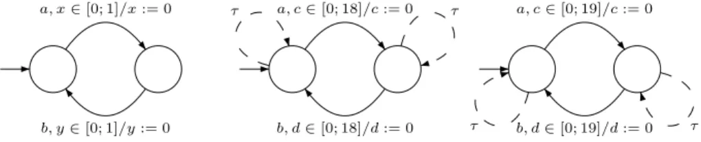
If several clocks are not reset in some transitions, then the entry regions are multi-dimensional, and the volume functions therefore depend on several real variables. Hence, we cannot reduce the integral equation to an ordinary differ-ential equation, which makes it difficult to find the eigenfunction symbolically. Instead, we can use standard iterative procedures for eigenvalue approximation for positive operators. Recall that the volume function satisfies 𝑣𝑛 = 𝛹𝑛1. The
following theorem is close to Thms. 16.1-16.2 from [3].
Theorem 4. If for some 𝛼, 𝛽 ∈ IR, 𝑚 ∈ IN the following inequality holds: 𝛼𝑣𝑚≤
𝑣𝑚+1≤ 𝛽𝑣𝑚, and the volume 𝑉𝑚= 𝑣𝑚(𝑞0, 0) > 0, then log 𝛼 ≤ ℋ ≤ log 𝛽.
Proof. Applying the positive operator 𝛹𝑛 to the inequalities 𝛼𝑣
𝑚 ≤ 𝑣𝑚+1 ≤
𝛽𝑣𝑚, and using the formula 𝑣𝑛= 𝛹𝑛1 we obtain that for all 𝑛
𝛼𝑣𝑚+𝑛 ≤ 𝑣𝑚+𝑛+1≤ 𝛽𝑣𝑚+𝑛.
From this by induction, we prove that for all 𝑛 𝛼𝑛𝑣𝑚≤ 𝑣𝑚+𝑛≤ 𝛽𝑛𝑣𝑚.
1. Transform 𝒜 into the fleshy region-split form.
2. Choose an 𝑚 and compute symbolically the piecewise polynomial func-tions 𝑣𝑚and 𝑣𝑚+1.
3. Check that 𝑣𝑚(𝑞0, 0) > 0.
4. Compute 𝛼 = min(𝑣𝑚+1/𝑣𝑚) and 𝛽 = max(𝑣𝑚+1/𝑣𝑚).
5. Conclude that ℋ ∈ [log 𝛼; log 𝛽].
Table 3.Iterative algorithm: bounding ℋ
𝑚 𝑣𝑚(𝑥) 𝛼 𝛽 log 𝛼 log 𝛽 0 1 0 1 1 1 − 𝑥 0.5 1 -1 0 2 1 − 𝑥 − 1/2 (1 − 𝑥)2 0.5 0.667 -1 -0.584 3 1/2 (1 − 𝑥) − 1/6 (1 − 𝑥)3 0.625 0.667 -0.679 -0.584 4 1/3 (1 − 𝑥) + 1/24 (1 − 𝑥)4 −1/6 (1 − 𝑥)3 0.625 0.641 -0.679 -0.643 5 5 24(1 − 𝑥) + 1 120 (1 − 𝑥) 5 −1/12 (1 − 𝑥)3 0.6354 0.641 -0.6543 -0.643 6 2 15(1 − 𝑥) − 1 720 (1 − 𝑥) 6 + 1 120 (1 − 𝑥) 5 − 1 18 (1 − 𝑥) 3 0.6354 0.6371 -0.6543 -0.6506 7 61 720(1 − 𝑥) − 1 5040 (1 − 𝑥) 7 + 1 240 (1 − 𝑥) 5 − 5 144 (1 − 𝑥) 3 0.6364 0.6371 -0.6518 -0.6506
Table 4.Iterating the operator for 𝒜3(ℋ = log(2/𝜋) ≈ log 0.6366 ≈ −0.6515)
We apply this to the initial state (𝑞0, 0) (remember that 𝑉𝑛= 𝑣𝑛(𝑞0, 0)):
𝛼𝑛𝑉𝑚≤ 𝑉𝑚+𝑛≤ 𝛽𝑛𝑉𝑚.
Take a logarithm, divide by 𝑚 + 𝑛 and take a lim sup𝑛→∞ (remember that
ℋ = lim sup𝑛→∞log 𝑉𝑛/𝑛):
log 𝛼 ≤ ℋ ≤ log 𝛽
(we have used the fact that 𝑉𝑚> 0). ⊓⊔
This theorem yields a procedure8to estimate ℋ summarized in Table 3.
Example: Again 퓐3 We apply the iterative procedure above to our running
example 𝒜3. As explained in Sect. 4.1, we can just consider the operator on
𝐶(0; 1)
𝛹 𝑓 (𝑥) = ∫ 1−𝑥
0
𝑓 (𝑠) 𝑑𝑠. The iteration results are given in Table 4.
8
One possible optimization is to compute 𝛼 and 𝛽 separately on every strongly con-nected reachable component of the automaton, and take the maximal values.
5
Discretization Approach
5.1 Discretizing the Volumes
Another approach, we first published in [13], is to volume/entropy computation is by discretization. This approach sheds also a new light on the information-theoretic interpretation of entropy. The discretizations of timed languages we use are strongly inspired by [14, 15].
5.2 𝜺-words and 𝜺-balls
We start with a couple of preliminary definitions. Take an 𝜀 = 1/𝑁 > 0. A timed word 𝑤 is 𝜀-timed if all the delays in this word are multiples of 𝜀. Any 𝜀-timed word 𝑤 over an alphabet 𝛴 can be written as 𝑤 = ℎ𝜀(𝑣) for an untimed
𝑣 ∈ 𝛴 ∪ {𝜏 }, where the morphism ℎ𝜀is defined as follows:
ℎ𝜀(𝑎) = 𝑎 for 𝑎 ∈ 𝛴, ℎ𝜀(𝜏 ) = 𝜀.
The discrete word 𝑣 with ticks 𝜏 (standing for 𝜀 delays) represents in this way the 𝜀-timed word 𝑤.
Example Let 𝜀 = 1/5, then the timed word 0.6𝑎0.4𝑏𝑎0.2𝑎 is 𝜀-timed. Its repre-sentation is 𝜏 𝜏 𝜏 𝑎𝜏 𝜏 𝑏𝑎𝜏 𝑎.
The notions of 𝜀-timed words and their representation can be ported straight-forwardly to languages.
For a timed word 𝑤 = 𝑡1𝑎1𝑡2𝑎2. . . 𝑡𝑛𝑎𝑛 we introduce its North-East
𝜀-neighbourhood like this: ℬ𝑁 𝐸
𝜀 (𝑤) = {𝑠1𝑎1𝑠2𝑎2. . . 𝑠𝑛𝑎𝑛 ∣ ∀𝑖 (𝑠𝑖∈ [𝑡𝑖; 𝑡𝑖+ 𝜀])} .
For a language 𝐿, we define its NE-neighbourhood elementwise: ℬ𝜀𝑁 𝐸(𝐿) =
∪
𝑤∈𝐿
ℬ𝑁 𝐸𝜀 (𝑤). (17)
The next simple lemma will play a key role in our algorithm (here #𝐿 stands for the cardinality of 𝐿).
Lemma 4. Let 𝐿 be some finite set of timed words of length 𝑛. Then Vol(ℬ𝑁 𝐸𝜀 (𝐿)) ≤ 𝜀𝑛#𝐿.
If, moreover, 𝐿 is 𝜀-timed, then Vol(ℬ𝑁 𝐸
𝜀 (𝐿)) = 𝜀𝑛#𝐿.
Proof. Notice that for a timed word 𝑤 of a length 𝑛 the set ℬ𝑁 𝐸
𝜀 (𝑤) is a
hyper-cube of edge 𝜀 (in the delay space), and of volume 𝜀𝑛. Notice also that
neigh-bourhoods of different 𝜀-timed words are almost disjoint: the interior of their intersections are empty. With these two remarks, the two statements are
5.3 Discretizing Timed Languages and Automata
Suppose now that we have a timed language 𝐿 recognized by a timed automaton 𝒜 satisfying A2-A5 and we want to compute its entropy (or just the volumes 𝑉𝑛). Take an 𝜀 = 1/𝑁 > 0. We will build two 𝜀-timed languages 𝐿− and 𝐿+
that under- and over-approximate 𝐿 in the following sense:
ℬ𝑁 𝐸𝜀 (𝐿−) ⊂ 𝐿 ⊂ ℬ𝜀𝑁 𝐸(𝐿+). (18)
The recipe is like this. Take the timed automaton 𝒜 accepting 𝐿. Discrete automata 𝐴𝜀+ and 𝐴𝜀− can be constructed in two stages. First, we build counter
automata 𝐶𝜀
+ and 𝐶−𝜀. They have the same states as 𝒜, but instead of every
clock 𝑥 they have a counter 𝑐𝑥 (roughly representing 𝑥/𝜀). For every state add
a self-loop labelled by 𝜏 and incrementing all the counters. Replace any reset of 𝑥 by a reset of 𝑐𝑥. Whenever 𝒜 has a guard 𝑥 ∈ [𝑙; 𝑢] (or 𝑥 ∈ (𝑙; 𝑢), or some
other interval), the counter automaton 𝐶𝜀
+ has a guard 𝑐𝑥 ∈ [𝑙/𝜀− 𝐷; 𝑢/𝜀 − 1].
(always the closed interval) instead, where 𝐷 is as in assumption A4. At the same time, 𝐶𝜀
− has a guard 𝑐𝑥 ∈ [𝑙/𝜀; 𝑢/𝜀 − 𝐷]. Automata 𝐶+𝜀 and 𝐶−𝜀 with
bounded counters can be easily transformed into finite-state ones 𝐴𝜀
+ and 𝐴𝜀− .
Lemma 5. Languages 𝐿+= ℎ𝜀(𝐿(𝐴𝜀+)) and 𝐿− = ℎ𝜀(𝐿(𝐴𝜀−)) have the required
property (18). Proof (sketch). Inclusion ℬ𝑁 𝐸
𝜀 (𝐿−) ⊂ 𝐿. Let a discrete word 𝑢 ∈ 𝐿(𝐴𝜀−), let 𝑣 = ℎ𝜀(𝑢) be its
𝜀-timed version, and let 𝑤 ∈ ℬ𝑁 𝐸
𝜀 (𝑣). We have to prove that 𝑤 ∈ 𝐿. Notice
first that 𝐿(𝐴𝜀
−) = 𝐿(𝐶−𝜀) and hence 𝑢 is accepted by 𝐶−𝜀. Mimic the run of
𝐶−𝜀 on 𝑢, but replace every 𝜏 by an 𝜀 duration, thus, a run of 𝒜 on 𝑣 can
be obtained. Moreover, in this run every guard 𝑥 ∈ [𝑙, 𝑢] is respected with a security margin: in fact, a stronger guard 𝑥 ∈ [𝑙, 𝑢−𝐷𝜀] is respected. Now one can mimic the same run of 𝒜 on 𝑤. By definition of the neighbourhood, for any delay 𝑡𝑖 in 𝑢 the corresponding delay 𝑡′𝑖 in 𝑤 belongs to [𝑡𝑖, 𝑡𝑖+ 𝜀]. Clock
values are always sums of several (up to 𝐷) consecutive delays. Whenever a narrow guard 𝑥 ∈ [𝑙, 𝑢 − 𝐷𝜀] is respected on 𝑣, its “normal” version 𝑥′ ∈ [𝑙, 𝑢]
is respected on 𝑤. Hence, the run of 𝒜 on 𝑤 obtained in this way respects
all the guards, and thus 𝒜 accepts 𝑤. We deduce that 𝑤 ∈ 𝐿. ⊓⊔
Inclusion 𝐿 ⊂ ℬ𝑁 𝐸
𝜀 (𝐿+). First, we define an approximation function on IR+as
follows: 𝑡 = ⎧ ⎨ ⎩ 0 if 𝑡 = 0 𝑡 − 𝜀 if 𝑡/𝜀 ∈ IN+ 𝜀⌊𝑡/𝜀⌋ otherwise.
Clearly, 𝑡 is always a multiple of 𝜀 and belongs to [𝑡 − 𝜀, 𝑡) with the only exception that 0 = 0.
Now we can proceed with the proof. Let 𝑤 = 𝑡1𝑎1. . . 𝑡𝑛𝑎𝑛 ∈ 𝐿. We define its
𝜀-timed approximation 𝑣 by approximating all the delays: 𝑣 = 𝑡1𝑎1. . . 𝑡𝑛𝑎𝑛.
By construction 𝑤 ∈ ℬ𝑁 𝐸
𝑥 ∈ [𝑙; 𝑢]. Notice that the clock value of 𝑥 on this run is a sum of several (up to 𝐷) consecutive 𝑡𝑖. If we try to run 𝒜 over the approximating word 𝑣, the
value 𝑥′ of the same clock at the same transition would be a multiple of 𝜀 and
it would belong to [𝑥 − 𝐷𝜀; 𝑥). Hence 𝑥′∈ [𝑙− 𝐷𝜀, 𝑢 − 𝜀]. By definition of 𝐶. +
this means that the word 𝑢 = ℎ−1
𝜀 (𝑣) is accepted by this counter automaton.
Hence 𝑣 ∈ 𝐿+.
Let us summarize: for any 𝑤 ∈ 𝐿, we have constructed 𝑣 ∈ 𝐿+ such that
𝑤 ∈ ℬ𝑁 𝐸
𝜀 (𝑣). This concludes the proof. ⊓⊔
5.4 Counting Discrete Words
Once the automata 𝐴𝜀
+ and 𝐴𝜀− constructed, we can count the number of words
with 𝑛 events and its asymptotic behaviour using the following simple result. Lemma 6. Given an automaton ℬ over an alphabet {𝜏 } ∪ 𝛴, let
𝐿𝑛= 𝐿(ℬ) ∩ (𝜏∗𝛴)𝑛.
Then (1) #𝐿𝑛 is computable; and (2) lim𝑛→∞(log #𝐿𝑛/𝑛) = log 𝜌ℬ with 𝜌ℬ a
computable algebraic real number.
Proof. We proceed in three stages. First, we determinize ℬ and remove all the useless states (unreachable from the initial state). These transformations yield an automaton 𝒟 accepting the same language, and hence having the same car-dinalities #𝐿𝑛. Since the automaton is deterministic, to every word in 𝐿𝑛
cor-responds a unique accepting path with 𝑛 events from 𝛴 and terminating with such an event.
Next, we eliminate the tick transitions 𝜏 . As we are counting paths, we obtain an automaton without silent (𝜏 ) transitions, but with multiplicities representing the number of realizations of every transition. More precisely, the procedure is as follows. Let 𝒟 = (𝑄, {𝜏 } ∪ 𝛴, 𝛿, 𝑞0). We build an automaton with multiplicities
ℰ = (𝑄, {𝑒}, 𝛥, 𝑞0) over one-letter alphabet. For every 𝑝, 𝑞 ∈ 𝑄 the multiplicity
of the transition 𝑝 → 𝑞 in ℰ equals the number of paths from 𝑝 to 𝑞 in 𝒟 over words from 𝜏∗𝛴. A straightforward induction over 𝑛 shows that the number of
paths in 𝒟 with 𝑛 non-tick events equals the number of 𝑛-step paths in ℰ (with multiplicities).
Let 𝑀 be the adjacency matrix with multiplicities of ℰ. It is well known (and easy to see) that the #𝐿(𝑛) (that is the number of 𝑛-paths) can be found as the sum of the first line of the matrix 𝑀𝑛
−. This allows computing #𝐿(𝑛).
Moreover, using Perron-Frobenius theorem we obtain that #𝐿(𝑛) ∼ 𝜌𝑛 where 𝜌
is the spectral radius of 𝑀 , the greatest (in absolute value) real root 𝜆 of the
integer characteristic polynomial det(𝑀 − 𝜆𝐼). ⊓⊔
5.5 From Discretizations to Volumes
As soon as we know how to compute the cardinalities of under- and over- ap-proximating languages #𝐿−(𝑛) and #𝐿+(𝑛) and their growth rates 𝜌−and 𝜌+,
Theorem 5. For a timed automaton 𝒜 satisfying A2-A5, the 𝑛-volumes of its language satisfy the estimates:
#𝐿−(𝑛) ⋅ 𝜀𝑛≤ 𝑉𝑛≤ #𝐿+(𝑛) ⋅ 𝜀𝑛.
Proof. In inclusions (18) take the volumes of the three terms, and use Lemma 4. ⊓ ⊔ Theorem 6. For a timed automaton 𝒜 satisfying A2-A5, the entropy of its language satisfies the estimates:
log(𝜀𝜌−) ≤ ℋ(𝐿(𝒜)) ≤ log(𝜀𝜌+).
Proof. Just use the previous result, take the logarithm, divide by 𝑛 and pass to
the limit. ⊓⊔
We summarize the algorithm in Table 5.
1. Choose an 𝜀 = 1/𝑁 .
2. Build the counter automata 𝐶𝜀
−and 𝐶+𝜀.
3. Transform them into finite automata 𝐴𝜀
−and 𝐴𝜀+.
4. Eliminate 𝜏 transitions introducing multiplicities. 5. Obtain adjacency matrices 𝑀−and 𝑀+.
6. Compute their spectral radii 𝜌−and 𝜌+.
7. Conclude that ℋ ∈ [log 𝜀𝜌−; log 𝜀𝜌+].
Table 5.Discretization algorithm: bounding ℋ
This theorem can be used to estimate the entropy. However, it can also be read in a converse direction: the cardinality of 𝐿 restricted to 𝑛 events and discretized with quantum 𝜀 is close to 2ℋ𝑛/𝜀𝑛. Hence, we can encode ℋ − log 𝜀
bits of information per event. These information-theoretic considerations are made more explicit in Sect. 6 below.
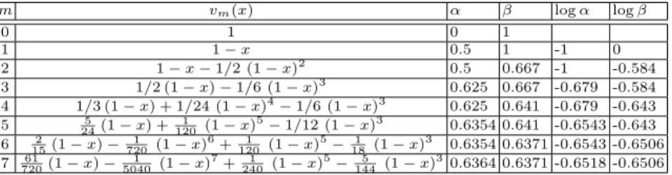
A Case Study. Consider the example 𝐿3= {𝑡1𝑎𝑡2𝑏𝑡3𝑎𝑡4𝑏 ⋅ ⋅ ⋅ ∣ 𝑡𝑖+ 𝑡𝑖+1∈ [0; 1]}
from Sect. 2.2. We need two clocks to recognize this language, and they are never reset together. We choose 𝜀 = 0.05 and build the automata on Fig. 5 according to the recipe (the discrete ones 𝐴+ and 𝐴− are too big to fit on the figure).
We transform 𝐶0.05
− and 𝐶+0.05, into 𝐴+ and 𝐴−, eliminate silent transitions
and unreachable states, and compute spectral radii of adjacency matrices (their sizes are 38x38 and 40x40): #𝐿0.05
− (𝑛) ∼ 12.41𝑛, #𝐿0.05+ (𝑛) ∼ 13.05𝑛. Hence
12.41𝑛⋅ 0.05𝑛≤ 𝑉
𝑛 ≤ 13.05𝑛⋅ 0.05𝑛, and the entropy
𝑎, 𝑥 ∈ [0; 1]/𝑥 := 0 𝑏, 𝑦 ∈ [0; 1]/𝑦 := 0 𝑎, 𝑐 ∈ [0; 18]/𝑐 := 0 𝑏, 𝑑 ∈ [0; 18]/𝑑 := 0 𝜏 𝜏 𝑎, 𝑐 ∈ [0; 19]/𝑐 := 0 𝑏, 𝑑 ∈ [0; 19]/𝑑 := 0 𝜏 𝜏
Fig. 5.A two-clock timed automaton 𝒜3and its approximations 𝐶−0.05and 𝐶+0.05. All 𝜏 -transitions
increment counters 𝑐 and 𝑑.
Taking a smaller 𝜀 = 0.01 provides a better estimate for the entropy: ℋ ∈ [log 0.6334; log 0.63981] ⊂ (−0.659; −0.644).
We proved in 4.1 that the true value of the entropy is ℋ = log(2/𝜋) ≈ log 0.6366 ≈ −0.6515.
6
Kolmogorov Complexity of Timed Words
To interpret the results above in terms of information content of timed words we state, using similar techniques, some estimates of Kolmogorov complexity of timed words. Recall first the basic definition from [16] (see also [17]). Given a partial computable function (decoding method) 𝑓 : {0; 1}∗× 𝐵 → 𝐴, a
descrip-tion of an element 𝑥 ∈ 𝐴 knowing 𝑦 ∈ 𝐵 is a word 𝑤 such that 𝑓 (𝑤, 𝑦) = 𝑥. The Kolmogorov complexity of 𝑥 knowing 𝑦, denoted 𝐾𝑓(𝑥∣𝑦) is the length of the
shortest description. According to Kolmogorov-Solomonoff theorem, there exists the best (universal) decoding method providing shorter descriptions (up to an additive constant) than any other method. The complexity 𝐾(𝑥∣𝑦) with respect to this universal method represents the quantity of information in 𝑥 knowing 𝑦. Coming back to timed words and languages, remark that a timed word within a “simple” timed language can involve rational delays of a very high complexity, or even uncomputable real delays. For this reason, we consider timed words with finite precision 𝜀. For a timed word 𝑤 and 𝜀 = 1/𝑁 we say that a timed word 𝑣 is a rational 𝜀-approximation of 𝑤 if all delays in 𝑣 are rational and 𝑤 ∈ ℬ𝑁 𝐸
𝜀 (𝑣)9.
Theorem 7. Let 𝒜 be a timed automaton satisfying A2-A4, 𝐿 its language, ℋ its entropy. For any rational 𝛼, 𝜀 > 0, and any 𝑛 ∈ IN large enough there exists a timed word 𝑤 ∈ 𝐿 of length 𝑛 such that the Kolmogorov complexity of all the rational 𝜀-approximations 𝑣 of the word 𝑤 is lower bounded as follows
𝐾(𝑣∣𝑛, 𝜀) ≥ 𝑛(ℋ + log 1/𝜀 − 𝛼). (19)
Proof. By definition of the entropy, for 𝑛 large enough 𝑉𝑛> 2𝑛(ℋ−𝛼).
9
In this section, we use such South-West approximations 𝑣 for technical simplicity only.
Consider the set 𝑆 of all timed words 𝑣 violating the lower bound (19) 𝑆 = {𝑣 ∣ 𝐾(𝑣∣𝑛, 𝜀) ≤ 𝑛(ℋ + log(1/𝜀) − 𝛼)} .
The cardinality of 𝑆 can be bounded as follows:
#𝑆 ≤ 2𝑛(ℋ+log(1/𝜀)−𝛼)= 2𝑛(ℋ−𝛼)/𝜀𝑛. Applying Lemma 4 we obtain
Vol(ℬ𝑁 𝐸
𝜀 (𝑆)) ≤ 𝜀𝑛#𝑆 ≤ 2𝑛(ℋ−𝛼)< 𝑉𝑛.
We deduce that the set 𝐿𝑛of timed words from 𝐿 of length 𝑛 cannot be included
into ℬ𝑁 𝐸
𝜀 (𝑆). Thus, there exists a word 𝑤 ∈ 𝐿𝑛∖ ℬ𝑁 𝐸𝜀 (𝑆). By construction, it
cannot be approximated by any low-complexity word with precision 𝜀. ⊓⊔ Theorem 8. Let 𝒜 be a timed automaton satisfying A2-A4, 𝐿 its language, 𝛼 > 0 a rational number. Consider a “bloated” automaton 𝒜′, which is like 𝒜, but
in all the guards each constraint 𝑥 ∈ [𝑙, 𝑢] is replaced by 𝑥 ∈ [𝑙−𝛼, 𝑢+𝛼]. Let ℋ. ′be
the entropy of its language. Then the following holds for any 𝜀 = 1/𝑁 ∈ (0; 𝛼/𝐷), and any 𝑛 large enough.
For any timed word 𝑤 ∈ 𝐿 of length 𝑛, there exists its 𝜀-approximation 𝑣 with Kolmogorov complexity upper bounded as follows:
𝐾(𝑣∣𝑛, 𝜀) ≤ 𝑛(ℋ′+ log 1/𝜀 + 𝛼).
Proof. Denote the language of 𝒜′ by 𝐿′, the set of words of length 𝑛 in this
language by 𝐿′
𝑛 and its 𝑛-volume by 𝑉𝑛′. We remark that for 𝑛 large enough
𝑉′
𝑛< 2𝑛(ℋ
′+𝛼/2)
.
Let now 𝑤 = 𝑡1𝑎1. . . 𝑡𝑛𝑎𝑛 in 𝐿𝑛. We construct its rational 𝜀-approximation as
in Lemma 5: 𝑣 = 𝑡1𝑎1. . . 𝑡𝑛𝑎𝑛. To find an upper bound for the complexity of 𝑣
we notice that 𝑣 ∈ 𝑈 , where 𝑈 is the set of all 𝜀-timed words 𝑢 of 𝑛 letters such that ℬ𝑁 𝐸
𝜀 (𝑢) ⊂ 𝐿′𝑛. Applying Lemma 4 to the set 𝑈 we obtain the bound
#𝑈 ≤ 𝑉𝑛′/𝜀𝑛< 2𝑛(ℋ
′+𝛼/2)
/𝜀𝑛.
Hence, in order to encode 𝑣 (knowing 𝑛 and 𝜀) it suffices to give its number in a lexicographical order of 𝑈 , and
𝐾(𝑣∣𝑛, 𝜀) ≤ log #𝑈 + 𝑐 ≤ 𝑛(ℋ′+ log 1/𝜀 + 𝛼/2) + 𝑐 ≤ 𝑛(ℋ′+ log 1/𝜀 + 𝛼)
for 𝑛 large enough. ⊓⊔
Two theorems above provide close upper and lower bounds for complexity of 𝜀-approximations of elements of a timed language.
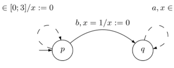
However, the following example shows that because we removed Assumption A5, in some cases these bounds do not match and ℋ′ can possibly not converge
𝑝 𝑞 𝑏, 𝑥 = 1/𝑥 := 0
𝑎, 𝑥 ∈ [0; 5]/𝑥 := 0 𝑎, 𝑥 ∈ [0; 3]/𝑥 := 0
Fig. 6.A pathological automaton
Example 1. Consider the automaton of Fig. 6. For this example, the state 𝑞 does not contribute to the volume, and ℋ = log 3. Nevertheless, when we bloat the guards, both states become “usable” and, for the bloated automaton ℋ′ ≈
log 5. As for Kolmogorov complexity, for 𝜀-approximations of words from the sublanguage 1𝑏([0; 5]𝑎)∗it behaves as 𝑛(log 5+log(1/𝜀)). Thus, for this bothering
example, the complexity matches ℋ′ rather than ℋ.
7
Conclusions and Further Work
In this paper, we have defined size characteristics of timed languages: volume and entropy. The entropy has been characterized as logarithm of the leading eigenvalue of a positive operator on the space of continuous functions on a part of the state space. Three procedures have been suggested to compute it.
Research in this direction is very recent, and many questions need to be studied. We are planning to explore practical feasibility of the procedures de-scribed here and compare them to each other. We believe that, as usual for timed automata, they should be transposed from regions to zones. We will explore po-tential applications mentioned in the introduction.
Many theoretical questions still require exploration. It would be interesting to estimate the gap between our upper and lower bounds for the entropy (we believe that this gap tends to 0 for strongly connected automata) and establish entropy computability. We would be happy to remove some of Assumptions A1-A5, in particular non-Zenoness. Kolmogorov complexity estimates can be improved, in particular, as shows Example 1, it could be more suitable to use another variant of entropy, perhaps ℋ+= max ℋ
𝑞, where the entropy is maximized with respect
to initial states 𝑞. Extending results to probabilistic timed automata is another option. Our entropy represents the amount of information per timed event. It would be interesting to find the amount of information per time unit. Another research direction is to associate a dynamical system (a subshift) to a timed language and to explore entropy of this dynamical system.
Acknowledgment
The authors are thankful to Oded Maler for motivating discussions and valuable comments on the manuscript.
References
1. Ben Salah, R., Bozga, M., Maler, O.: On timed components and their abstraction. In: SAVCBS’07, ACM (2007) 63–71
2. Lind, D., Marcus, B.: An introduction to symbolic dynamics and coding. Cam-bridge University Press (1995)
3. Krasnosel’skij, M., Lifshits, E., Sobolev, A.: Positive Linear Systems: The method of positive operators. Number 5 in Sigma Series in Applied Mathematics. Helder-mann Verlag, Berlin (1989)
4. Bucci, G., Piovosi, R., Sassoli, L., Vicario, E.: Introducing probability within state class analysis of dense-time-dependent systems. In: QEST’05, IEEE Computer Society (2005) 13–22
5. Sassoli, L., Vicario, E.: Close form derivation of state-density functions over dbm domains in the analysis of non-Markovian models. In: QEST’07, IEEE Computer Society (2007) 59–68
6. Bertrand, N., Bouyer, P., Brihaye, T., Markey, N.: Quantitative model-checking of one-clock timed automata under probabilistic semantics. In: QEST’08, IEEE Computer Society (2008) 55–64
7. Asarin, E., Pokrovskii, A.: Use of the Kolmogorov complexity in analyzing control system dynamics. Automation and Remote Control (1) (1986) 25–33
8. Rojas, C.: Computability and information in models of randomness and chaos. Mathematical Structures in Computer Science 18(2) (2008) 291–307
9. Brudno, A.: Entropy and the complexity of the trajectories of a dynamical system. Trans. Moscow Math. Soc. 44 (1983) 127–151
10. Asarin, E., Caspi, P., Maler, O.: Timed regular expressions. Journal of the ACM 49(2002) 172–206
11. Alur, R., Dill, D.L.: A theory of timed automata. Theoretical Computer Science 126(1994) 183–235
12. Asarin, E., Degorre, A.: Volume and entropy of regular timed languages: Analytic approach. To appear in proceedings of FORMATS’09 (2009)
13. Asarin, E., Degorre, A.: Volume and entropy of regular timed languages: Dis-cretization approach. To appear in proceedings of Concur’09 (2009)
14. Asarin, E., Maler, O., Pnueli, A.: On discretization of delays in timed automata and digital circuits. In: CONCUR’98. LNCS 1466, Springer-Verlag (1998) 470–484 15. Henzinger, T.A., Manna, Z., Pnueli, A.: What good are digital clocks? In:
ICALP’92. LNCS 623, Springer-Verlag (1992) 545–558
16. Kolmogorov, A.: Three approaches to the quantitative definition of information. Problems of Information Transmission 1(1) (1965) 1–7
17. Li, M., Vit´anyi, P.: An introduction to Kolmogorov complexity and its applications. 3 edn. Springer (2008)