A numerical model for calculating temperature profiles in ice covers

Publisher’s version / Version de l'éditeur:

Vous avez des questions? Nous pouvons vous aider. Pour communiquer directement avec un auteur, consultez la

première page de la revue dans laquelle son article a été publié afin de trouver ses coordonnées. Si vous n’arrivez pas à les repérer, communiquez avec nous à PublicationsArchive-ArchivesPublications@nrc-cnrc.gc.ca.

Questions? Contact the NRC Publications Archive team at

PublicationsArchive-ArchivesPublications@nrc-cnrc.gc.ca. If you wish to email the authors directly, please see the first page of the publication for their contact information.

https://publications-cnrc.canada.ca/fra/droits

L’accès à ce site Web et l’utilisation de son contenu sont assujettis aux conditions présentées dans le site LISEZ CES CONDITIONS ATTENTIVEMENT AVANT D’UTILISER CE SITE WEB.

Technical Memorandum (National Research Council of Canada. Division of Building Research); no. DBR-TM-114, 1974

READ THESE TERMS AND CONDITIONS CAREFULLY BEFORE USING THIS WEBSITE.

https://nrc-publications.canada.ca/eng/copyright

NRC Publications Archive Record / Notice des Archives des publications du CNRC :

https://nrc-publications.canada.ca/eng/view/object/?id=d282a642-2338-445c-a9a2-a042f442bdbe https://publications-cnrc.canada.ca/fra/voir/objet/?id=d282a642-2338-445c-a9a2-a042f442bdbe This publication could be one of several versions: author’s original, accepted manuscript or the publisher’s version. / La version de cette publication peut être l’une des suivantes : la version prépublication de l’auteur, la version acceptée du manuscrit ou la version de l’éditeur.

Access and use of this website and the material on it are subject to the Terms and Conditions set forth at

A numerical model for calculating temperature profiles in ice covers

Goodrich, L. E.

PREFACE

The thermal regime of river ice has long been of importance for hydro-electric operation, flooding, navigation

and water supply problems. In recent years i t has become

increasingly important for such diverse problems as determining the effect of warm water discharge from nuclear plants on

downstream ice conditions, the effect of river ice on fish spawning grounds, and the effect of snow disposal in rivers

on water quality and ice formation. In recognition of this

increasing importance, the Snow and Ice Subcommittee of the Associate Committee on Geotechnical Research sponsored a research seminar on the subject, 24-25 October 1974, at

Foret Montmorency Research Station of Laval University. This

Technical Memorandum records the papers presented at this

seminar. There was much informal discussion during the seminar

but only written discussion has been included in the Proceedings. Several of the papers are presented in summary form; additional information can be obtained by writing to the authors.

The seminar was divided into three sessions; the first dealt with surface heat exchange, the second with ice formation in rivers, and the third with operational problems. The seminar was designed to be informal, with attendance

limited to those active in one or more of the session topics. The seminar was fortunate in having active participation from several guests from the united States.

The Associate Committee wishes to express its appreciation to Dr. Bernard Michel for handling the local arrangements so effectively, to Dr. Andre LaFond, Dean of the Faculty of Forestry and Geodesy, for giving the welcoming

address and for making the excellent facilities at the Research Station available for the seminar, and to Mr. G.P. Williams, Chairman of the Working Group, responsible for organizing the seminar.

Carl B. Crawford, Chairman,

Associate Committee on Geotechnical Research.

PREFACE

Le regime thermique de la glace de riviere tient depuis longtemps de l'importance dans les problemes de

fonctionnement hydro-electrique, de debordement de cours

d'eau, de navigation et d'approvisionnement d'eau. Ces

dernieres annees, il prend de plus en plus d'importance au regard de divers problemes tels que celui de determiner l'effet d'un deversement d'eau chaude provenant d'une

installation nucleaire sur les conditions de la glace en aval, l'effet de la glace de riviere sur les frayeres, et l'effet de l'action de disposer de la neige dans les rivieres sur la

qualite de l'eau et la formation de la glace. Reconnaissant

cette importance toujours grandissante, Ie Sous-comite de la glace et de la neige du Comite associe de recherches

geotechniquesa commandite un debat sur Ie sujet, les 24 et 25

octobre 1974,

a

Montmorency de l'Dniversite Laval. Le present memoire

technique rapporte les articles qui ont ete presentes lors de

cette etude. Bien que la seance ait comporte beaucoup de

discussion sans formalites, Ie proces-verbal ne comprend que

la discussion ecrite. Plusieurs articles ont ete presentes

sous forme de resumes; des renseignements supplementaires sont disponibles en ecrivant aux auteurs.

Le debat comportait trois seances, dont la

premlere traitait de transmission de la chaleur

a

la deuxieme, de la formation de la glace de riviere; et la

troisieme, de problemes de fonctionnement. II avait ete

prevu que Ie debat serait sans formalites, l'assistance etant limitee aux personnes qui s'occupent d'un theme ou plus des

seances. Le debat recevait avec plaisir la participation

active de plusieurs invites des Etats-Unis.

Le Comite-associe desire exprimer son appreciation

! Monsieur Bernard Michel qui slest occupe si efficacement

de faire les preparatifs necessaires,

!

Doyen de la Faculte de foresterie et de geodesie, qui a lu l'adresse et a rendu disponible les excellentes commodites

de la Station de recherche, et

a

President du Groupe de travail, qui est responsable de l'organisation du debat.

Le President,

Comite associe de recherches geotechniques

TABLE OF CONTENTS - TABLE DES MATIERES FIRST SESSION - PREMIERE SEANCE

Chairman Le President

B. Pratte,

National Research Council of Canada

1. Heat Transfer from

Open-Water Surfaces in Winter.

2. Radiation and Evaporation

Heat Loss during Ice Fog Conditions.

3. Energy Transfer in Snow.

4. A Numerical Model for

Calculating Temperature Profiles in an Ice Cover.

5. Convective Heat Transfer

at an Ice-Water Inter-face.

SECOND SESSION - DEUXIEME SEANCE

N. Marcotte, Universite de Moncton. T. McFadden, U.S. Army CRREL, Alaska. D.M. Gray and D.H. Male, University of Saskatchewan. L.E. Goodrich, National Research Council of Canada.

J.E. Cowley and S.T. Lavender, Acres Consulting Services Ltd. 2 18 28 44 60 Chairman Le President G.P. Williams,

National Research Council of Canada

Introductory Remarks - G.P. Williams 78

1. A Preliminary

Investiga-tion and Experimental Set-up for the Study of Frazil Formation in Water with Surface Waves.

2. Mechanisms of Ice Growth

at the Ice-Water-Air Interface in a Laboratory Tank. G. Tsang, Canada Centre for Inland Waters. B. Michel and T. OlD. Hanley, Universite Laval. 82 96

3.

4.

5.

Supercooling and Frazil Ice Formation in a Small Sub-arctic Stream.

Ice Regime Investigations on the Moira River at Belleville, Ontario. Ecological Implications of Frazil and Anchor Ice in High Mountain Streams. T. Osterkamp, University of Alaska. K.W. Lathem, Crysler and Lathem Ltd. C.B. Stalnaker and J.L. Arnette, Utah State University. 104 109 121

THIRD SESSION - TROISIEME SEANCE Chairman Le President D. Foulds, Environment Canada 1. Practical Application of Probability Forecasts of Water Surface Temperatures of St. Lawrence River -Kingston to Montreal.

2. Winter Temperature

Measurements in Lakes along the Churchill River River Diversion Route.

3. Statistical Analysis of

Niagara Ice Boom Effects on Water Temperature.

4. Regime Thermique des

Grands Reservoirs Soumis aux Conditions de Glace.

5. Ice Jams Related to

Climatological and Hydraulic Parameters

-Yukon River at Dawson City.

6. Alaska River Thermal

Problems, Research and Design Criteria.

Summary - ｒ･ｳｵｭｾ

Registration List - Liste

J. Robinson and D. Witherspoon, Environment Canada. V.C. Kartha, Manitoba Hydro. C.H. Atkinson, Acres Consulting Services Ltd. R. Lariviere et F. Fonseca, Hydro-Ouebec. H.R. Kivisild and J. Penel, FENCO. R.F. Carlson, University of Alaska. B. Michel 128 134 145 152 170 177 181 184

NATIONAL RESEARCH COUNCIL OF CANADA Ser TA701 N28t2 no.114 SLOG. RFS National

HEAT TRANSFER FROM OPEN-WATER SURFACES IN WINTER N. Marcotte

INTRODUCTION

Heat-transfer from open-water areas in rivers or

reservoirs in winter is considered. Water temperature is

assumed to be DoC.

A brief review at the heat budget method will be given together with comments on various expressions for

caluclating each term of the budget. A comparison will then

be made between the overall K coefficient in mid-winter at Montreal and Nitchequon.

A) HEAT BUDGET

The sum of heat losses and gains by solar radiation, long wave radiation, evaporation and convection per unit area and per unit time is written:

a

where s

units: cal/cm2-day.

(a) Long wave radiation:

Q = (- c a T4 ) + (f' e ' aT4 ) RI e a water emissivity

=

=

=

1

:a]

(After Anderson, Raphael, Ref. 4)

e_a vapor pressure in the air, mb

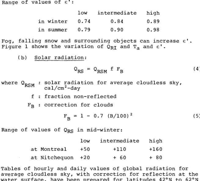
Range of values of £': in winter in summer low 0.74 0.79 intermediate 0.84 0.90 high 0.89 0.98

Fog, falling snow and surrounding objects can increase £'.

Figure 1 shows the variation of QRI and Ta and

£'.

(b) Solar radiation:

(4 )

where QRSM solar radiation for average cloudless sky,

cal/cm2-day

fraction non-reflected correction for clouds

F

=

B (5)

Range of values of QRS in mid-winter:

low intermediate high

at Montreal +50 +110 +160

at Nitchequon +20 + 60 + 80

Tables of hourly and daily values of global radiation for average cloudless sky, with correction for reflection at the water surface, have been prepared for latitudes 42°N to 62°N

(Ref. 3).

(c) Turbulent exchange:

Bulk aerodynamic formulae are used: Q_C

=

Replacing constants by their numerical value with appropriate units we obtain: Q C

=

=

where CH,C_E Pa V T_e T a e_a e_s q c_pa

=

=

bulk transfer coefficients

air density, g/cm3

wind velocity, km/hr, with V._mln = 3 km/hr

water temperature, °c air temperature, °c

vapor pressure in the air, mb

saturation pressure at water temperature, mb vapor concentration, gig

0.2397 cal/gOC (at 0° C)

597.3 cal/g (at O°C)

with CH

=

which permits calculation of QC when QE is known and conversely.

Equations (6) and (7) indicate that both QC and QE

are functions of ｾ Pa and CH. The wind velocity V is dependent

on height, atmospheric stability and geometry of surface

(Ref. 1,2), and in certain cases it will be necessary to apply

a correction factor to the value of V measured at the weather

station. Air density Pa varies with air temperature as shown

in figure 2. _{Finally the coefficient CH is strongly dependent}

on atmospheric stability (Ref. 1,2).

where C

HN coefficient in neutral stability

C_{HN =} 1 3_• X 10-3

(9 )

(10)

Fs multiplying factor

During summer typical values of Fs are in the order

of 0.8 to 1.2. In mid-winter strong instability over an

open-water surface results in a much larger Fs which is in the

order of 1.0 to 2.5. Figure 3 shows two expressions of Fs in

function of the Richardson number. With floating ice and

increased surface roughness, CH is expected to be still higher. As a consequence "summer formulae" of evaporation need correction for Pa and CH when used in winter -- if

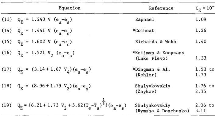
Table 1 gives the calculated value of CE for a few

evaporation formulae using Pa at 20aC.

TABLE 1. EVAPORATION FORMULAE

Equation Reference C x 10-3 E (13) Q_E 1. 243 V (e -e ) Raphael 1.09 a s (14) Q_E 1.441 V (e -e ) *Co1heat 1. 26 a s

(15) Q_E 1.602 V (e -e ) Richards &Webb 1. 40 a s

(16) Q_E 1.521 V

2 (e -e )a s *Keijrnan &Kooprnans

(Lake Flevo) 1.33 (17) Q_E

=

4)(ea-e )s *Dingman &A1. 1. 53 to

(Kohler) 1.73

(18) Q_E

=

2)(ea-e )s Shu1yakovskiy_(Zaykov) 1. 76 to_2.35

.l-(19) Q

E

=

Figure 4 shows a comparison of QC calculated from

equations (13), (17), (19) and (6) with (11) and (12) when

V

=

of Ta and V based on equation (19), (Ref. 5).

(d) Sum of components: See figure 7.

B) AVERAGE K COEFFICIENT

The overall transfer coefficient K is expressed:

Q

=

e a (20)

The units of K are cal/cm2 day aC. Knowing the numerical

value of the overall coefficient, a rough estimate of Q can

be made. Here the variation of K with meteorological

param-eters is examined.

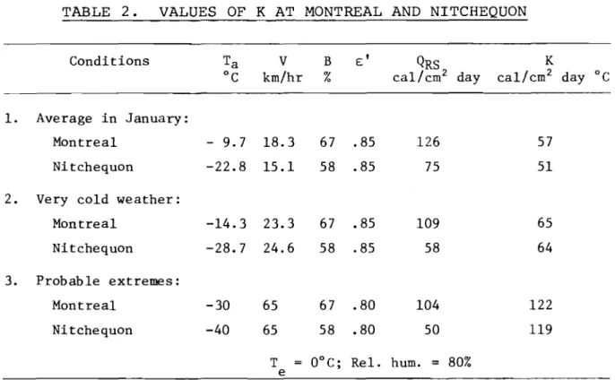
Figure 8 indicates the variation of K with Ta and

V, while Table 2 gives representative values of K at Montreal

and Nitchequon. The turbulent exchange terms have been

cal-culated from equation (19); use of other expressions in

Table 1 results in" smaller values of K.

TABLE 2. VALUES OF K AT MONTREAL AND NITCHEQUON

Conditions 1. Average in January: Montreal Nitchequon V km/hr - 9.7 18.3 -22.8 15.1 B % 67 .85 58 .85 126 75 K cal/cm2 _{day °c} 57 51 2. Very cold weather:

Montreal Nitchequon 3. Probable extremes: -14.3 -28.7 23.3 24.6 67 58 .85 .85 109 58 65 64 Montreal Nitchequon -30 -40 65 65 67 .80 58 .80 104 50 122 119 T O°C; ReI. hum.

=

e

Since K is strongly dependent on V, an attempt has

been made to find another overall coefficient that would be more nearly constant:

Q

=

e a (21)

Figure 9 indicates that J _{changes little with Ta,}

but varies sensibly with V, thus reflecting the influence of

Fs.

CONCLUSION

Heat transfer from open-water surfaces in winter can

be calculated with a maximum error of probably less than ± 40%.

The turbulent exchange terms are of major importance and their determination is uncertain at high atmospheric instabilities, particularly at low wind velocities.

REFERENCES

1. Haugen, D.A. 1973. "Workshop on Micrometeorology."

American Meteorological Society.

2. Krauss, E.B. 1972. "Atmosphere-Ocean Interaction."

Oxford University Press.

3. Marcotte, N. and V.L. Duong. 1974. "Rayonnement solaire

global et rayonnement solaire absorbe par l'eau, ciel

clair moyen, latitude 400N

a

Departement de Genie, Universite de Moncton.

4. Raphael, J.M. 1962. "Prediction of Temperature in Rivers

and Reservoirs." Proceedings of the A.S.C.E., J. Power Div., July 1962, 157-181.

5. Shulyakovskiy, L.G. 1969. "Formula for computing

Evaporation with Allowance for the Temperature of the

Free Water Surface." Soviet Hydrology; Selected Papers,

0 ro o 0 ｾ

o

...

-

-

-

£-

-

o

=

(After Businger, ref. 1 )

_ _ _ _ _ Fs

=

o

ｾＡ o! 'tJ I C\l ! E

I-··,··J

01

: '

i

"0

ｲＮｴｧｾｪｦｬＨｊＬＬ｜

_I"

_{］ｾｏＬｩ}

I

-10 -20 -30

Tair, °C

I I' ,.. I 1 :_{ｲＭｾＺＭｾＺＧＭ} ｾＢ "--I ' , ' , , i I i i IDj" h ,\cl',tm.l Q '"40

Fig.

"1

fOR

ｌ

...

ｾＮｌＺ

i

<.

p.e

<b.•

.ｾ･ｌ ..

-tuua.

ad.

4

_9.•

a

ｄｯｾ･ｨｾｈＧｫｯ

-00 I ' ,I

ｉｾｾ｛

;

Fig.,l:-t--J ;:

e1'a.V)

.r .

+--1

'1

DISCUSSION N. Marcotte

Three authors at this Seminar in speaking of the subject of heat exchange from open-water surface used three

different systems of units. The following conversion factors

for Q and K are useful for

comparison:-1 cal/cm2/day

=

1 cal/cm2/day/oC

=

=

The overall transfer coefficient for ice-fog is

then:-For the St. Lawrence river* at freeze-up the conversion

is:-Thermal budget computations for the St. Lawrence river with average meteorological conditions at Montreal in

November and water temperatures measured in 1972 (Figure 1,

Robinson and Witherspoon) appear to indicate that

Rimsha-Donchenko equations give too high values of K while

these obtained from the Kohler equation are in better agreement

with observations. (These equations are given in Reference 5

of this summary and in Dingman and AI, Research Report 206, U.S. ARMY CRREL, Hanover, N.H.)

RADIATION AND EVAPORATION HEAT LOSS DURING ICE FOG CONDITIONS T. McFadden

EVAPORATION

Evaporation accounts for a major portion of the heat dissipated from an open water surface during winter months. It is also recognized as a large contributor to the ice fog in

the Fairbanks, Alaska, area. A knowledge of the "order of

magnitude" of this heat loss is essential to ice fog suppression. Evaporation is a function of many interacting

variables. Water temperature and surface conditions influence

the vapour flux leaving the surface: while wind, air temperature,

and relative humidity influence the flux of vapour returning to

the water. The interaction of these variables has made

mathe-matical predictions of evaporation difficult.

One of the most important parameters in winter is

induced air movement. During ice fog conditions a unique

situation is developed. The air near the ground (below 50

meters) is nearly quiescent, so that conventional wind

measure-ments show zero velocity. The air over the warm open water

surface of a cooling pond is far from still, however. The

temperature differences between air and water can be greater

than 50°C. Air near the water surface is warmed and rises

over the pond, forming a characteristic plume. Therefore,

although meteorological measurements in the vicinity of a cooling pond may show zero wind, convective air currents are usually present and they greatly influence evaporation.

Although the extremely cold air can hold very little moisture, the continued flow of new air into the pond area to replace the air that rises vertically in the convection plume provides a mass transfer mechanism that can carry off large

amounts of vapour. Therefore, it might be expected that

empirical equations developed for warmer windier climates may underpredict the evaporation during times when meteorological measurements indicate wind to be absent.

Evaporation Equations

Most empirically derived equations have used the same basic form as Dalton's Law (1802):

E= (f(u)) (e -e .)

where E

₌

ai

=

₌

w

temperature of the water surface f(u)

₌

where "a" and "b" are empirically derived constants and "u" is the average wind speed.

Several authors have proposed empirical equations for predicting evaporation based on data from a variety of situations the following formulae are among several of these that were compared to data gathered from a power plant cooling pond at Eielson Air Force Base, Alaska.

Author Kohler

Rimsha and Donchenko Behlke and McDougall

Formula Q E

=

=

=

Where QE is the evaporative heat loss, Tw is water temperature (OC), Ta is air temperature (OC), and "u" is wind speed (m/s).

Using computer fitting techniques, the following revised equations were developed which more closely correlate with the measured results when ice fog conditions were

approached: Author

Revised Rimsha and Donchenko equation:

Revised Formula

Q_E

=

w a w a (4 )

Revised Dalton Eq.: Q

E

=

The effect of wind during winter conditions in interior Alaska was found to be minimal and, during ice fog conditions, wind was found to be negligible both in the studies at Eielson and as reported by Behlke and McDougall (1973). The effect of wind would have been significant if i t had existed, but the very condition of ice fog is one that comes about only in the absence of wind. Therefore, wind showed no effect in analysis of the measured data.

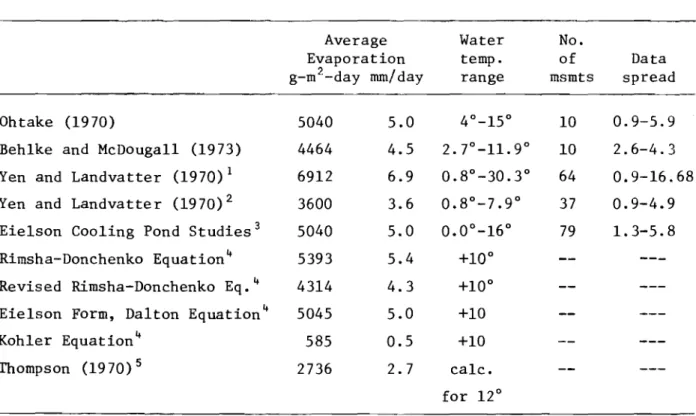
Evaporation Measurement During Ice Fog

A few investigators have measured the evaporation rates prevailing during ice fog conditions. The following table summarizes the reported results and comparisons to the above equations:

EVAPORATION RATES DURING ICE FOG TEMPERATURES Average Evaporation g-m2-day rom/day Water temp. range No. of msmts Data spread Ohtake (1970) 5040 5.0 4°_15° 10 0.9-5.9

Behlke and McDougall (1973) 4464 4.5 2.7°-11.9° 10 2.6-4.3 Yen and Landvatter (1970)1 6912 6.9 0.8°-30.3° 64 0.9-16.68

Yen and Landvatter (1970)2 3600 3.6 0.8°-7.9° 37 0.9-4.9

Eie1son Cooling Pond Studies 3 5040 5.0 0.0°-16° 79 1. 3-5. 8 Rimsha-Donchenko Equationq 5393 5.4 +10°

Revised Rimsha-Donchenko Eq. q 4314 4.3 +10° Eie1son Form, Dalton Equationq 5045 5.0 +10

Kohler Equationq 585 0.5 +10

Thompson (1970)5 2736 2.7 calc.

for 12° lLaboratory measurements, all values included.

20 n l y values for air temperatures below freezing included.

3Values for the Eielson cooling pond were the average values for all conditions during the testing throughout the winter. qValues were calculated for -20°C air temperature and +lO°C

water temperature.

5u sing Thornwaite and Holzman's equation (reported by Ohtake, 1970) •

Fig. 1 compares the various equations above. RADIATION

The net radiation loss during ice fog from an open water area such as a power plant cooling pond is dependent on several variables. The emission from the water surface is dependent on the temperature and emissivity. The emissivity of a surface has been established by several investigators, and the value of 0.97 is well agreed upon (Raphael, 1962).

Calculation of the radiation leaving the surface, therefore, is a relatively easy task.

Radiation incoming to the pond can be divided into

two distinct categories: short-wave radiation from the sun;

and long-wave radiation from the atmosphere, surrounding

geographic features, or man-made structures. The incoming

solar radiation during ice fog conditions is a negligible

portion of the radiation heat balance of an open water surface

during ice fog (McFadden 1974). The problem of estimating

the net radiation loss during ice fog conditions, therefore, is reduced to that of estimating the effective back radiation from the atmosphere and subtracting it from the outgoing

radiation. A number of investigators have proposed empirical

equations to estimate the value of atmospheric back radiation

as a function of the vapour pressure at the surface. Several

of these equations were compared to radiation measurements

taken during winter conditions generally and ice fog conditions in particular at the Eielson Air Force Base cooling pond.

Computer fitting techniques were used to evaluate optimum

constants for the equations and a standard error was calculated (Figure 2).

Atmospheric Radiation Equations

Equation Constants as Presented by Original Author

b d Percent a c _{Std error} Brunt's Eq. .60 .042 27.0 Angstrom's ｅｱｾ .806 .236 .115 24.3 Elsasser's Eq. .21 .22 73.8 Anderson's Eq. .74 .025 .0049 .00054 18.5

Constants Resulting from Eielson Data

Brunt's ｅｱｾ .807 .029 13.7

Angstrom's Eq. .658 .201 .375 14.6

Elsasser's ｅｱｾ .848 .039 14.1

Anderson's Eq. .814 .11 .0054 .00059 10.7

Although the differences in standard error are not great, i t is interesting to note that the equations originally proposed by the various authors generally exhibited consider-ably greater standard error than did the equations resulting

accuracy may be obtained when calculating atmospheric radiation during ice fog conditions and perhaps general winter conditions by the use of the equations correlated to these data.

The final form of each equation is:

Revised Brunt's Eq. Q = (.807+ .0291e"") oT4

a a

Revised Angstrom's Eq. Q = (.658 - .201 exp (-.375e )) oT4

a a

Revised Elsasser's Eq. Q =(.848+.039 log e ) OT4

a a

(6 )

(7)

(8 )

Revised Anderson's Eq. Q

a

=

(.0054 - .000594Nexp (-.06h))] 0'1,4 (9)

Ice fog plays a significant role in attenuating the

radiative heat losses from an open water surface. This effect

is more pronounced as the temperature falls, due to increased back radiation from the fog layer, until the maximum fog density

is reached. Atmospheric back radiation then declines as air

temperatures continue to fall.

Wind was found to exhibit a significant effect on

the net measured radiation. This was probably because wind

removed the relatively warm "vapour blanket" over the pond. This ice fog "blanket" contributed much greater atmospheric

back radiation than did the normal clear arctic sky. Therefore,

long-wave radiation losses were greater during windy periods. In interior Alaska wind is not present in sufficient velocity during ice fog periods to cause a measurable effect; however, along the north and west coast of Alaska, wind is often present when air temperatures plunge sufficiently to cause ice fog. Long-wave radiation losses during these times would probably exceed those during ice fog.

Using Bowen's ratio to estimate the heat loss by convection allows a heat balance of the surface to be made. The following table shows the major components of the heat loss at the surface both during ice fog conditions and when meteorologic conditions approach those conducive to the

Temp. * Diff 10 20 30 40

Heat Balances at the Surface

Q_E Q_H Q_R Q_T % % % w/m2 25.5 25.5 49 157 25 38 37 319 25.5 43 32 490 24 47 29 643

*Water surface temperature of 10°C is assumed. CONCLUSIONS

Evaporation comprises on the order of one-fourth of total heat loss from a cooling pond surface during winter

conditions. Radiation losses are slightly higher than

evaporation, but do not amount to more than one-third of the

total except at low water-air temperature differences.

Con-vective losses make up the balance, and are the predominate means of heat loss during ice fog conditions.

This suggests that the cooling pond's contribution of ice fog to the total problem may be much less than

previously believed. Radiation losses attenuate as ice fog

thickens, but always remain a significant portion of the

total. This is probably due to the relative shallowness of

the ice fog blanket and the fact that only a small fraction of the long-wave "back" radiation emitted by the ice fog is directed toward the pond.

REFERENCES

Behlke, C. and J. McDougall, 1973. Polyethylene Sheeting as

a Water surface Cover in Sub-zero Temperatures. Proceedings

of the 24th Alaska Science Conference, University of Alaska, Fairbanks, Alaska.

Benson, C.S., 1970. Ice Fog. United States Army Cold

Regions Research and Engineering Laboratory, Research Report 121, Hanover, N.H.

Bowen, I.S., 1926. The ratio of Heat Losses by Conduction and

Evaporation from any Water Surface. physical Review Series #2

Vol. 27, pp. 779-787.

Dingman, S.W., W.F. Weeks, and Y.C. Yen, 1967. The effects of

Thermal Pollution on River Ice Conditions. U.S. Army Cold

Regions Research and Engineering Laboratory Research Report #206, Hanover, N.H.

McFadden, T., 1974. Ice Fog Suppression from Power Plant

Cooling Ponds. U.S. Army Cold Regions Research and Engineering

Laboratory (in publication), Hanover, N.H.

Raphael, I., 1962. Prediction of Temperature in Rivers and

Reservoirs. Proceedings of the American Society of Civil

Engineers, Journal of the Power Division No. P02, Paper 3200, pp. 157-181.

Rimsha, V.A. and R.V. Donchenko, 1958. Winter Heat Losses

from an Open Surface of Water. Trudy Gosudarslvennogo

Gedrologicheskago Institutt Gedrometeoizdat, Leningrad (in Russian).

Yen, Y.C. and G. Landvatte, 1970. Evaporation of Water into

a Sub-zero Air Stream. Water Resources Research, Vol. 6,

[] ｾ

a

:e

W

W

_I

v

L1

Z

_Z

r

0

₀

0

.J

_lSJ

W

r

V

W

_LJW

I

m

v

r

_W

Z

Z

M

W

Il:

_r

0

W

0

lr

u

>

l!l

-

Z

_El

I-

W

w

o:w

r3

P1

_W

I

W

r3

[

_lL

v

w

_Q

J

U.

_C

z

Z

_IT:

_lr

lr1

[j

-

0

1:

W

PJ

W 0

Z

_Z

I

_J

u

J:

₀

n

1-Z

W

IIlN

U.

"

-

hi

I

0

[r

- 8

_n:w

:{

-

J

L1

i-l-

i-

n:

-

v

[

[

W

_I

lr

rr

:t

W

-0

W

v

a.

[1-

_ra

[

r

m

.

L1

>lflWl!l

-

-w

W>l-h.

,f'1

B

ls1

N

N

-

-

lJ1

<

W

>

5501 183H d8A3

/ \ / \ /\

m r-

_m

13 13

lD

_fJ

LJ

W

W

_{L1 V}

v v

v

Ul

U1

W

BBLJI3

LJLJvLJ

II

...

0

V

I

ZLBII

:t

J

Z

D

W W

...

W

mil

ill

1

v

l-

rr

l! ...

wmZ!L

m

LJ

[[

_W

o

a a

n

v

W

I.L

II: lIm

ZZlL-I

LJ

Z

LJ

I

IL

II

l!l

-NPlJ"

P1

W

l

ZO

0

II.

-Oil.

0

-

W

I-W

Ir

v

v.

_II

LJ

n:V

J

19

,

N

:J

...

-

-

l-

II

o

[

₁₁

rI

[l!l

_Jr

1:

W

LJ

n

IrZ

W

...

fl

1:

n.

-LJ

1I

...

1-[(

r

w

W

J

n

LJ

m

f--

It

ZO>r-

3

19

B

B

t3

_B

:r

f'I

W.

SSOl

U1

...

Z

W

t-

W

Z

a

fJ

v

0

L1

n.

W

0:

r

V

t-O

Z

I

z

V

W

Cl

...

u:

J

"

U1

W

w

U1

I.L

_z

v

0

I.L

Ll

Jl!J

-

0:

0

0

n

W

IJ.

1-11.

l

-[[

_W

_v

₀

ww

n:

₁₅₁

_u

IV

:J

-

a

II

-

1-

I

fl1

J

...

W

[

_n.

Vl!l

u

L

It

hi

[Z

W

...

D.

lr.-

₁₁

M

II

1:

rL[L

_L

W

-

...

hi

:J:JlJlWl'lr

- It

UlC>t-L.3

,

B

is

13

s

19

19

i9

B

l::J

l'3

₁₉

-

m

m

r-

u

lJ1

r

PI

1'1

ssm

ENERGY TRANSFER IN SNOW D.M. Gray and D.H. Male INTRODUCTION

During the past several years the Division of Hydrology, University of Saskatchewan, has carried out an extensive field program in Snow Hydrology. One group of studies in this program has been directed to investigation of the energy regime of the snowpack during both "non-melt" and "melt" events. Consideration has also been given to the spatial and temporal variations of some of the energy terms and the transposability of data collected at a point to areal conditions. The data base established includes measurements taken from manually-obtained samples of natural snow, a snow lysimeter installed in the field which is capable of auto-matically monitoring most of the energy terms at short time

intervals as programmed by a HP 2ll4B digital computer and measurements taken from the air.

It is recognized that the presence of a snow layer on an ice surface influences the thermal regime and energy transfer processes of the ice-water matrix thereby affecting such factors as; the rate of growth of ice, its strength properties and its decay or disappearance. In this abstract the energy terms important to the thermal regime of a snow-pack are discussed.

THE ENERGY EQUATION

Consider the energy equation for a snowpack in the following form:

(1)

dU

where dt = the rate of internal energy change per unit area (watts/sq. meter/hr),

=

interface,

the flux of latent heat at the snow-air interface (evaporation, condensation),

the flux associated with melt water leaving the bottom of the snowpack, and

=

In any experimental study of the energy exchange for a snowpack i t is important that each of these terms be measured independently so that an estimate can be made of the accumulated error inherent in the measuring procedures.

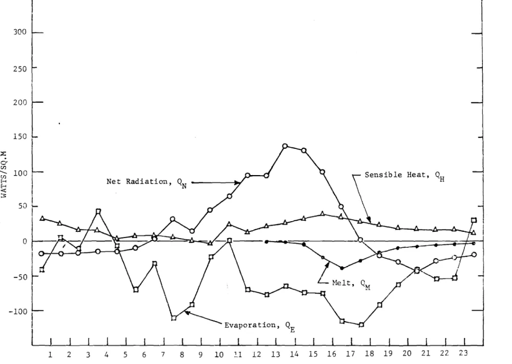
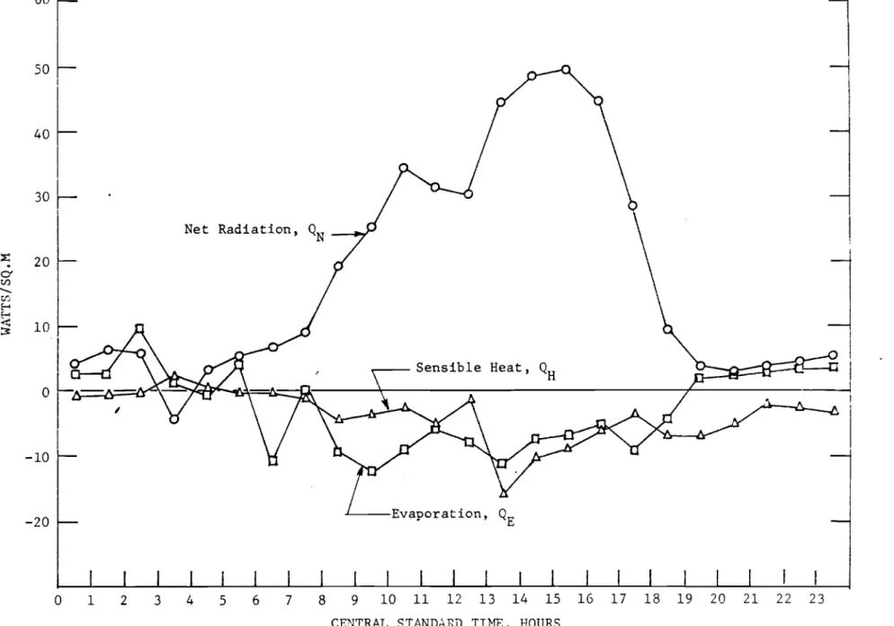
Figures 1 and 2 are typical plots of the terms in Equation (1) over a 24-hour period in the Spring of 1974 when melt

first occurred. On this day the snow depth was approximately

30 cm. Figures 3 and 4 are similar curves for a day in which

no melt water was produced. RADIATIVE TERMS

The term QN of Equation (1) represents the net

all-wave radiation flux to or from the snowpack. Its magnitude

is affected by the short wave radiation incident to the surface, the albedo of the surface and the net long wave

radiation exchange. On the prairies i t has been found that

this flux is extremely important and dominates the thermal regime of the pack during non-melt periods and also the melt phenomenon during the period when snow cover is complete. During the latter part of the melt sequence when the snow

cover is patchy sensible heat becomes a dominant factor. The

important parameters affecting this term are discussed below. Albedo

Albedo, A, is the ratio of the reflected, QRS' to

incident, QIS, short wave radiation. It depends on atmospheric

and surface conditions and the properties of the snow. Manz

(1974) reported the absorptivity of a snowpack is greatly

affected by the presence of foreign matter content (material

other than ice, water or air) primarily because of the effects of such material on the extinction coefficients and albedos.

Similarly, his findings indicated that the albedo characteristics of a snowpack decrease rapidly with an increase in density and particle size.

Figure 5 shows the temporal decay curves of spatial

albedo (within the wave length band 0.2 ｾｭ to 1.2 ｾｭＩ measured

during 1974 over a lake surface and open fields in Saskatchewan. The curves show three distinct characteristics:

(1 )

( 2)

High albedos during the non-melt periods; 70 to 75 percent.

A rapid decay of the albedos of both surfaces during

the melt period. Melt on the land surfaces started

( 3) A close association between the albedos of the two

surfaces. Major differences between the two curves

occurs only during the melt period. The more rapid

decrease in the lake albedo is likely caused by ponded surface runoff and the shallower depth of

snow cover on the lake surface. Water began ponding

on the lake surface on April 18th. By April 24th

the land was mostly free of snow and water covered

the ice on the lake surface. The result accentuates

the importance of snow cover in governing the albedo of a surface.

Other theoretical and experimental studies conducted have indicated that:

(1 )

(2)

Flux

The underlying boundary surface only exerts measure-able influence on the surface albedo when the depth

of snow is very shallow Ｈｾ 2 - 4 cm).

The water content of snow exerts little influence on its optical qualities providing if it is not turbid and does not cause extensive modifications of the snow structure.

The flux of monochromatic diffuse radiation at any depth within a snowpack is characterized by the extinction

coefficient, absorptivity and the speed of light. All these

parameters are mathematically related. The extinction

coefficient and albedo are highly wavelength dependent. The

extinction coefficient exhibits a general increase at

wave-lengths greater than the near-infrared (> 0.7 ｾｭＩ whereas

the albedo decreases in this wavelength interval. O'Neill

and Gray (1973) and Manz (1974) have shown that the

broad-band radiation flux profile can be defined by the simple exponential function.

F

₌

0

where F

₌

F

₌

0

b

₌

Figure 6 (taken from Manz (1974)) shows the measured

flux profiles for three wavelength intervals; 0.42 ｾｭ

<

A

<

0.72 ｾｭ

<

A

<

<

A

<

natural snow sample (density

=

coefficients for the three intervals were 0.42 ｣ｭｾｬＬ 0.455 cm-1

From the data given in the figure it may be noted; (1)

( 2)

( 3)

All flux profiles follow reasonably closely the

exponential function (Equation 2).

A larger percentage of the incident flux of the smaller wavelengths penetrates to a greater depth

than radiation of larger wavelengths. The extinction

coefficient of the shorter wavelength band is less than the coefficient for the larger wavelength band. For all cases, less than 50 percent of the incident flux passes below 1 cm and less than 10 percent

penetrates below 4 cm. Note: the wavelength

interval; 0.42 ｾｭ

<

<

approxi-mately 61 percent of the short wave radiation (optical

air mass

=

SENSIBLE HEAT FLUX (QH)

The magnitude of this term is strongly influenced by the local wind velocity and the temperature gradient above

the snow surface. It is not uncommon for sensible heat to

reach 50 percent of the maximum net radiation on a given day

even with wind speeds below 0.5 m/sec. In evaluating this

term i t is necessary to measure the wind and temperature

profiles above the snow surface. Meaningful measurements of

these profiles are not possible unless the local terrain is relatively flat and free from obstructions such as trees and

buildings. This restriction makes i t extremely difficult to

estimate sensible heat flux in many natural situations. One

instrument has been developed which is designed to measure this term directly (Bailey, Mitchell and Beckman, 1973) but i t has yet to be evaluated under cold weather conditions. EVAPORATION AND CONDENSATION (QE)

The magnitude of this term is governed by the vapour pressure gradient above the snow surface as well as the wind

velocity gradients. During days in which melt does not occur

the net amount of evaporation over a 24-hour period is

generally negligible (see Figure 3). Although significant

evaporation can occur around solar noon this flux is usually counteracted by equally significant condensation in the early

evening. As melt progresses a small net evaporation can be

measured (0.1 mm/day) and once the pack reaches a depth of

less than 5 cm evaporation rates of 0.3 mm/hr have been

measured. Figure 1 shows a day in which evaporation was at

MELT WATER (QM)

This term can be measured with reasonable accuracy

using a properly designed snow lysimeter. On the prairies

i t is significant only during the last 3 or 4 days of the

melt period. A great many investigations of melt water

through snow have been undertaken. Recently Colbeck (1974)

has developed a reasonably simple analysis of the movement of melt water through a snowpack on the assumption that the

gravity force has a major influence on water movement for an

isothermal snowpack. He shows a good comparison of the

results of this analysis with measurements. GROUND HEAT FLUX (QG)

This term has a range of from 0 - 3 watts/m2 _{at the}

Bad Lake Watershed and is generally insignificant in energy

balance considerations. Because of its small magnitude this

flux is not included in Figures 1 and 3 although i t is included

in the summation term of Figures 2 and 4. If an energy balance

is conducted over a period of several days the cumulative effect of this flux may become important since i t does not normally change direction over a 24-hour period.

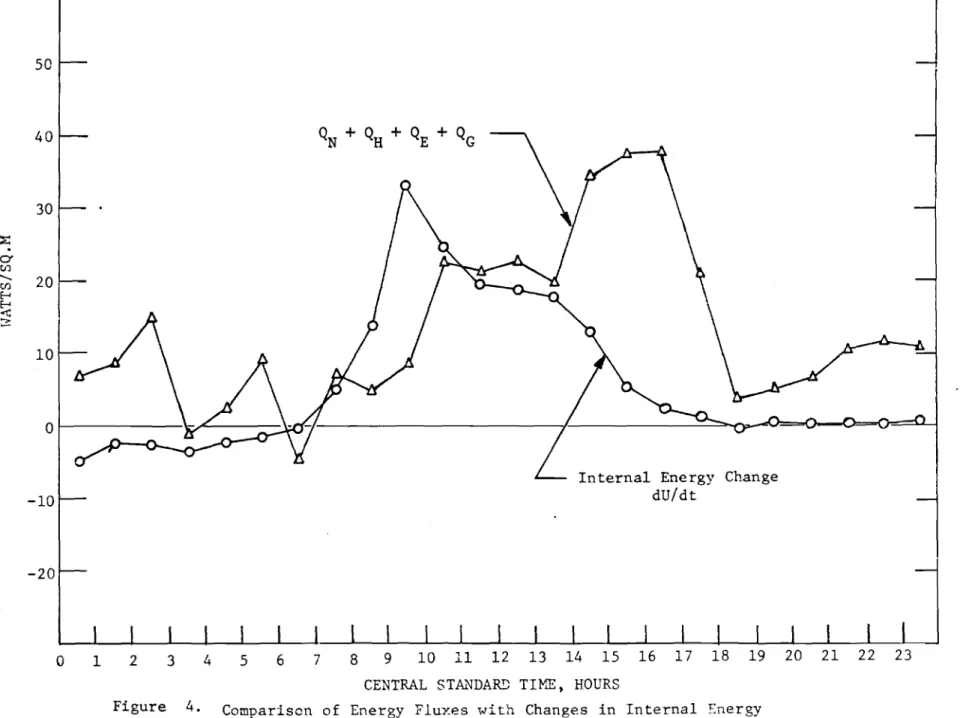
INTERNAL ENERGY OF THE SNOWPACK (dU/dt)

For snowpacks having a depth of 50 cm or less this term is a significant factor in the overall energy budget

during the melt period (Figure 2) but is of less significance

when melt does not occur (Figure 4). The internal energy

consists of a component for the solid, liquid and vapour phases of the snow and has the form;

(3 )

In the above expression

)!, _{the snow depth,}

p

=

C

₌

v

T_m

₌

The subscript 1 refers to ice, )!, to liquid water and v to

vapour.

During non-melt days the liquid density is zero and the evaluation of internal energy involves a measurement of snow depth, mean temperature and snow density; all of which

MIDDLE BOTTOM

(- 6 cm) (- 13 cm)

.885 .59

.917 .968

water is present in the pack p£ must be measured and this we

have found extremely difficult to do with a high degree of accuracy hence the large difference between the curves in

Figures 2 and 4. This term causes a great deal of trouble

when attempts are made to model the snow melt process. In

the early part of the melt season, runoff is commonly produced in the afternoon but the pack cools at night and

freezes. A significant amount of energy is required the next

day to bring the pack to the point where melt water is again

produced. This freeze-thaw process has proven extremely

difficult to model. In particular it is difficult to predict

the time at which melt water will first appear on any given

day. An attempt is currently being made to develop a model

for the Prairies which will overcome this problem.

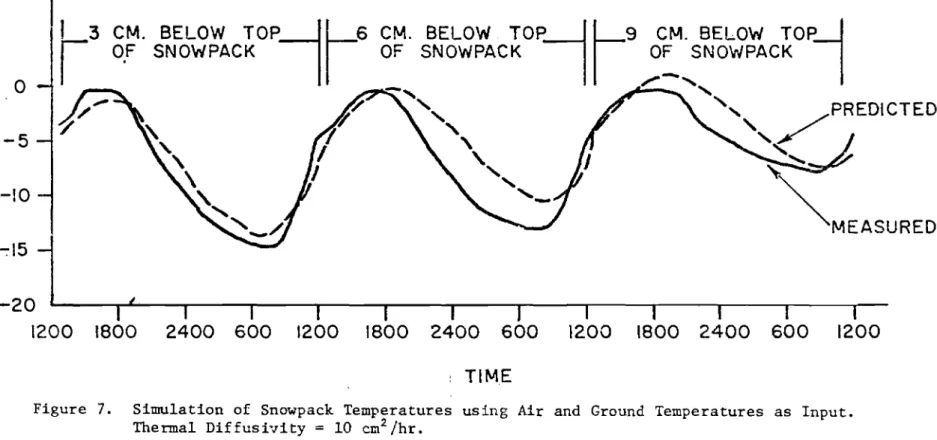
Dybvig (1974) found that the temperature regime

within a snowpack during "non-melt" periods and hence internal energy changes could be predicted using a simple conduction model based on solution of the unsteady state energy diffusion

equation. Figure 7 shows a typical set of results obtained

with the model which demonstrate that the predicted and

measured temperatures are in close agreement. Dybvig tested

the sensitivity of the model to different inputs; namely, net radiation and ground heat flux and air and ground temperatures. His findings indicated little improvement in the predictability of the model from using flux values over that obtained using

temperature data. Table 1 gives the correlation matrix between

air, ground and snow temperatures.

TABLE 1

TEMPERATURES IN THE SNOWPACK TOP

(- 1 cm)

Air Temperature .987

Ground Temperature .629

Air Temperature taken at 20 cm - above ground Ground Temperature taken at 4.8 cm - below ground

These correlation coefficients indicate that the variation in the air and ground temperatures explain 97.4 percent and 93.7 percent of the possible variation in the temperatures at the

top and bottom of the pack. This model is currently being

extended to the melt period by incorporating the analysis developed by Colbeck (1974).

REFERENCES

Bailey, R.T., J.W. Mitchell, and W.A. Beckman, 1973. "An

Experimental Method for Determining Convective Heat Transfer

from a Desert Surface." ASME Paper No. 73-WA/HT-9. Presented

at the Winter Annual Meeting ASME. November, 1973.

Colbeck, S.C., 1974. "On Predicting Water Runoff from a Snow

Cover." Paper 1.6, Advanced Concepts and Techniques in the

Study of Snow and Ice Resources. National Academy of Sciences,

Washington, D.C., 1974.

Dybvig, W., 1973. "Prediction of Snow Temperature Regimes

Using a Heat Conduction Model." Research Report No. 14,

Division of Hydrology, College of Engineering, University of Saskatchewan, Saskatoon.

Manz, D.H., 1974. "Interaction of Solar Radiation with Snow."

Unpublished M.Sc. Thesis, University of Saskatchewan, Saskatoon. O'Neill, A.D.J., and Don M.

Penetration through Snow." Symposium, The Role of Snow 1:227-242.

Gray, 1973. "Solar Radiation

Proc. of Unesco-WMO-IASH

300 250 200

ｾ

l

ｾ

ｾ

o

o

I

J

z

-50 r

ｾ

Internal Energy Change dr/dt

1

l

I

l

ｾ

ｉｾ

ｌｾ

I

-

CENTRAL ｓｔＦｾｄａｒｏ TIME, HOURS

Figure "-..,

.

so

r---

ｾ

I

I

ｾ

I

J

.

-

<

I

I

O r - -

-1

l(

I

o

ｃｅｎｔｒｐｾ STANDARD TIME, HOURS

50

]

Internal Energy Change dU/dt Q_N+ Q_H+ Q_E+ Q_G 0' ｾｾ ....ＯｾＭＭＭ 40 -10 30 ::.::

.

-

/\

}

/

ｾ

\

ａｾｉ

I

o

CENTRAL STAJ.'lDAR2; TIME, HOURS

Figure 4. Comparison of Energy Fluxes with Changes in Internal Energy March 31, 1974, Bad Lake Watershed

o

o

ｾ

4°1

. - - - -

60

-a

_•

I

•

I

25

17

27

16

26

FEB. MARCH APRIL

DATE, FEB. THRU APRIL, 1974

3 o» ｾ L> W L> <I 1..1-0:: => o» ｾ 7 0 et:: u... w

a

ｾ CM. BELOW TOP

I 19

l

,.,-

-,

,

,

,

,

_,

'

_"

"'-

ＧＭｾｾＭｾ

II

ｔｏｐｾｾＶ

I

II

ｾ

r

7

I

ｾＱＵ

1

I {

I

I

I

I

I

I

I

I

I

I

w

0

.-

_-5

Figure 7. Simulation of Snowpack Temperatures using Air and Ground Temperatures as Input. Thermal Diffusivity

=

DISCUSSION

B. Goodison

You are involved in detailed measurements during periods of continuously cold weather, and the absolute energy

fluxes may be very small. Would you care to comment on the

measurement errors involved during these cold weather periods? Secondly, would the error of extrapolating these "point" measurements over a local basin be within your measurement errors or is it too unreliable to use these

values over a larger area? If the latter is true, what other

factors (other than adjustment of solar radiation for slope

and aspect) must be considered? D. Male

The measurement errors for the individual terms in the energy budget vary, depending on the climatic conditions. Normally we expect that the difference between the summation of the fluxes and the internal energy will be less than 20% of the flux summation during non-melt periods ON AN HOURLY

BASIS. On days when the wind velocity is light this error

is greater due to the difficulty of evaluating the sensible

heat flux during this condition. For short time periods

during melt errors of 50% or greater are not uncommon because it is extremely difficult to obtain a measure of the internal

energy term. As the time scale is increased these errors are

likely less due to the random variation of the individual terms.

The question of extrapolating point measurements

over a local basin is a major concern of our group. There

are many factors which prevent this at the present time, but the major ones are:

(1)

(2 )

( 3)

Correction of both long and short wave radiation fluxes for slope and aspect.

variation in snow depth. The "effective melt area"

of a watershed is hard to determine. Melt produced

from shallow snowpacks may be released directly whereas melt produced at the top of deeper packs refreezes before reaching the ground.

We have very little idea of how the sensible heat

term is INFLUENCED by local topography. Additionally,

the entire problem of evaluating the components of the energy budget on a spatial basis, particularly under patchy snow cover conditions, has yet to be solved.

Although we feel that we may be able to obtain a fairly close estimate of the total radiative energy to a fairly large area we do not know how this flux is partitioned.

A NUMERICAL MODEL FOR CALCULATING TEMPERATURE PROFILES IN AN ICE COVER

L.E. Goodrich

INTRODUCTION

For problems such as that of estimating ice

pressures due to thermal expansion as well as in the wider context of ice thermal regime studies, temperature variations

within floating ice covers need to be calculated. Because of

the complexities, analytic methods are of limited use. The

flexibility of numerical methods along with their ability to handle a considerably greater degree of physical detail, makes their use highly desirable, if not essential, for theoretical

analyses of the thermal regime of floating ice covers. This

paper describes an efficient and accurate numerical technique for treating the non-linear heat balance boundary conditions that arise in these problems.

Heat transfer calculations for floating ice sheets involve complexities which, while not entirely precluding their use, render analytic techniques cumbersome and of

limited application. For theoretical investigations of the

thermal regime in floating ice covers, the much greater

flexibility of numerical methods, along with their ability to handle a considerably greater degree of physical detail,

renders their use highly desirable, if not essential.

Heat transfer within a floating ice cover may be described by where pc

ｾｾ

=

[k

ｾｾｊ

=

=

=

=

x,t are space, time

(1)

and A(x,t) represents the internal heating rate per unit

volume due to the absorption of penetrating solar radiation.

At the upper boundary surface heat is exchanged with the atmosphere through thermal radiation as well as by

con-vective processes. Although these processes depend on

atmospheric temperature and humidity gradients as well as other factors, such as wind speed and cloud conditions, for calculation purposes i t is usual to represent them by

simplified empirical relations. In the absence of melting,

the heat balance boundary condition at the upper surface may be written as

aT

- k ｾｘｯ

=

o alr 0 0 alr 0 (2 )

where T

air = air temperature at screen height

T = surface temperature

0

a = Stefan-Boltzman constant

H = convective heat transfer coefficient

E = emissivity of ice surface

0

E = effective emissivity factor for the atmosphere

For short-term calculations of temperature changes in ice covers of sufficient thickness, accretion at the ice-water interface will be negligible and the lower boundary condition can be taken as

T (X ,t)

=

e

=

max (3 )

where X_max

=

A variety of numerical schemes is available for

treating the non-linear system constituted by equations (1),

(2) and (3). Although linearization of equation (2) is

probably acceptable for long-term calculations where, in any case, the interest generally centres on ice growth rates, air and surface temperatures may differ considerably during the

course of a day. For diurnal calculations it is preferable

to work with the fully non-linear form of equation (2).

Explicit finite difference formulations of equation (1) with equation (2) are easily written but involve a

stability criterion which severely limits the magnitude of

time step possible. In an attempt to improve accuracy and

reduce the stability restriction, formulations have been written which involve the iterative solution of a single

non-linear algebraic equation corresponding to the surface mode coupled with explicit equations at the interior nodes.

Untersteiner (1971), in a thermodynamic model for sea ice, eliminate the stability restriction by using the Saul'yev

explicit equations. This technique requires short time steps

in order to achieve good numerical accuracy.

Much higher accuracy can be achieved with no

stability restrictions by using implicit formulations. In

general, implicit techniques for non-linear problems require nodal iteration in which the temperature at each node point is successively re-evaluated until a suitable convergence is

achieved. Several iteration cycles are required at each time

step and computation times are relatively high. In addition,

if the number of nodes is large, double precision arithmetic may be necessary in order to reduce cumulative round-off errors.

For problems, such as the one under consideration, where the non-linearity is confined to a single node, it is possible to avoid nodal iteration altogether and it is one of the purposes of this paper to describe such a technique.

The backward difference equations corresponding to

equations (1) and (2) are, for the surface node i

=

+Am+l + COND (Tm+l _ Tm+l)

0 0 1 0

and for interior nodes

where ｔｾ

₌

₌

1 1 1 6x.

₌

-

₌

₌

₌

₌

=

pc

=

( 4)

A

and T means absolute temperature.

Using backward Gaussian elimination with forward substitution (the reverse of the usual process)

8.

=

1max

8._{1 1 1}

=

=

_ Tm+l

E. - .

1max 1max (given)

m m+l

E._{1 1 1}

=

+ COND_{i(1-8 i+ l)):} 1

=

8₁. Tm+ l_1-. 1 + E₁. 1

=

The unknown

ｔｾＫｬ

ｾ｡ｮ

There results the simple quartic equation

(9 )

which can be solved for Tm+ l by any convenient iterative

method. For this type ofOequation the Newton-Ruphson formula

(10)

where zn is the nth estimate of the root, provides rapid

convergence. At each time step, having evaluated the Gaussian

elimination coefficients from equations (6) and (7), equation (9) is solved, after which equation (8) may be used to deter-mine the temperatures at all interior nodes.

This solution technique is efficient and accurate

and not subject to stability restrictions. The method may

also be applied to Crank-Nicholson finite difference as well as finite element formulations.

Monochromatic radiation extinction in clear ice follows the Bouguer-Lambert exponential law

-ax R(x)

=

o (11)

where R

=

=

o

a

=

The absorption coefficient for ice is strongly wavelength dependent. Dividing the solar spectrum (.3-3 ｾｭＩ into N intervals and using values of spectral absorption coeffi-cients an compiled from the literature (Goodrich (1970» along with spectral weights W_{n for the solar radiation}

reaching the earth's surface (Table 1) the total net solar radiation flux at depth in clear ice may be approximated as

R(x)

N _{-a x}

=

n=l

(12)

The normalized heating function 1 dR

=

is shown in Figure 1. It is evident that solar heating in clear ice cannot be represented by a simple exponential law, particularly in the first 30 cm or so.

For more realistic conditions, the ice will contain air inclusions, grain boundaries, cracks and other inhomo-geneities from which the penetrating radiation will be scattered, greatly increasing the effective "extinction" coefficient. A similar situation exists for snow. No

universally accepted theory exists for either case although a simple exponential decay law is considered by many to be appropriate for snow. According to Dunkle and Gier (1953), for snow

R(x)

=

o r

where ｾ

=

la'

=

=

r

=

The coefficients vary widely with density, grain size and

type and other factors. Measurements which, in any case,

generally cover only limited ranges of the visible spectrum,

show little agreement. The literature contains estimates of

ｾ ranging from ｾ .04 cm- 1 _{to 0.16 cm-}1

for ostensibly similar

snow (density 0.42 cm-3

) and the same wavelength ("blue light").

The accompanying figures (2, 3 and 4) illustrate some typical

results calculated using the model described above. For all

three cases radiation heating in clear ice was treated

following equation (12) which yields, for the heating source term in equations (4) and (5).

ａｾＫｬ = Rm+l L: W e-an(x. - DX_{i _ l ) -} L: W e-an(x. + D

2Xi )

1 0 n 1 2 n 1

where

ｒｾＫｬ

Several preliminary runs were made comparing model

results vs an analytic solution for a simplified case. As is

to be expected in view of the extremely strong depth dependence of the solar radiation heating in the upper levels of the ice cover, some care is required in selecting an appropriate grid

spacing. A constant value of 2 cm with time step 0.01 days

was found to give surface temperatures (numerically) accurate

to ｾ l/lO°C and was used in subsequent calculations.

The following parameters were used in all cases:

p

=

c

=

k = 2.2 W/m-K

H

=

of ｾ 7 m/sec)

EO

=

E

=

at ｾ -20°C)

e =

thickness 0.5 metres.

The daily air temperature was assumed to vary

sinusoidally with amplitude 3K about a mean of -20°C, with

maximum temperature at 15:00 hours. Incoming solar radiation

was assumed to follow a sine curve with maximum flux 500 W/m2

at 12:00 hours, with sunrise and sundown at 8:00 and 16:00

hours corresponding to typical midwinter conditions.

Cal-culations were carried through a sufficient number of daily cycles to yield essentially periodic steady state solutions.