HAL Id: hal-02949396
https://hal.archives-ouvertes.fr/hal-02949396
Preprint submitted on 25 Sep 2020HAL is a multi-disciplinary open access
archive for the deposit and dissemination of sci-entific research documents, whether they are pub-lished or not. The documents may come from teaching and research institutions in France or abroad, or from public or private research centers.
L’archive ouverte pluridisciplinaire HAL, est destinée au dépôt et à la diffusion de documents scientifiques de niveau recherche, publiés ou non, émanant des établissements d’enseignement et de recherche français ou étrangers, des laboratoires publics ou privés.
Description of the IMACLIM-Country model: A
country-scale computable general equilibrium model to
assess macroeconomic impacts of climate policies
Gaëlle Le Treut
To cite this version:
Gaëlle Le Treut. Description of the IMACLIM-Country model: A country-scale computable general equilibrium model to assess macroeconomic impacts of climate policies. 2020. �hal-02949396�
Gaëlle Le Treut
CIRED Working Paper
N° 2020-85 - Septembre 2020
Description of the
IMACLIM-Country model
A country-scale computable general
equilibrium model to assess
macroeco-nomic impacts of climate policies
Corresponding author: letreut@centre-cired.fr
Centre international de recherche sur l’environnement et le développement
Model documentation version 1.0
Referring to modeling platform hosted on Github: Le Treut et al. (2019)
Imaclim-Country modeling team :
Current members: Frédéric Ghersi, Gaëlle Le Treut, Julien Lefèvre, Antoine Teixeira, Jean- Charles Hourcade Former member: Emmanuel Combet
Contents
1 Imaclim-Country notations 3
1.1 Variables ofImaclim-Country . . . 3
1.2 Parameters calibrated on statistical data . . . 5
1.3 Exogenous parameters . . . 7
2 Formulary of Imaclim-Country 8 2.1 General equation framework . . . 8
2.2 Growth engine . . . 8
2.3 Producer and Consumer Prices . . . 9
2.4 Households . . . 11
2.4.1 Income formation, savings and investment decision . . . 12
2.4.2 Consumption . . . 13
2.5 Production (institutional sector of firms) . . . 14
2.5.1 Gross disposable income and investment decision . . . 14
2.5.2 Production trade-o↵s . . . 14
2.5.3 Gross operating surplus . . . 16
2.6 Public administrations . . . 16
2.6.1 Tax, social security contributions and fiscal policy . . . 16
2.6.2 Gross disposable income, public spending, investment and transfers . . . 17
2.7 "Rest of the World" . . . 18
2.7.1 Balance of Trade . . . 18
2.7.2 Capital flows and self-financing capacity . . . 19
2.8.1 Goods markets . . . 20
2.8.2 Investment and capital flows . . . 20
2.8.3 Employment . . . 21
2.9 Carbon tax policies . . . 22
3 The accounting framework 23
1
Imaclim-Country notations
Calibration consists in providing a set of values to all variables and then determining the values that should be given to the parameters so that the set of equations defining the model holds. The exercise is therefore to determine what values the parameters must take in order for the values drawn from national accounts to be linked by the set of equations. However, all parameters do not receive their values from the calibration: the carbon tax, for instance, is a purely exogenous parameter; other parameters have their values set according to some econometric estimation on data superseding the national accounts as described by the input-output table and the economic account table. As a result of these distinctions, the notations below are presented in three categories, (i) the variables of the model properly speaking, (ii) the parameters of the model that are calibrated on statistical data, and (iii) the exogenous parameters. Within each of these categories the notation are listed in alphabetical order (the Greek letters are classified according to their English name rather than according to their equivalent in the Latin alphabet).
1.1 Variables ofImaclim-Country
Variable Name Description
↵ij Technical coefficient, quantity of good i entering the production of one
good j
OT Other transfers
OTH Other transfers to the households
OTF Other transfers to firms
OTG Other transfers to the public administrations
AFCH Self-financing capacity of class h
AFCF Self-financing capacity of firms
AFCG Self-financing capacity of the public administrations
AFCROW Self-financing capacity of the rest of the world
Cih Final consumption of good i by household class h Dh Net debt of class h
DF Net debt of firms
DG Net public debt
DROW Net debt of the rest of the world
di Reform-induced interest rate di↵erential
GOSH Gross operating surplus accruing to households
GOSF Gross operating surplus accruing to firms
GOSG Gross operating surplus accruing to public administrations
GFCFh Gross fixed capital formation of household class h
GFCFF Gross fixed capital formation of firms
GFCFG Gross fixed capital formation of public administrations
ICij CO2emissions per unit of good i consumed in the production of good j
FCi CO2emissions per unit of good i consumed by households Gi Final public consumption of good i
iH E↵ective interest rate on the net debt of households
iF E↵ective interest rate on the net debt of firms
iG E↵ective interest rate on the net debt of public administrations
Ii Final consumption of good i for the investment
CPI Consumer price index (Fisher) ki Capital intensity of good i
li Labour intensity of good i
LSH Lump-sum transfers from carbon tax revenues to households
LSF Lump-sum transfers from carbon tax revenues to firms
Mi Imports of good i
SM Sum across goods and uses of the specific sale margins N Total population
NL Total active population (full time equivalent) pMi Import price of good i
pi Average price of the resource in good i (domestically produced and
imported)
pICij Price of good i for the production of good j pCi Consumption price of good i
pGi Public price of good i pIi Investment price of good i
i Endogenous technical progress coefficient applying to the production
of good i
pK Cost of capital input (weighted sum of investment prices)
pLi Cost of labour input in the production of good i pXi Export price of good i
pYi Production price of good i
RBTF Before-tax gross disposable income of firms
RBTh Before-tax gross disposable income of household class h
RBTH Before-tax gross disposable income of all households classes (m)
RF Gross disposable income of firms
RG Gross disposable income of public administrations
Rh Gross disposable income of household class h
REXPh Consumed income of household class h
ROSB Sum of social transfers to households not elsewhere included
RU Sum of unemployment benefits
RP Sum of retirement pensions
⇥i Elasticity of the decreasing returns coefficient of production i to its out-put.
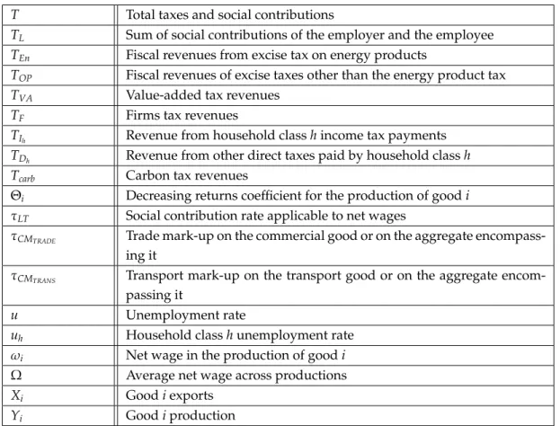
T Total taxes and social contributions
TL Sum of social contributions of the employer and the employee
TEn Fiscal revenues from excise tax on energy products
TOP Fiscal revenues of excise taxes other than the energy product tax
TVA Value-added tax revenues
TF Firms tax revenues
TIh Revenue from household class h income tax payments TDh Revenue from other direct taxes paid by household class h Tcarb Carbon tax revenues
⇥i Decreasing returns coefficient for the production of good i
⌧LT Social contribution rate applicable to net wages
⌧CMTRADE Trade mark-up on the commercial good or on the aggregate encompass-ing it
⌧CMTRANS Transport mark-up on the transport good or on the aggregate encom-passing it
u Unemployment rate
uh Household class h unemployment rate
!i Net wage in the production of good i
⌦ Average net wage across productions Xi Good i exports
Yi Good i production
Table 1 – Variables for solving Imaclim Argentina
1.2 Parameters calibrated on statistical data
Variable Name Description
L Total active population in full-time equivalents
Lh Active population of household class h in full-time equivalents
ij, Li, Ki Coefficients of theConstant Elasticity of Substitution (CES)production function governing the variables shares of conditional factor demands. Nh Total population of household class h.
NPh Number of retirees of household class h.
!OTh Share of the other transfers accruing to households devoted to house-hold class h.
!OTH Share of other transfers accruing to households (all classes together). Calibrated on the economic account table.
!OTF Share of other transfers accruing to firms. Calibrated on the economic account table (aggregate of financial and non financial firms, and of non-profit organisations).
!OTG Share of other transfers accruing to public administrations. Calibrated on the economic account table.
!Kh Share of the capital income of households accruing to household class h. Calibrated as the share accruing to household class h of revenues other than those of labour, in the m-class aggregation .
!KH Share of capital income accruing to households (all classes). Calibrated on the economic account table.
!KF Share of capital income accruing to firms. Calibrated on the economic account table (aggregate of financial and non financial firms, and of non-profit organisations).
!KG Share of capital income accruing to public administrations. Calibrated on the economic account table
⇡i Mark-up rate of profit margins(rate of net operating surplus) in the
production of good i. Calibrated as the ratio of net operating surplus to distributed output.
tOPTi Excise taxes other than the energy product tax per unit of consumption of good i. Calibrated as the ratio of the corresponding fiscal revenue of each good i (input-output table data after subtraction of the energy product tax) to total domestic consumption in the no-policy equilibrium Yi0 + Mi0 Xi0 (exports are assumed to be exempted).
tEnTFCi energy product tax per toe of energy product consumptions by
house-holds. The energy product tax is isolated from other excise taxes. tEnTICi energy product tax per toe of energy product in intermediate
consump-tions. The energy product tax is isolated from other excise taxes. ⌧TIh E↵ective income tax rate of household class h. Calibrated as the ratio of
income tax payments to the before-tax gross disposable income. Both aggregates are distributed among household classes based on the shares observed in the h-class aggregation .
⌧TF E↵ective firms tax rate. Calibrated as the ratio of the firms tax fiscal revenue, to the share of the gross operating surplus (GOS) accruing to firms.
⌧SMICij Specific mark-up rate on intermediate consumptions (if i is not a hybrid
good then the rate is nil). Defined during the hybridisation procedure. ⌧SMCi Specific mark-up rate on household consumptions (if i is not a hybrid
good then the rate is nil). Defined during the hybridisation procedure. ⌧SMGi Specific mark-up rate on public consumptions (if i is not a hybrid good
then the rate is nil). Defined during the hybridisation procedure. Under the convention that public energy consumptions are nil.
⌧SMIi Specific mark-up rate on investment (if i is not a hybrid good then the
rate is nil). Defined during the hybridisation procedure.
⌧SMXi Specific mark-up rate on exports (if i is not a hybrid good then the rate
is nil). Defined during the hybridisation procedure.
⌧Sh Savings rate of household class h. Calibrated as the ratio of the savings of class h to its gross disposable income (Rh), with the data being derived
from all the main data sources.
⌧VATi Value-added tax rate applying to the final consumption of good i. Cali-brated on input-output table data by treating the VAT as a simple sales tax levied indi↵erently on C, G and i.
continued on next page
Table 2 – Calibrated parameters for Imaclim-Country
1.3 Exogenous parameters
Variable Name Description
!CPI Indexation coefficient of wage on consumer price in the wage curve. The value "0" stands for noindexation of wages on consumer price -wage curve is on nominal -wage. The value "1" stands for a complete indexation of the wage curve on consumer price.
ih Share of the good i consumption of household class h that corresponds to a basic need. Set for each good i at a level that defines a basic need equal to 80% of the real consumption of the class for which it is the lowest.
ICji Technical asymptote of the technical coefficient ↵ij.
Ki Technical asymptote of the capital intensity of good i.
Li Technical asymptote of the labour intensity of good i.
Mi Evolution rate of the import of good i excluding price e↵ect.
Xi Evolution rate of the export of good i excluding price e↵ect.
pMi Evolution rate of the pMiprice of imported good j.
pXi Evolution rate of the pXi price of exported good j. Li Labour productivity improvements of good i.
i Substitution elasticity of the variable shares of production factors. CRi Income-elasticity of household consumption of good i.
CPi Price-elasticity of household consumption of good i.
Mpi Elasticity of the ratio of imports to domestic production of good i, to the
corresponding terms of trade.
Xpi Elasticity of good i exports to the corresponding terms of trade.
wu Elasticity of the average net wage (nominal or real, see supra) to the unemployment rate.
tcarbIC Carbon tax on the carbon emissions of intermediate consumptions. tcarbFC Carbon tax on the carbon emissions of household consumptions.
continued on next page
2 Formulary of Imaclim-Country
2.1 General equation framework
The modeling framework boils down to a set of simultaneous equations to solve on each time frame from the base year until the time horizon studied, such as the set of equations 1 which distinguishes three kinds of component: (xi)i2[1...k] are the variables computed by the model, which represent the endogenous elements of the projected energy-economy picture, ( i)i2[1...l] are a set of exogenous parameters (some of them are calibrated at the base year and the other are non-calibrated and come from external sources) and ( fi)i2[1...k]are a set of exogenous functions. The ficonstraints are of two di↵erent natures: one subset of equations describes the accounting constraints that are necessarily verified to ensure the accounting system is properly balanced and the other subset translates the technical and economic choices. The equations of the model could be seen in di↵erent blocks as well: price system and income generation, institutional sectors accounts, production and households’ consumption trade-o↵s, and market balances. Thereafter, we will detail the complete set of equations following each block.
8i 2 [1 . . . k], fi(x1, . . . ,xk, 1, . . . , l) = 0
In this set of equations, the calibrated parameters are identified with an over-line, the initial value for the resolution on each time frame with exponent 0 and the base year variables with exponent BY. Although equations are written in a generalized n-goods and m-households’ groups format.
2.2 Growth engine
In its basic version, Imaclim-Country projects the economy in the medium to long run in successive steps of resolution and relies on the method of comparative statics. Hereafter, t gives the time step between the base year and the year of resolution. The growth engine is basically exogenous and technical progress is implemented through factor augmenting coefficients (see Equations33,34, and35). It combines several drivers:
• The total population and active population growth:
NL = (1 + NL)t· N0 (2) • The implicit capital accumulation computed through a proportional link between total fixed capital consumption and the current level of total investment in capital good (see Equation62)
2.3 Producer and Consumer Prices
pYi the producer price of good i is built following the cost structure of the production of good i , that is as the sum of intermediate consumptions, labor costs, capital costs, a tax on production, and a constant mark-up rate (corresponding to the net operating surplus):
pYi = n X
j=1
pICi · ↵ij+pLi · li+pKi · ki+⌧Yi· pYi +⇡i· pYi (3)
The pMi price of imported good j is good-specific and the international composite good is the numéraire of the model; its price is assumed constant and equal to unity.
pMcomp =pMcomp0 = 1 (4)
The prices of others goods evolve according to an exogenous rate pMi: pMi =
⇣
1 + pMi ⌘t
· pMi0 (5)
The pMi parameters is used to simulate alternative world energy prices scenarios.
The average price piof the resource of good i is the weighted average of the two previous prices:
pYi · Yi+pMi · Mi
Yi+Mi (6)
The domestic and foreign varieties of the energy goods are indeed assumed homogeneous: the alternative assumption of product di↵erentiation, adopted by manycomputable general equilibrium (CGE) model through their use of an Armington specification for international trade (Armington, 1969), has the disadvantage of creating ’hybrid’ good varieties, whose volume unit is independent from that of the foreign and national varieties they hybridize; this forbids to maintain an explicit accounting of the physical energy flows and thus an energy
balance. For the sake of simplicity, the non-energy goods are treated similarly. pICi the price of good i consumed in the production of good j is equal to the resource price of good i plus trade and transport margins, specific margins, a domestic excise on oil products (energy product tax, EnT) , an aggregate of other excise taxes and a carbon tax which equal zero for this paper.
pICi =pi· (1 + ⌧CMi +⌧TMi+⌧SMICi) + tEnTICi +tOPTi+tcIC · ICij (7) The consumer price of good i for households pCi, public administrations (pGi) and investment (pIi), and the export price of good i (pXi), are constructed similarly and only di↵er on whether they are subject to value-added tax (the same rate is applied to all consumptions of one good) and the carbon tax or not. The latter tax applies to household prices only, as national accounting makes households the only final consumer of energy goods.
pCi = [pi· (1 + ⌧CMi +⌧TMi+⌧SMCi) + tEnTFCi +tOPTi +tcFC· FCij] · (1 + ⌧VATi) (8) pGi = [pi· (1 + ⌧CMi +⌧TMi+⌧SMGi) + tOPTi] · (1 + ⌧VATi) (9) pIi = [pi· (1 + ⌧CMi +⌧TMi+⌧SMIi) + tOPTi] · (1 + ⌧VATi) (10)
pXi =pi· (1 + ⌧CMi +⌧TMi +⌧SMXi) + tOPTi (11)
Trade margins ⌧CMi and transport margins ⌧TMi , identical for all intermediate and final consumptions of good i, are calibrated at the reference equilibrium and kept constant-except those on the productions aggregating transport and trade activities (hereafter indexed TRADE and TRANS), which are simply adjusted, in the derived equilibrium, to have the two types of margins sum up to zero :
n X
j=1
⌧CMTRADE· pTRADE· ↵TRADEj +⌧CMTRADE· pTRADE· (CTRADE+GTRADE+ITRADE+XTRADE)
+ n X i,TRADE n X j=1 ⌧CMi · pi· ↵ij· Yj+ X i,TRADE ⌧CMi· pi· (Ci+Gi+Ii+Xi) = 0 (12) and similarly: n X j=1
⌧CMTRANS · pTRANS· ↵TRANSj +⌧CMTRANS · pTRANS· (CTRANS+GTRANS+ITRANS+XTRANS)
+ n X i,TRANS n X j=1 ⌧CMi· pi· ↵ij· Yj+ X i,TRANS ⌧CMi · pi· (Ci+Gi+Ii+Xi) = 0 (13)
⌧LTi calibrated at base year:
pLi = (1 +⌧LTi) · !i (14)
In some versions, ⌧LT adjusts following either tax revenues, or any other public budget constraint (see Section2.9).
The net wage !ivaries as the average wage ⌦ : !i = ⌦
⌦BY · !iBY (15)
The average wage ⌦, subject to variations dictated by the labor market, being defined as: ⌦ = Pn i=1!i· li· Yi Pn i=1li· Yi (16)
The cost of capital is understood as the cost of the ’machine’ capital (see the description of the production trade-o↵s). It is obtained as the average price of investment goods.
pK = Pn i=1pIi · Ii Pn i=1Ii (17)
The consumer price index CPI is computed following Fisher, i.e. as the geometric mean of the Laspeyres index and the Paasche index.
CPI = s Pn i=1(pCi · Ci0) ·Pni=1(pCi · Ci) Pn i=1(pCi0· Ci0) ·Pni=1(pCi0 · Ci) (18) 2.4 Households
Households can be disaggregated into m classes (index h, h 2 [1, m]) to take into account income structures and eventually behaviors and adaptation capacities that can vary signifi-cantly from one household to the next. If there is no information on, or no use for household disaggregation The current Imaclim-ARG version does not inform any disaggregation and has a single consumption group for households. For the sake of a generalized formulary, we maintain the h index.
2.4.1 Income formation, savings and investment decision
The gross primary income of class h, or revenue before tax RBThis defined as the addition and the subtraction of the following terms:
• A share !Lh of the sum of aggregate endogenous net wage income !iliYi , which varies with the number of active people employed in each class.
• A share !Kh of the fraction of ’capital income’(the gross operating surplus of national accounting) that goes to households, GOSH (Equation 21). !Kh are exogenous and, if applied, their calibration is based on household consumption surveys and the economic account table.
• Social transfers, in three aggregates: both the pensions benefits (RPh) and the unemploy-ment benefits (RUh) following the average wage variation to BY, and the other social benefits (ROSBh) following the evolution of GDP per capita (N).
• An exogenous share !OTh of residual transfers OTH , which correspond to the sum of "other current transfers" and "capital transfers".
• A ’debt service’ iHDh, which corresponds to property income (interests, dividends, real estate revenues, etc.). This service is the product of the households’ net debt Dh , the evolution of which is explained below (Equation 26), and an e↵ective interest rate iH calibrated at BY. Hence, RBTh=!Lh n X i=1 !iliYi+!KhGOSH+RPhBY·!! BY+RUhBY· ! !BY+ROSBhBY· GDP N GDPBY NBY +!OThOTH ihDh (19) with in particular OTH and GOSH defined as constant shares !OTH and !KH of OT (equation (60)) and GOS (Equation36) :
OTH =!OTHOT (20)
GOSH =!KHGOS (21)
The gross disposable income Rhof class h is obtained by subtracting from RBThthe income tax TIhlevied at a constant average rate (Equation43), and other direct taxes TDhthat are indexed on CPI (Equation44). REXPh, the consumed income of class h, is inferred from disposable income by subtracting savings which is a proportion of the gross disposable income. The savings rate ⌧Sh is calibrated at BY.
Rh=RBTh TIh TDh (22)
REXPh = (1 ⌧Sh) Rh (23)
A further exploration of the data available in the economic account table gives households’ investment GFCFh (Gross Fixed Capital Formation) as distinct from their savings; GFCFh is assumed to follow the simple rule of a fixed ratio to gross disposable income (Equation25). The di↵erence between savings and investment gives the self-financing capacity of class h: AFCh. GFCFh Rh = GFCFh0 Rh0 (24) AFCh=⌧ShRh GFCFh (25)
The evolution of AFCh can then be used to estimate the evolution of net debt Dh . The computation is based on the simple assumption of a gradual wedge of AFC at each step of resolution.
Dh=Dh0 + t+1 t2 (AFCh0 AFCh) (26)
2.4.2 Consumption
The consumption of households, for each good i, has been defined, without resorting to any explicit utility function, as the sum of a exogenous basic needs, common to all classes, and a consumption in excess of this need that varies according to some income elasticity CRi , and some price-elasticity CPi . For the time being these elasticities come from literature reviews.
f or i , composite, Cih = ihCih0 + ⇣ 1 ih ⌘ 0BBBB @CPI ·pCi p1C i0 1 CCCC A CPi 0 BBBB
@RCPI ·EXPh REXP1 h0 1 CCCC A CRi Cih0 (27) where ih represents the share of the reference consumption of class h that corresponds to a basic need, and with prices indexed in the same way as the consumptions they value.
For a given good i, Equation27can be substituted, at each time step, by exogenous infor-mation coming from bottom-up models. For example, we can inform exogenous trajectories of energy consumption for households.
The demand for the composite good (that aggregates the rest of the economy) of class h is then simply defined as the balance of the class’s consumed income-which amounts to imposing
a binding budget constraint. Ccomph =REXPh X j,comp ⇣ pjCj ⌘ (28)
2.5 Production (institutional sector of firms)
2.5.1 Gross disposable income and investment decision
Similar to households, the firms’ disposable income RF is defined as the addition and subtraction of:
• an exogenous share !KSof capital income i.e. GOS (Equation36),
• a ’debt service’ (interests, dividends) iFDFand served at an interest rate iFcalibrated at BY,
• corporate tax payments TF,
• and an exogenous share !OTF of other transfers OT, which are assumed a constant share of GDP (Equation60).
RF=!KSGOS iFDF TF+!OTFOT (29)
The ratio of the gross fix capital formation of firms GFCFFto their disposable income RFis assumed constant; same as for households and in accordance with national accounting their self-financing capacity AFCFthen arises from the di↵erence between RFand GFCFF. The net debt of firms DSis then calculated from their AFCF on the same reasoning as that applied to households. GFCFF RF = GFCFF0 RF0 (30) AFCF=RF GFCFF (31) DF=DF0 + t+1 t2 (AFCF0 AFCF) (32) 2.5.2 Production trade-o↵s
The production trade-o↵s, which are the subject of a specific publication (Ghersi and Hour-cade,2006), assume technical asymptotes that constrain the unit consumptions of factors above
some floor values. The restrictive assumption is made that the variable shares of the unit con-sumptions of each factors (secondary inputs, labor and capital) are substitutable according to a CES specification: the existence of a fix share of each of these consumptions implies that the elasticities of substitution of total unit consumptions (sum of the fix and variable shares) are not fixed, but decrease as the consumptions approach their asymptotes. Under these assumptions and constraints, the minimization of unit costs of production leads to a formulation of the unitary consumptions of secondary factors ↵ji, of labor liand of capital kiwhich can be written as the sum of the floor value and a consumption above this value. The latter corresponds to the familiar expression of conditional factor demands of a CES production function with an elasticity of i(the coefficients of which, ICij, Li0 and Ki0 , are calibrated at BY).
↵ji= 2 6666 6666 4 ICji↵ji0 + ji pICji ! i 0 BBBB BB@ n X j=1 jii pICji1 i+ Lii (1 +pLi i)t 1 i + Kii pKi1 i 1 CCCC CCA 1 ⇢i37777 7777 5 (33) li = 2 6666 6666 4 Lili0 + Li pLi ! i 0 BBBB BB@ n X j=1 jii pICji1 i+ Lii (1 +pLi i)t 1 i + Kii pKi1 i 1 CCCC CCA 1 ⇢i37777 7777 5 (34) ki = 2 6666 6666 4 Kiki0 + Ki pKi ! i 0 BBBB BB@ n X j=1 jii pICji1 i+ Lii (1 +pLi i)t 1 i + Kii pKi1 i 1 CCCC CCA 1 ⇢i37777 7777 5 (35)
where for convenience:
⇢i= i 1 i
The exogenous labor productivity improvements iis implemented as factor augmenting productivity gains. It makes it possible to drive changes in production patterns to mimic specific economic scenarios.
Let emphasize again that the ’cost of capital’ pK entering the trade-o↵s is ‘stricto sensu’ the price of ’machine capital’, i.e. equal to a simple weighted sum of the investment prices of immobilized goods (Equation17), and unrelated to the interest rates charged on financial markets: on the one hand production trade-o↵s are based upon the strict cost of inputs, including that of physical capital ki(calibrated on the consumption of fixed capital of the input-output table); on the other hand, regardless of this arbitrage, the firm’s activity and a rule of self-investment (GFCFF, Equation30) lead to a change in financial position DF, whose service is not assumed to specifically weigh on physical capital as an input.
A peculiarity of the Imaclim-Country modeling is that these results intensities of factors can be substituted by information coming from technical-economic models. For example, we can inform the capital or labor intensity for a sector i such as the electricity sector, at di↵erent
time steps of the resolution, just as we can inform the energy intensities of all sectors of the economy. Thanks to the hybridization procedure, there is consistency in embedding an energy intensity calculated on volumes in the Imaclim-Country model. In addition, it is also possible to directly inform volumes. In this case, the intensity will be determined endogenously as defined.
2.5.3 Gross operating surplus
Trade-o↵s in the i productions, constant rates of operating margin ⇡iand specific margins ⌧SMdetermine the gross operating surplus (GOS) :
GOS = n X i=1 ⇣ pKikiYi+⇡ipYiYi ⌘ +SM (36)
This GOS, that corresponds to capital income, is split between agents following constant shares (calibrated at BY). By construction, the specific margins on the di↵erent sales SM sum to zero at BY (this is a constraint of the hybridization procedure by building the database), however they do not sum to zero in runs, their constant rates being applied to varying prices. Their expression is then:
SM =X
i 0 BBBB
BB@Xj ⌧SMICijpi↵ijYj + ⌧SMCipiCi+⌧SMGipiGi +⌧SMXipiXi 1 CCCC
CCA (37)
2.6 Public administrations
2.6.1 Tax, social security contributions and fiscal policy
Tax and social security contributions give the larger share of government resources. In most versions of the model, tax rates and excise taxes other than the carbon tax and social contributions are supposed constant, and the various tax revenues are defined by applying
these rates to their respective bases: TY= n X i=1 ⌧YipYiYi (38) TEn= n X i=1 n X j=1 tEnT ICji↵jiYi+ n X i=1 tEnT FCi(Ci+Gi+Ii) (39) TOP= n X i=1 n X j=1 tOPTj↵jiYi+ n X i=1 tOPTi (Ci+Gi+Ii) (40) TVA= n X i=1 ⌧VATi 1 + ⌧VATi ⇣ pCiCi+pGiGi+pIiIi ⌘ (41) TF=⌧TFGOSF (42) TIh =⌧TIhRBTh (43) TDh =CPI · TDh0 (44)
Fiscal revenues of the carbon tax Tcarb(if applied) and the sum of labor tax (social insurance contributions and benefits) TLare computed following the same logic:
TL=⌧LT n X i=1 wiliYi (45) Tcarb= n X i=1 n X j=1 tcarbIC ICji↵jiYi+ n X i=1 tcarbFC FCiCi (46)
The carbon tax on intermediate consumptions (tcarbIC) and on final consumptions (tcarbFC) are exogenous (see Section).
2.6.2 Gross disposable income, public spending, investment and transfers
Similar to households and firms (following the logic prevailing in the economic account table), the gross disposable income of public administrations RGis the sum of taxes and social contributions, of exogenous shares !KG of GOS and !OTG of ’other transfers’ OT , from which are subtracted public expenditures pGG , a set of social transfers RP , RUand ROSB, and a debt service iGDG: RG=T + !KGGOS + !OTGOT n X i=1 pGiGi RP RU RO iGDG (47)
Public expenditures pGG are assumed to keep pace with national income, and therefore are constrained as a constant share of GDP:
n P i=1pGiGi GDP = n P i=1pGi0Gi0 GDP0 (48)
Social transfers RP, RUand ROare the sum across household classes of the transfers defined as components of their before-tax disposable income (Equation19) :
RP= m X h=1 NPh⇢Ph (49) RU = m X h=1 NUh⇢Uh (50) ROSB= m X h=1 Nh⇢Oh (51)
With per capita transfers ⇢Ph , ⇢Uh and ⇢Oh indexed on the average net wage: 8 K 2 [P, U, OSB], 8 h 2 [1, m] ⇢Kh = ww
0⇢Kh0 (52)
At last, the interest rate iGof public debt evolves as do iHand iF(Equation ?? ). Public investment GFCFG, same as public expenditures pGG, is supposed to mobilize a constant share of GDP. Subtracting it from RGgives AFCG, which determines the variation of the public debt:
GFCFG GDP = GFCFG0 GDP0 (53) AFCG=RGDG GFCFG (54) DG=DG0 t+1 t2 (AFCG0 AFCG) (55)
2.7 "Rest of the World"
2.7.1 Balance of Trade
Concerning international trade the assumption is made of an open economy whose weight does not a↵ect world prices: global import prices pMretain their relative values (Equation5). Then the ratio of imports to domestic production on the one hand, and the ’absolute’ exported quantities on the other hand, are elastic to the terms of trade, according to fixed good-specific
elasticities : Mi Yi = 1 + Mi t· Mi0 Yi0 0 BBBB @ pMi0 pYi0 pYi pMi 1 CCCC A Mpi (56) Xi Xi0 = 1 + Xi t· 0 BBBB @ pXi0 pMi0 pMi pXi 1 CCCC A Xpi (57)
The di↵erent treatment of imports and exports merely reflects the assumption that, notwith-standing the evolution of the terms of trade, import volumes rise in proportion to economic activity (domestic production), while exports do not (global demand is assumed constant). It implies, however, that improved terms of trade do not necessarily mean an improvement in the trade balance, depending on the concomitant variations of activity.
Eventually, exports are impacted by global economic growth, independently of terms of trade variations. This is captured by assuming an exogenous rate of growth of exports Xi. Usually, for non-energy goods, this parameter follows world growth assumption over time. Outsourcing and relocations can be captured by the exogenous parameter Mi.
For hybrid goods in volume, Equations56and57can be substituted, at each time step, by exogenous information coming from bottom-up models. For example, we can inform the full exogenous trajectories of energy trade.
2.7.2 Capital flows and self-financing capacity
Capital flows from and to the ROW are not assigned a specific behavior, but are simply determined as the balance of capital flows of the three national institutional sectors (households, firms, public administrations) to ensure the balance of trade accounting. This assumption determines the self-financing capacity of the ROW, which in turn determines the evolution of DROW, its net financial debt:
AFCROW= n X i=1 pMiMi n X i=1 pXiXi+ n X K=H, S, G iKDK n X K=H, S, G OTK (58)
DROW=DROW0 + t+1 t2 (AFCROW0 AFCROW) (59) By construction the self-financing capacities (AFC) of the four agents clear (sum to zero), and accordingly the net positions, which are systematically built on the AFCs, change from a position in which they are strictly compensating each other to another such position. Indeed a nil condition on the sum of net positions could be substituted to Equation59without impacting the results of the model. The hypothesis of a systematic ’compensation’ by the ROW of the
property incomes of national agents without any reference to its debt DROWmay seem crude, but in fine only replicates the method of construction of the economic account table. Indeed, in the no-policy equilibrium the e↵ective interest rate of the ROW (ratio of net debt to its property income), which ultimately results from a myriad of debit and credit positions and from the corresponding capital flows, is negative, so unworkable for modeling purposes.
To conclude, as previously mentioned other transfers OT ("other current transfers " and "capital transfers ") are defined as a fixed share of GDP :
OT GDP = OT0 GDP0 (60) 2.8 Market balances 2.8.1 Goods markets
Goods market clearing is a simple accounting balance between resources (production and imports) and uses (households and public administrations’ consumption, investment, exports). Thanks to the process of hybridization, this equation is written in volume for hybrid goods. For energy goods it is written in Mtoefor energy goods and consistent with the energy balance used (the G and I of these goods are nil by definition).
Yi+Mi =Ci+Gi+Ii+Xi (61)
2.8.2 Investment and capital flows
Contrary to standard CGE models, Imaclim-Country does not represent explicit capital markets, which is admissible given the nature of static exercises conducted. The capital-investment balance is "demand-driven". As previously highlighted, productive sectors arbi-trate capital consumption according to prices of equipment, and not according to the return on capital.
Then, the capital immobilized in all productions is supposed homogeneous, and all its components vary as the total consumption of fixed capital:
Ii Pn j=1kj· Yj = i = Ii0 Pn j=1kj0 · Yj0 (62)
In the meantime, the assumption is made of a single investment good in the economy as a weighted sum of di↵erent goods calibrated at base year.
Commonly, in Imaclim-Country and other CGE models, the investment is a vector: it informs for each sector its investment within the overall economy. It makes it difficult to undertake a robust evaluation of the impacts on structural changes in contrasted investment plans for a specific sector j. This is why a specific modeling approach can be set up by describing a complete investment matrix Iijat calibration (thanks to capital breakdown literature). Instead of being of vector dimension, Equation 62 is then of matrix dimension, but the modeling constraint remains the same. However, for each time step, it allows us to specify the demand for investment -by sector- generated by the sector j. This specification is used to model contrasted investment in the power sector’s technologies.
Furthermore, the investment supply adapts to the demand. Capital formation from firms completes households and public contribution to satisfy that demand, and, balance investment flows. GFCFH+GFCFF+GFCFG= n X i=1 pIi · Ii (63)
Eventually, the investment balance, together with households saving rate and public ex-penses, imposes the external or trade balance which is endogenous in the model.
2.8.3 Employment
The labor market conditions, results from the interplay between labor demand from the production systems, equal to the sum of their factor demands liYi , and of labor supply from households. As part of key structural assumptions, the model allows for a strictly positive unemployment rate u and the market balance writes:
(1 u) NL = n X
i=1
liYi (64)
Rather than explicitly describe labor supply behavior, the model infers changes in u fol-lowing a wage curve, which describes an empirical correlation between the average real wage ⌦ and the unemployment rateu, characterized by an constant elasticity wu. The underlying intuition is that any increase in unemployment creates a downward pressure on wages, which is indeed interpretable in terms of either bargaining power, or efficiency wage:
⌦
wCPIi · CPI + (1 wCPIi) = ⌦0· ✓ u
u0 ◆ wu
There is also the possibility of setting a sectoral wage curve. It takes the same formulation as the previous equation but uses the net wage of sector !i. In this configuration, Equation15is removed from the system. The indexation parameter wCPIi gives a flexibility to describe a wage curve based either on nominal wage ( wCPIi = 0) or real wage ( wCPIi = 1). For all values included between 0 and 1, we assume that only a share of wage can be bargain based on real wage. The underlying intuition is that any increase in unemployment creates a downward pressure on wages, which is indeed interpretable in terms of either bargaining power, or efficiency wage. According to the openness of the economy (or the sectors for a sectoral wage curve) at the international scale and its mobility, the bargain lies between real wage and nominal wage.
If di↵erent household classes are represented, changes in employment corresponding to the evolution of u are then split between the classes according to their specific unemployment uh:
uh=uh0 uu
0 (66)
2.9 Carbon tax policies
The model is specifically designed to study carbon tax policies in the medium to long run by generating policy-constrained projections. In the model, implementing a carbon tax amounts to adding a shock on energy prices proportional to their carbon content at the time horizon studied.
The implementation of carbon prices1(t
carbIC and tcarbC) increase intermediate consumption prices (Equation 7) and purchaser’s price for households (Equation 7) in proportion of the emission factor of the energy good i consummed by sector j ( ICij), and households ( Ci)2.
In the present model version, Imaclim-Country can simulate di↵erent uses of the carbon tax revenues Tcarb, that can be split in three categories. The carbon tax revenues is either used:
• to only feed public budget, or
• to directly compensate domestic agents: firms and/or households, or • to reduce existing other taxes rates.
The recycling options can be combined: a share of the carbon tax revenues may be directly returned to domestic agents, and the remained part is then used to reduce other taxes rates.
Direct compensations can be computed by the following constraints: 1The framework can accommodate sector specific carbon prices.
• Lump-sum transfer to households
A share ( LSH) of the carbon tax revenues are directly transferred to households while maintaining neutral policy budget:
LSH = LSH· Tcarbwith LSF 2 [0, 1] (67)
• Lump-sum transfer to firms
A share ( LSF) of the carbon tax revenues are directly transferred to firms while maintain-ing neutral policy budget:
LSF= LSF· Tcarb with LSF 2 [0, 1] (68)
The shares LSH and LSF can be fixed exogenously as a parameters or can correspond to a proportion of variables, endogenously. For no direct transfers to agents, the shares are set up to zero.
Carbon tax revenues can be used to alleviate di↵erent existing taxation. We focus on a standard case: the reduction of the labor tax that can be set up under di↵erent constraints:
• All carbon tax revenues (net of direct compensation if also applied) are used to reduce the labor taxation while maintaining neutral policy budget. Thus, under this recycling option, the sector specific rates of labor taxes ⌧TLis alleviated by the same coefficient TL:
Tcarb LSH LSF= TL n X i !i· li· Yi (69) with ⌧TL =⌧TL + TL (70)
• The level of labor tax reduction is determined while imposing a specific budget constraint. Thus, the cut TL is endogenously calculated to satisfy the budget condition.
Unless otherwise specified, carbon tax implementations are recycled into labor tax re-duction while maintaining the government financial capacity constant to GDP variation:
AFGG
GDP =
AFGG0
GDP0 (71)
3 The accounting framework
All interactions are synthesised in a large accounting framework composed by two tables. • The Input-Output table balances the uses and resources of products (see Table4). Each
sector produces one single good so that commodities and activities match and the Input-Ouput table (IOT).
• The national economic accounts table details the primary and secondary distribution of income between representative economic agents (see5). The model distinguishes four economic agents : households (H)3, corporate firms (F), public administrations or government (G) and the rest of the world (ROW).
Imaclim Brazil keeps detail on primary income distribution between each economic agents. Therefore households, firms and government have separated accounts in our model and may have di↵erent structural behaviours. This is an extention to traditional framework of CGE
models that usually shortcut this aspect by assuming that households eventually own the total endowment of production factors. Households are the only agent to own labour factor.
Furthermore, through secondary income distribution, economic agents break down their income between goods consumption, investment, tax payments and transfers. The model considers a detailed system of taxes and transfers essentially between the triangle of domestic agents (households, firms and public administrations). This will be detailed in the following.
Owing to the split of accounts of institutional agents, Imaclim Brazil also considers the breakdown of totalGross Fixed Capital Formation (GFCF)between agents. It further identifies for each agent the share of income that is not directly invested inGFCF, which is called self-financing capacity (ACF). The rest of the world classically interacts with domestic agents through trade of goods and capital balance.
The rest of this section details the equations of the model through di↵erent blocks: (i) price system and income generation, (ii) institutional sectors accounts, (iii) production and consumption trade-o↵, (iv) market balances, (v) growth engine, (vi) carbon tax policies.
The equations of the model are of two quite di↵erent natures: one subset of equations describes accounting constraints that are necessarily verified to ensure that the accounting system is properly balanced; the other subset translates various behavioural constraints, written either in a simple linear manner (e.g. households consume a fixed proportion of their income) or in a more complex non-linear way (e.g. the trade-o↵s of production and consumption). It is these behavioural constraints that ultimately reflect a certain economic worldview.
Intermediate consumption (IC val ij ) Final Consumption (FC val i ) Uses (U sei ) Hybrid sectors Non-hybrid sectors Households (Cval i ) Public administration (Gval i ) Investment (Ival i ) Exports (Xval i ) Intermediate consumption (IC valij ) Hybrid sectors pICij ·↵ij ·Y j pICij ·↵ij ·Y j pCi ·Ci pGi ·Gi pIi ·Ii pXi ·Xi P IC j val ij + FC val i Non-hybrid sectors pICij ·↵ij ·Y j pICij ·↵ij ·Y j pCi ·Ci pGi ·Gi pIi ·Ii pXi ·Xi P IC j val ij + FC val i V alue-added (VA j ) Labour income !j ·lj ·Yj !j ·lj ·Yj Labour Tax ⌧TL ·! j ·lj ·Y j ⌧TL ·! j ·lj ·Y j Capital income pKj ·kj ·Yj pKj ·kj ·Yj Pr oduction Tax ⌧TY i ·pY j ·Yj ⌧TY i ·pY j ·Yj Pr ofit mar gin ⇡j ·pY j ·Yj ⇡j ·pY j ·Yj Production (Yval j ) pYj ·Y j pYj ·Y j Imports (M val j ) pMj ·M j pMj ·M j Margins (Mar gj ) Trade mar gins ⌧CM j ·pj ·( Yj + Mj ) ⌧CM j ·pj ·( Yj + Mj ) Transport mar gins ⌧TM j ·pj ·( Yj + Mj ) ⌧TM j ·pj ·( Yj + Mj ) Specific mar gins on IC (SM ICij ) ⌧SM ICij ·pj ·↵ji ·Yj 0 SpeMar g on C (SM Cj ) ⌧SM Cj ·pj ·Cj 0 SpeMar g on G (SM Gj ) ⌧SM Gj ·pj ·G j 0 SpeMar g (SM Ij ) ⌧SM I j ·pj ·Ij 0 SpeMar g (SM Xj ) ⌧SM Xj ·pj ·X j 0 Taxes (Tj ) Value-added tax ( ⌧V AT j 1 ⌧V AT j )· FCval j ( ⌧V AT j 1 ⌧V AT j )· FCval j Ener gy Tax IC tEnT ICj · P (↵ i ji ·Yi ) tEnT ICj · P (↵ i ji ·Yi ) Ener gy Tax FC tEnT FC j ·( Cj + Gj + Ij ) tEnT FC j ·( Cj + Gj + Ij ) Other indir ect tax on pr oducts tOPT j ·( P ↵ i ji ·Yi + Cj + Gj + Ij ) tOPT j ·( P ↵ i ji ·Yi + Cj + Gj + Ij ) Supply (Sup j ) Yval j + Mval j + Mar gj + Tj + Tj Yval j + Mval j + Mar gj + Tj + Tj Table 4 – Imaclim -C ountr y Input-Output table (IOT)
Firms (F ) Public administration (G ) Households (H ) Rest of world (ROW ) Trade balance -P (p i Mi ·M i pXi ·Xi ) Gr oss operating surplus (GO S) 4 !K F ·GOS !K G ·GOS !K H ·GOS -Labour income -P (! j j ·lj ·Y j ) -Labour tax (TL ) -⌧TL P (! j j ·lj ·Y j ) -Pr oduction tax (T Y ) -P ⌧ j TY j ·pY j ·Y j -Ener gy tax (TEn ) -P [t j EnT ICj · P (↵ i ji ·Yi )+ tEnT FC j ·( Cj + Gj + Ij )] -Other indir ect tax (TOP ) -P [t j OPT j ·( P ↵ i ji ·Yi + Cj + Gj + Ij )] -V alue-added tax (TVA ) -P [( j ⌧V AT j 1 ⌧V AT j )· FCval j ] -Pr operty income iF ·D F iG ·D G P (i h h ·D h ) iF ·D F + iG ·D G + P (i h h ·D h ) Unemployment transfers (U ) -P (⇢ h Uh ·N Uh ) P (⇢ h Uh ·N Uh ) -Pensions (P ) -P (⇢ h Ph ·N Ph ) P (⇢ h Ph ·N Ph ) -Other social transfers (O ) -P (⇢ h Oh ·N Oh ) P (⇢ h Oh ·N Oh ) -Other transfers (OT ) !OT F ·OT !OT G ·OT !OT H ·OT (!OT F ·OT + !OT G ·OT + !OT H ·OT ) Income tax (TI H ) -P (⌧ h TI h ·RBT h ) P (⌧ h TI h ·RBT h ) -Firm tax (TF ) ⌧TF ·GOS F ⌧TF ·GOS F -Other dir ect tax (TD ) -P (⌧ h TDh ·CPI ) P (⌧ h TDh 0 ·CPI ) -Gross disposable income (R ) RF = P row below RG = P row below RH = P row below RROW = P row below Final consumption (FC val ) -P G i val i RCON SH = P (1 h ⌧Sh )· Rh -Gr oss fixed capital consumption (GFCF ) GFCF F = GFCF F 0 RF 0 ·RF GFCF G = GFCF G0 GDP 0 ·GDP GFCF H = P ( h GFCF h 0 Rh 0 ·Rh ) -Expenses for final uses GFCF F P G i vali + GFCF G RCON SH + GFCF H -Self-financing capacity (AFC ) AFC F = RF GFCF F AFC G = RG [GFCF G + P G i val i ] AFC H = P (⌧ h Sh ·Rh GFCF h ) ACF ROW = (AFC F + ACF G + ACF H ) Net financial debt (D ) DF = DF 0 + tref ·(2 AFC F0 ACF F ) DG = DG 0 + tref 2 ·( AFC G0 ACF G ) DH = DH 0 + tref 2 ·( AFC H0 ACF H ) DROW = (DF + DG + DH ) Table 5 – Imaclim -C ountr y national economic accounts table
Bibliography
Armington, P.S., 1969. A Theory of Demand for Products Distinguished by Place of Production. International Monetary Fund Vol. 16, N, pp. 159–178.
Ghersi, F., Hourcade, J.C., 2006. Macroeconomic Consistency issues in E3 Modeling: The Continued Fable of the Elephant and the Rabbit. The Energy Journal SI2006, 39–62. doi:10. 5547/ISSN0195-6574-EJ-VolSI2006-NoSI2-3.
Le Treut, G., Combet, E., Lefèvre, J., Teixeira, A., Baudin, A., 2019. IMACLIM-Country platform : a country-scale computable general equilibrium model. URL:https://zenodo.org/record/ 3403961, doi:10.5281/ZENODO.3403961.