Visualization of data structure, domain knowledge and data mining results: application to breast cancer gene expressions

https://doi.org/10.4224/5764227

READ THESE TERMS AND CONDITIONS CAREFULLY BEFORE USING THIS WEBSITE. https://nrc-publications.canada.ca/eng/copyright

Vous avez des questions? Nous pouvons vous aider. Pour communiquer directement avec un auteur, consultez la

première page de la revue dans laquelle son article a été publié afin de trouver ses coordonnées. Si vous n’arrivez pas à les repérer, communiquez avec nous à PublicationsArchive-ArchivesPublications@nrc-cnrc.gc.ca.

Questions? Contact the NRC Publications Archive team at

PublicationsArchive-ArchivesPublications@nrc-cnrc.gc.ca. If you wish to email the authors directly, please see the first page of the publication for their contact information.

NRC Publications Archive

Archives des publications du CNRC

For the publisher’s version, please access the DOI link below./ Pour consulter la version de l’éditeur, utilisez le lien DOI ci-dessous.

Access and use of this website and the material on it are subject to the Terms and Conditions set forth at

Visualization of data structure, domain knowledge and data mining

results: application to breast cancer gene expressions

Valdés, Julio; Barton, Alan

https://publications-cnrc.canada.ca/fra/droits

L’accès à ce site Web et l’utilisation de son contenu sont assujettis aux conditions présentées dans le site LISEZ CES CONDITIONS ATTENTIVEMENT AVANT D’UTILISER CE SITE WEB.

NRC Publications Record / Notice d'Archives des publications de CNRC:

National Research Council Canada Institute for Information Technology Conseil national de recherches Canada Institut de technologie de l'information

Visualization of Data Structure, Domain

Knowledge and Data Mining Results:

Application to Breast Cancer Gene

Expressions *

Valdés, J., Barton, A.

2006

* published as NRC/ERB-1136. 11 pages. 2006. NRC 48489.

Copyright 2006 by

National Research Council of Canada

Permission is granted to quote short excerpts and to reproduce figures and tables from this report, provided that the source of such material is fully acknowledged.

National Research Council Canada Institute for Information Technology Conseil national de recherches Canada Institut de technologie de l’information

V isua liza t ion of Da t a St ruc t ure ,

Dom a in K now le dge a nd Da t a M ining

Re sult s: Applic a t ion t o Bre a st

Ca nc e r Ge ne Ex pre ssions

Valdés, J., Barton, A.

2006

Copyright 2006 by

National Research Council of Canada

Permission is granted to quote short excerpts and to reproduce figures and tables from this report, provided that the source of such material is fully acknowledged.

NRC 48489

Visualization of Data Structure, Domain Knowledge, and Data Mining Results:

Application to Breast Cancer Gene Expressions

Julio J. Vald´es and Alan J. Barton

National Research Council Canada

Institute for Information Technology

M50, 1200 Montreal Rd., Ottawa, Ontario, K1A 0R6

Canada

E-mail: julio.valdes@nrc-cnrc.gc.ca

alan.barton@nrc-cnrc.gc.ca

Abstract

Computational visualization techniques are used to explore, in an immersive fashion, inherent data structure in both an unsupervised and supervised manner. Supervision is provided via i) domain knowledge contained in breast cancer data, and ii) unsupervised data mining procedures, such as k-means and rough set based k-means. Despite no explicit preprocessing, exploration of high dimensional data sets is demonstrated. In particular, some of the visual perspectives presented in this study may be useful for helping to understand breast cancer gene expressions or results from computational data mining procedures.

Keywords: Biological Data Visualization, Biological Data Mining, Pattern Recognition, Microarray Data Analysis

1

Introduction

There are many computational techniques that may be used within a knowledge discovery process and applied to complex real world data sets. These various computations may lead to a plethora of data mining results, which, along with the data, need to be analyzed and properly understood. Humans are capable of visually perceiving large quantities of information at very high input rates; by far outperforming modern computers. Therefore, one approach to aid comprehension of large data sets (possibly containing space or time dependencies) and data mining results obtained from computer procedures, is to orient knowledge representations towards this vast human capacity for visual perception.

Several reasons make Virtual Reality (VR) a suitable paradigm for such a representation: Virtual Reality is flexible: it allows the choice of different representation models to better accommodate different human perception preferences. VR, it allows immersion: that is, the user can navigate inside the data, interact with the objects in the world, change scales, perspectives, etc. VR creates a living experience: the user is not merely a passive observer or an outsider, but an actor in the world, in fact. VR is broad and deep: the user may see the VR world as a whole, and/or concentrate the focus of attention on specific details or portions of the world. In order to interact with a Virtual World, no specialized knowledge is required.

This paper investigates some possible visual approaches when analyzing breast cancer data for the problems of under-standing i) the inherent structure of very high dimensional gene expression microarray data; from the gene and sample perspectives, ii) the results of data mining clustering procedures; such as the traditional k-means algorithm and a rough sets based version, and iii) the contribution of a supervised (versus unsupervised) visual representation.

2

Virtual Reality Representation Of Relational Structures

A virtual reality, visual, data mining technique extending the concept of 3D modelling to relational structures was in-troduced [14], [16], (see also http://www.hybridstrategies.com). It is oriented to the understanding of large

heterogeneous, incomplete and imprecise data, as well as symbolic knowledge. The notion of data is not restricted to data-bases, but includes logical relations and other forms of both structured and non-structured knowledge. In this approach, the data objects are considered as tuples from a heterogeneous space [15].

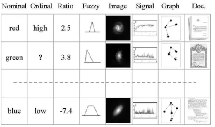
Figure 1. An example of a heterogeneous database. Nominal, ordinal, ratio, fuzzy, image, signal, graph, and document data are mixed. The symbol? denotes a missing value.

Different information sources are associated with the attributes, relations and functions, and these sources are associated with the nature of what is observed (e.g. point measurements, signals, documents, images, etc). They are described by mathematical sets of the appropriate kind called source sets (Ψi), constructed according to the nature of the information

source to represent (e.g. point measurements of continuous variables by subsets of the reals in the appropriate ranges, structural information by directed graphs, etc). Source sets also account for incomplete information. A heterogeneous domain is a Cartesian product of a collection of source sets: ˆHn _{= Ψ}

1× · · · × Ψn , wheren > 0 is the number of information

sources to consider. For example, in a domain where objects are described by attributes like continuous crisp quantities, discrete features, fuzzy features, time-series, images, and graphs (missing values are allowed). They can be represented as Cartesian products of subsets of real numbers( ˆR), nominal ( ˆN ) or ordinal sets( ˆO), fuzzy sets( ˆF ), set of images ( ˆI) , set of time series ( ˆS) and sets of graphs ( ˆG), respectively (all extended for allow missing values). The heterogeneous domain is

ˆ

Hn_{= ˆN}nN_{× ˆO}nO_{× ˆR}nR_{× ˆF}nF _{× ˆI}nI_{× ˆS}nS_{× ˆG}nG

, wherenN is the number of nominal sets,nOof ordinal sets,nRof

real-valued sets ,nFof fuzzy sets ,nI of image-valued sets,nSof time-series sets, andnGof graph-valued sets, respectively

(n = nN + nO+ nR+ nF+ nI+ nS+ nG).

A virtual reality space is the tupleΥ =< O, G, B, ℜm_{, g}

o, l, gr, b, r >, where O is a relational structure (O =< O, Γv>

, theO is a finite set of objects, and Γv _{is a set of relations),G is a non-empty set of geometries representing the different}

objects and relations. B is a non-empty set of behaviors of the objects in the virtual world. ℜm_⊂

R

m

is a metric space of dimensionm (euclidean or not) which will be the actual virtual reality geometric space. The other elements are mappings: go: O → G, l : O → ℜm,gr: Γv→ G, b : O → B.

Of particular importance is the mappingl. If the objects are in a heterogeneous space, l : ˆHn _{→ ℜ}m

. Several desiderata can be considered for building a VR-space. One may be to preserve one or more properties from the original space as much as possible (for example, the similarity structure of the data [4]). From an unsupervised perspective, the role ofl could be to maximize some metric/non-metric structure preservation criteria [3], or minimizing some measure of information loss. From a supervised point of viewl could be chosen as to emphasize some measure of class separability over the objects in O [16]. Hybrid requirements are also possible.

3

Nonlinear Discriminant Neural Networks

In the supervised case, a natural choice for representing thel mapping is a NDA neural network [19], [10], [11], [8]. One strong reason is the complex nature of the class relationships in complex, high dimension problems like gene expression data, where objects are described in terms of several thousands of genes, and classes are often either only separable with nonlinear boundaries, or not separable at all. Another is the generalization capabilities of neural networks which will allow the classification of new incoming objects, and their immediate placement within the created VR spaces. Of no less importance

is that when learning the mapping, the neural network hidden layers create new nonlinear features for the mapped objects, such that they are separated into classes by the output layer. However, these nonlinear features could be used independently with other data mining algorithms. The typical architecture of such networks is reported in [18].

NDA is a feedforward network with one or more hidden layers where the number of input nodes is set to the number of features of the data objects, and the number of neurons in the output layer to be the number of pattern classes. The number of neurons in the last hidden layer tom, the dimensionality of the projected space (for a VR space this is typically 3). From input layer to the last hidden layer, the network implements a nonlinear projection from original n-dimensional space to anm-dimensional space. If the entire network can correctly classify a linearly-nonseparable data set, this projection actually converts the linearly-nonseparable data to separable data. The backpropagation learning algorithm is used to train the feedforward network with two hidden layers in a collection of epochs, such that in each, all the patterns in the training data set are seen once, in a random order.

This classical approach to building NDA networks suffers from the well known problem of local extrema entrapment. In this paper a variant in the construction of NDA networks is used [18] by using hybrid stochastic-deterministic feed forward networks (SD-FFNN). The SD-FFNN is a hybrid model where training is based on a combination of simulated annealing with the powerful minima seeking conjugate gradient [12], which improves the likelihood of finding good extrema while containing enough determinism. The global search capabilities of simulated annealing and the improved local search prop-erties of the conjugate gradient reduces the risk of entrapment, and the chances of finding a set of neuron weights with better properties than what is found by the inherent steepest descent implied by pure backpropagation.

In the SD-FFNN network, simulated annealing (SA) is used in two separate, independent ways. First it is used for initializing (at high temperature with the weights centered at zero), in order to find a good initial approximation for the conjugate gradient (CG). Once it has reached a local minimum, SA is used again, this time at lower temperature, in order to try to evade what might be a local minimum, but this time with the weights centered at the values found by CG.

4

Clustering methods

Clustering with classical partition methods constructs crisp (non overlapping) subpopulations of objects or attributes. Three algorithms were used in this study: i) the Leader algorithm [7] indirectly within the scope of the VR representation, ii) Forgy’s k-means [1] and iii) rough k-means [9].

The leader algorithm operates with a dissimilarity or similarity measure and a preset threshold. A single pass is made through the data objects, assigning each object to the first cluster whose leader (i.e. representative) is close enough to the current object w.r.t. the specified measure and threshold. If no such matching leader is found, then the algorithm will set the current object to be a new leader; forming a new cluster. This technique is fast; however, it has several negative properties. For example, i) the first data object always defines a cluster and therefore, appears as a leader, ii) the partition formed is not invariant under a permutation of the data objects, and iii) the algorithm is biased, as the first clusters tend to be larger than the later ones since they get first chance at ”absorbing” each object as it is allocated. Variants of this algorithm with the purpose of reducing bias include: a) reversing the order of presentation of a data object to the list of currently formed leaders, and b) selecting the absolute best leader found (thus making the object presentation order irrelevant).

The k-means algorithm is actually a family of techniques, where a dissimilarity or similarity measure is supplied, together with an initial partition of the data (e.g. initial partition strategies include: random, the first k objects, k-seed elements, etc). The goal is to alter cluster membership so as to obtain a better partition w.r.t. the measure. Different variants (Forgy’s, Jancey’s, convergent, and MacQueen’s [1]) very often give different partition results. For the purposes of this study, only Forgy’s k-means was used.

The classical Forgy’s k-means algorithm consists of the following steps: i) begin with any desired initial configuration. Go to ii) if beginning with a set of seed objects, or go to iii) if beginning with a partition of the dataset. ii) allocate each object to the cluster with the nearest (most similar) seed object (centroid). The seed objects remain fixed for a full cycle through the entire dataset. iii) Compute new centroids of the clusters. iv) alternate ii) and iii) until the process converges (that is, until no objects change their cluster membership). In Jancey’s variant, the first set of cluster seed objects is either given or computed as the centroids of clusters in the initial partition. At all succeeding stages each new seed point is found by reflecting the old one through the new centroid for the cluster. MacQueen’s method is composed of the following steps: i)take the firstk data units as clusters of one member each. ii) assign each of the remaining objects to the cluster with the nearest (most similar) centroid. After each assignment, recompute the centroid of the gaining cluster. iii) after all objects have been assigned in step ii), take the existing cluster centroids as fixed points and make one more pass through the dataset assigned each object to the nearest (most similar) seed object. A so called convergent k-means is defined by the following

steps: i) begin with an initial partition like in Forgy’s and Jancey’s methods (or the output of MacQueen’s method). ii) take each object in sequence and compute the distances (similarities) to all cluster centroids; if the nearest (most similar) is not that of the object’s parent cluster, reassign the object and update the centroids of the losing and gaining clusters. iii) repeat steps ii) and iii) until convergence is achieved (that is, until there is no change in cluster membership).

The leader and the k-means algorithms were used with a similarity measure rather than with a distance. In particular Gower’s general coefficient was used [6], where the similarity between objectsi and j is given by Sij=Pp_k=1sijk/Pp_k=1wijk

where the weight of the attribute (wijk) is set equal to 0 or 1 depending on whether the comparison is considered valid

for attributek. For quantitative attributes (like the ones of the dataset used in the paper), the scores sijk are assigned as

sijk= 1 − |Xik− Xjk|/Rk, whereXik is the value of attributek for object i (similarly for object j), and Rkis the range of

attributek.

4.1

Rough Sets

The Rough Set Theory [13] bears on the assumption that in order to define a set, some knowledge about the elements of the data set is needed. This is in contrast to the classical approach where a set is uniquely defined by its elements. In the Rough Set Theory, some elements may be indiscernible from the point of view of the available information and it turns out that vagueness and uncertainty are strongly related to indiscernibility. Within this theory, knowledge is understood to be the ability of characterizing all classes of the classification. More specifically, an information system is a pairA = (U, A) whereU is a non-empty finite set called the universe and A is a non-empty finite set of attributes such that a : U → Va

for everya ∈ A . The set Va is called the value set ofa. For example, a decision table is any information system of the

formA = (U, A ∪ {d}), where d ∈ A is the decision attribute and the elements of A are the condition attributes. For any B ⊆ A an equivalence relation IN D(B) defined as IN D(B) = {(x, x′) ∈ U2

|∀a ∈ B, a(x) = a(x′)}, is associated. In the Rough Set Theory a pair of precise concepts (called lower and upper approximations) replaces each vague concept; the lower approximation of a concept consists of all objects, which surely belong to the concept, whereas the upper approximation of the concept consists of all objects, which possibly belong to the concept. A reduct is a minimal set of attributesB ⊆ A such thatIN D(B) = IN D(A) (i.e. a minimal attribute subset that preserves the partitioning of the universe). The set of all reducts of an information systemA is denoted RED(A). Reduction of knowledge consists of removing superfluous partitions such that the set of elementary categories in the information system is preserved, in particular, w.r.t. those categories induced by the decision attribute. In particular, minimum reducts (those with a small number of attributes), are extremely important, as decision rules can be constructed from them [2]. However, the problem of reduct computation is NP-hard, and several heuristics have been proposed [20].

5

Experimental Data: Breast Cancer

A public data set was chosen at random, with a slight bias towards larger numbers of samples, from the Gene Expression Omnibus (GEO) (See http://www.ncbi.nlm.nih.gov/projects/geo/gds/gds browse.cgi?gds=360) in order to conduct a series of, successively more complex, and complementary, visualizations. The breast cancer data selected [5] consists of24 core biopsies taken from patients found to be resistant (greater than 25% residual tumor volume, of which there are14) or sensitive (less than 25% residual tumor volume, of which there are 10) to docetaxel treatment. The number of genes (probes) placed onto (and measured from) the microarry is12, 626.

6

Visualization Perspectives

Many different possible perspectives of a (particular) data set exist that portray different kinds of information oriented towards the deeper understanding of a particular problem under consideration. For this study, the particular properties and characteristics of the breast cancer data set are enumerated through visual representations.

Due to the limitations of representing an interactive virtual world on static media, only one snapshot from one appropriate perspective is presented.

6.1

Data Structure Visualization

A breast cancer data set has at least two immediate perspectives on its structure for a given point in time. It may be viewed from the point of view of the similarity between samples, or from the (transposed) point of view of the similarity between

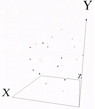
genes (probes). Fig-2 represents the24 breast cancer samples in a 3-D virtual world. Each point in the 3-D space represents a breast cancer sample and was mapped from the original12, 625 dimensional gene expression space. No supervisory information was used to construct the space (i.e. whether a sample is resistant or sensitive), but that information is available through a coloring of the spheres; where black spheres represent sensitive samples, and grey spheres represent resistant. Fig-3 demonstrates another perspective, with the introduction of geometries; where cubes represent resistant samples and spheres represent sensitive samples. It is interesting to notice that there is one resistant sample in between two sensitive samples, and one sensitive sample in between two resistant samples; suggesting that these samples may not have correct class labels.

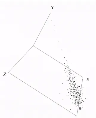
For the other view point (that of viewing similarity between genes) Fig-4 plots361 points in 3-D virtual space. Each point represents a set of points that are mapped to it from the original12, 625 point gene space in 24 dimensions. For example, the large sphere in Fig-4 represents10, 973 very similar (0.95 threshold) genes as measured over the 24 samples provided in the breast cancer data set downloaded. Whereas, the furthest point from that large sphere contains only the single gene31962 at, meaning that it is very different in terms of similarity (when looking at all of the24 samples) from most (as there are a few points near it) of the other12, 625 genes.

Figure 2. Visual representation (3 dimensions) of24 breast cancer samples; each containing 12, 625

genes. Absolute Error= 7.33 · 10−2. Relative Mapping Error= 1.22 · 10−4

6.2

Domain Knowledge Visualization

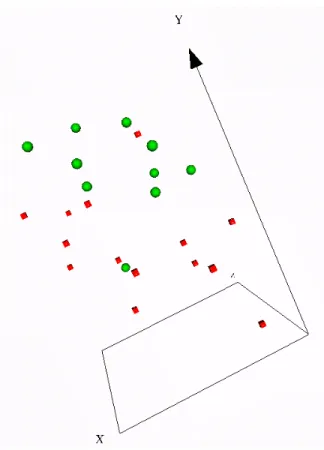
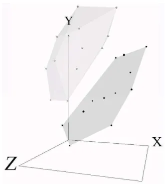
The breast cancer data has domain knowledge embedded in the form of sample classes. In particular, the two classes are sensitive and resistant. In order to more fully understand the class structure based on this domain knowledge, convex hulls can be added to the virtual representation as in Fig-5. The class structures now become much clearer. In particular, the distribution of samples within a class may be observed. For example, the larger resistant class contains samples that seem to be equally spaced throughout the convex hull, while the smaller sensitive class has a markedly different shape, both in terms of size, and distribution. At a more abstract level (that of class structure) the two classes can be observed to touch. When manipulated in the virtual environment (which is difficult to show on printed paper), it becomes clear that one sample from the sensitive class lies just inside that of the resistant classes’ convex hull.

Figure 3. Visual representation (3 dimensions) of24 breast cancer samples; each containing 12, 625

genes. Spheres represent sensitive samples. Cubes represent resistant samples. Absolute Error

= 2.59 · 10−2_{. Relative Mapping Error}= 2.36 · 10−3

6.3

Clustering Results Visualization

Two data mining clustering algorithms were selected in order to generate class information from the breast cancer data. The algorithms were not the subject of this study per se, but rather the results generated by the computational procedures were given to the visualization system in order to investigate the effectivity of the generated visual representations on under-standability. In particular, the visualization system is used as a tool for the explicit demonstration of the clustering results and how those results relate to the underlying data structure. One investigation of the possibility of discovering a subset of genes that may be able to discriminate between the samples better than using the full12, 625 genes (as in this study) is [17].

6.3.1 Forgy’s k-means

Forgy’s k-means algorithm [1] was used to cluster the samples into2 groups, simulating the situation when no class informa-tion is available. That is, the breast cancer sample labels were hidden from the clustering algorithm, forcing the algorithm to perform unsupervised clustering in order to discover the labels based on the data. Fig-6 can be seen to have2 very distinct groups, as requested. Each group has the same number of individuals (12) and both are shaped approximately like ellipsoids. When the virtual world is explored, it is seen that for the upper class, the top sample point is sample GSM4903 (sensi-tive) while the bottom sample point (of the same class) is GSM4918 (resistant), indicating that for this data and algorithm parameters, incorrect classifications were made. Reinforcing the understanding that k-means assumes the data is based on hyperspheres when Euclidean distance is used, which is an assumption that the underlying data structure may not support.

Figure 4. Visual representation (3 dimensions) of12, 625 breast cancer genes from 24 samples. Points

(genes) reduced to 361 via a similarity threshold of 0.95. Large sphere represents 10, 973 genes.

Absolute Error= 9.90 · 10−2. Relative Mapping Error= 1.39 · 10−4

6.3.2 Rough Set k-means

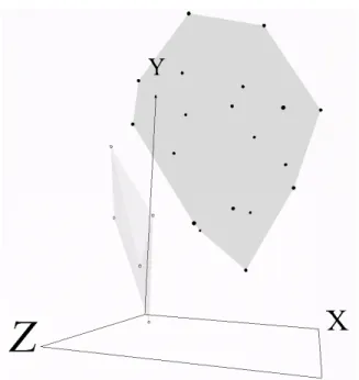
A rough set k-means algorithm [9] was used to cluster the samples into2 groups in a similar fashion as the Forgy’s k-means algorithm. Fig-7 can be seen to have2 classes, as requested. However, one class contains 5 objects and the other class contains the rest. When the small class is investigated, it, like the k-means case above, also does not contain samples from the same (either resistant or sensitive) class. It is interesting, that for this data set, and the particular algorithm parameters (wlower= 0.9, wupper = 0.1, distanceT hreshold = 1) no boundary cases are reported.

6.4

Supervised Visualization

In order to take advantage of the domain knowledge contained within the breast cancer data set in terms of the class infor-mation (resistant, sensitive) a supervised visualization based on nonlinear discriminant analysis (NDA) [18] was performed. All12, 625 genes for each of the 24 samples along with supervisory class information were presented into the multi-layer feedforward neural network and its associated training mechanisms. The purpose was to use the complex neural network training (based on simulated annealing and conjugant gradient) in order to generate a3 dimensional space (the neural net-work used as the mapping function) for the virtual world. The resultant supervised visualization is presented in Fig-8. Each sphere represents a set of breast cancer samples. In particular,5 points are plotted in the visualization, which correspond to the24 samples. The discrepancy occurs because some spheres represent more than one sample. For those multi-sample spheres, the colors presented in the figure, represent the class of the first sample that was placed into that sphere according to the leader clustering algorithm. All spheres except one contain homogeneous information. The exception is the lower right hand sphere, which contains objects9 (GSM4912) and 18 (GSM4914). This exception indicates that the supervised algorithm tried to push the two classes as far apart as possible, but was not able to separate these two objects based on the combination of all12, 625 genes; an extremely high dimensional problem. This may indicate that these two samples are indistinguishable using all12, 625 genes, and that some form of preprocessing would be required (none was performed in this study).

Figure 5. Visual representation (3 dimensions) of24 breast cancer samples with 12, 625 genes. Convex

hulls wrap the resistant(size= 14) and sensitive(size= 10) classes. Absolute Error = 7.33 · 10−2_{. Relative}

Mapping Error= 1.22 · 10−4

Figure 6. Visual representation (3 dimensions) of24 breast cancer samples with 12, 625 genes. Convex

hulls wrap the C1(size= 12) and C2(size= 12) classes discovered by k-means. Absolute Error = 7.06 · 10−2. Relative Mapping Error= 5.21 · 10−5

Figure 7. Visual representation (3 dimensions) of24 breast cancer samples with 12, 625 genes. Convex

hulls wrap the RC1(size= 19) and RC2(size= 5) classes discovered by rough set based k-means.

Absolute Error= 7.06 · 10−2. Relative Mapping Error= 5.21 · 10−5

Figure 8. Supervised Visual representation (3 dimensions) of24 breast cancer samples (5 explicitly

shown) with12, 625 genes as generated by NDA. All spheres are homogeneous except for lower right,

containing one of both sensitive and resistant samples. Sphere colors indicate the class of the first object. Black is resistant; white is sensitive. Absolute Error= 2.999. Relative Mapping Error = 1.44 · 10−9

7

Conclusions

Despite no explicit preprocessing, immersive exploration within 3-D representations of high dimensional data sets fa-cilitates understanding. In particular, some of the visual perspectives presented in this study may be useful for helping to understand breast cancer gene expressions. Visual exploration of the results (when focusing on genes or samples) was very useful for understanding the properties of the computational procedures, in terms of the data and class structures. Further studies focussing on the relationships between particular data mining strategies and visual representations would be interest-ing to pursue.

8

Acknowledgements

This research was conducted within the scope of the BioMine project (National Research Council Canada (NRC), Institute for Information Technology (IIT)). The authors would like to thank Fazel Famili, and Robert Orchard from the Integrated Reasoning Group (NRC-IIT).

References

[1] Anderberg, M.: Cluster Analysis for Applications. Academic Press, (1973) 359pp.

[2] Bazan, J.G., Skowron A., Synak, P: Dynamic Reducts as a Tool for Extracting Laws from Decision Tables. Proc. of the Symp. on Methodologies for Intelligent Systems. Charlotte, NC, Oct. 16-19 1994. Lecture Notes in Artificial Intelligence 869, Springer-Verlag (1994), 346–355.

[3] Borg, I., and Lingoes, J., Multidimensional similarity structure analysis: Springer-Verlag, New York, NY (1987), 390 p. [4] Chandon, J.L., and Pinson, S., Analyse typologique. Thorie et applications: Masson, Paris (1981), 254 p.

[5] Chang, J.C. et al. “Gene expression profiling for the prediction of therapeutic response to docetaxel in patients with breast cancer”. Mechanisms of Disease. THELANCET. vol 362. August 2003.

[6] Gower, J.C., A general coefficient of similarity and some of its properties: Biometrics, v.1, no. 27, p. 857–871. (1973). [7] Hartigan, J.: Clustering Algorithms. John Wiley & Sons, 351 pp, (1975).

[8] A. K. Jain and J. Mao , “Artificial Neural Networks for Nonlinear Projection of Multivariate Data,” Proceedings of the 1992 IEEE joint Conf. on Neural Networks, Baltimore, MD, June. 1992, pp. 335–340.

[9] Lingras, P., and Yao, Y. “ Time Complexity of Rough Clustering: GAs versus K-Means.” Third. Int. Conf. on Rough Sets and Current Trends in ComputingRSCTC 2002. Malvern, PA, USA, Oct 14-17. Alpigini, Peters, Skowron, Zhong (Eds.) Lecture Notes in Computer Science (Lecture Notes in Artificial Intelligence Series) LNCS 2475, pp. 279-288. Springer-Verlag, 2002.

[10] J. Mao and A. K. Jain, “Discriminant Analysis Neural Networks,” Proceedings of the 1993 IEEE International Confer-ence on Neural Networks, San Francisco, California, Mar. 1993, pp. 300–305.

[11] J. Mao and A. K. Jain, “Artificial Neural Networks for Feature Extraction and Multivariate Data Projection,” IEEE Trans. on Neural Networksvol. 6, pp. 296–317, Mar. 1995.

[12] T. Masters, Advanced Algorithms for Neural Networks, John Wiley & Sons, 1993.

[13] Pawlak, Z., Rough sets: Theoretical aspects of reasoning about data: Kluwer Academic Publishers, Dordrecht, Nether-lands, 229 p. (1991).

[14] J. J. Vald´es, “Virtual Reality Representation of Relational Systems and Decision Rules: An exploratory Tool for under-standing Data Structure,” In Theory and Application of Relational Structures as Knowledge Instruments, Meeting of the COST Action 274 (P. Hajek. Ed), Prague, Nov. 2002.

[15] J. J. Vald´es, “Similarity-Based Heterogeneous Neurons in the Context of General Observational Models,” Neural Net-work Worldvol. 12, no. 5, pp. 499–508, 2002.

[16] J. J. Vald´es, “Virtual Reality Representation of Information Systems and Decision Rules: An Exploratory Tool for Understanding Data and Knowledge,” Lecture Notes in Artificial Intelligence LNAI 2639, Springer-Verlag, 2003, pp. 615– 618.

[17] J. J. Vald´es and A. J. Barton. “Gene Discovery in Leukemia Revisited: A Computational Intelligence Perspective”, Proceedings of the 17th International Conference on Industrial and Engineering Applications of Artificial Intelligence and Expert Systems, Lecture Notes in Artificial Intelligence LNAI 3029, Springer Verlag, 2004, pp. 118–127.

[18] J. J. Vald´es and A. J. Barton. “Virtual Reality Visual Data Mining with Nonlinear Discriminant Neural Networks: Application to Alzheimer and Leukemia Gene Expression Data”, Proceedings of the International Joint Conference on Neural Networks 2005, Lecture Notes in Artificial Intelligence, Springer Verlag, 2005, To appear.

[19] A. R. Webb and D. Lowe, “The Optimized Internal representation of a Multilayer Classifier”, Neural Networks vol. 3, pp. 367-375, 1990.

[20] Wr´oblewski, J: Ensembles of Classifiers Based on Approximate Reducts. Fundamenta Informaticae 47 IOS Press, (2001), 351–360.