Dynamique climatique de l'océan Pacifique ouest équatorial au cours du Pléistocène récent

HAL Id: tel-00008934

https://tel.archives-ouvertes.fr/tel-00008934

HAL is a multi-disciplinary open access archive for the deposit and dissemination of sci-entific research documents, whether they are pub-lished or not. The documents may come from teaching and research institutions in France or abroad, or from public or private research centers.

L’archive ouverte pluridisciplinaire HAL, est destinée au dépôt et à la diffusion de documents scientifiques de niveau recherche, publiés ou non, émanant des établissements d’enseignement et de recherche français ou étrangers, des laboratoires publics ou privés.

Dynamique climatique de l’océan Pacifique ouest

équatorial au cours du Pléistocène récent

Thibault de Garidel-Thoron

To cite this version:

Thibault de Garidel-Thoron. Dynamique climatique de l’océan Pacifique ouest équatorial au cours du Pléistocène récent. Géologie appliquée. Université de droit, d’économie et des sciences - Aix-Marseille III, 2002. Français. �tel-00008934�

UNIVERSITE DE DROIT, D'ECONOMIE ET DES SCIENCES D'AIX-MARSEILLE (AIX-MARSEILLE III)

ECOLE DOCTORALE SCIENCES DE L’ENVIRONNEMENT

N° attribué par la bibliothèque

|__|__|__|__|__|__|__|__|__|__|

T H E S E

pour obtenir le grade de

DOCTEUR DE L'UNIVERSITE DE DROIT, D’ECONOMIE ET DES SCIENCES D’AIX-MARSEILLE

(AIX-MARSEILLE III)

Discipline : Géosciences de l’Environnement

présentée et soutenue publiquement

par

Thibault de GARIDEL-THORON

Le 19 juillet 2002

Titre :

DYNAMIQUE CLIMATIQUE DE L’OCEAN PACIFIQUE OUEST EQUATORIAL AU COURS DU PLEISTOCENE RECENT

_______

Directeur de thèse :

M. Luc BEAUFORT ______

JURY

M. Edouard BARD, Professeur, Collège de France Co-directeur M. Luc BEAUFORT, Chargé de Recherche CNRS, Aix-en-Provence Directeur de thèse Mme. Elsa CORTIJO, Chargée de Recherche CNRS, Gif-sur-Yvette Examinateur M. Patrick DE DECKKER, Professeur, Australian National University Rapporteur M. Dick KROON, Professeur, Vrije Universteit Amsterdam, Rapporteur M. Nicolas THOUVENY, Professeur, Université de la Méditerranée Examinateur

Remerciements :

Je remercie Luc Beaufort de la confiance et de la liberté qu’il m’a accordé au cours de ces quatre dernières années pour mes travaux de recherche. Je voudrais lui témoigner du plaisir que j’ai eu à travailler avec lui, du Marion-Dufresne au CEREGE et lui exprimer toute ma reconnaissance pour son aide enthousiaste.

Je remercie Mme Elsa Cortijo, MM. Edouard Bard, Dick Kroon, Patrick De Deckker, et Nicolas Thouveny d’avoir accepté de participer à l’évaluation de ce travail.

Je remercie parmi les personnes avec qui j’ai eu le plaisir de travailler, Edith Vincent qui m’a fait découvrir la taxonomie des foraminifères planctoniques, Franck Bassinot pour sa vision du monde de la géochimie isotopique, Edouard Bard et sa connaissance indéfectible de la paléocéanographie, Brad Linsley, Alan Mix, Lucas Lourens, Nicolas Thouveny et enfin Patrick De Deckker qui m’a ouvert la piste des Orbulines et m’a permis d’utiliser des données non publiées.

Merci à Philippe Dussouillez pour son travail sur SYRACO qui a permis de rendre opérationnel le système d’acquisition automatique d’images sur la loupe binoculaire.

L’aboutissement (?) de ce travail correspond à la fin d’un séjour de plus de quatre années passées au sein du CEREGE. Je remercie en premier lieu Noelle Buchet de m’avoir supporté dans son bureau sans jamais ciller sur le désordre entourant mon bureau et colonisant le sien progressivement. Merci également à tous les jeunes “étudiants-chercheurs”, de l’ancienne génération à la nouvelle croisés au désormais célèbre “chez Brigitte”, Olivia, Denis, Delphine, Corinne, Ouassila, Eva, Claire, Gilles, Doriane future partenaire de la French Connection à Rutgers, Yannick, Florian, Anne, Doris, Sarah, Jérôme (le catalan), Julien, Martine, Bruno, Christophe et ceux que j’oublie...

Je voudrais remercier en particulier Yannick pour son soutien amical, particulièrement précieux pendant ces derniers mois, et lui exprimer toute mon amitié.

Car il y a de la vie en dehors de l’Arbois, et plus certainement que sur les météorites martiennes chères à Jérôme et Maria, merci aux extra-CEREGE, Guillemette, Estelle et spécialement Camille rencontrées en mer ou dans les montagnes, dont les conversations scientifiques (ou pas) ont contribué plus ou moins directement à ce manuscrit.

J’exprime ma reconnaissance aux jeunes maîtres de conférences, Yann, Laurence, Pierre-Etienne ainsi qu’aux autres demi-hatères Yannick et Jérôme, qui m’ont aidé dans le montage de mes enseignements et m’ont fait gagner un temps précieux pour la rédaction.

Un grand merci également à mes deux familles, ma famille pour son soutien constant, et ma famille “adoptive”, chez qui tout est plus simple.

Et bon courage aux futurs docteurs qui ne liront de cette thèse que les remerciements… Un dernier et ultime merci à Marion.

The end.

Cette thèse a été financée grâce à une allocation du Ministère de la Recherche, et par un contrat d’ATER à l’université d’Aix-Marseille III.

TABLE DES MATIERES

Introduction………..………...5

A – Introduction Générale………5

B – Structure de la thèse……….………11

Dynamique Climatique rapide Chapitre 1 : Variabilité millénnale de la mousson d’hiver Est-Asiatique :………15

Problématique Méthode………..15

Résumé de l’article……….17

Millenial-scale dynamics of the East asian winter monsoon during the last 200,000 years : de Garidel-Thoron, T., Beaufort, L., Linsley, B., and Dannennmann, S. (2001) Paleoceanography, v. 16, p. 491-508 Abstract………..19 1. Introduction……….19 2. Material………...21 3. Methods………...22 3.1 Age model 3.2 Signal Analysis 3.2.1. Spectral Analysis 3.2.2. Singular Spectrum Analysis 3.3 Florisphaera profunda : paleoproductivity marker 4. Results……….25

4.1 Glacial-interglacial variations 4.2 Sub-Milankovitch dynamics 4.2.1 Bolling/Allerod and the Younger Dryas event 4.2.2 Millennial-scale PP events during MIS 3 4.3 Analysis in the Frequency Domain (Suborbital Frequencies) 4.3.1 The 1.5 kyr cycle 4.3.2 The 2.4 kyr cycle 4.3.3 The 4.2-3.3 kyr cycle 4.3.4 The 6 kyr cycle 5. Discussion: High-Frequency Cycles………...32

5.1 The 2.4 kyr Cycle 5.2 Pseudo 1.5 kyr Cyclicity 6. Conclusions……….34

References………..35

Chapitre 2 : Relargages massifs de clathrates de méthane pendant le dernier stade glaciaire :……….39

Problématique Méthodes……….42

Résumé de l’article……….43 Références

Large gas hydrate methane releases during the last glacial stage. de Garidel-Thoron, T., Beaufort, L. and Bassinot F. soumis à Geology.

Abstract………..45

Introduction………45

Material and Method………..46

Results……….47

Discussion………...49

References………...53

Dynamique glaciaire-interglaciaire Chapitre 3 : Température des eaux de surface du Pacifique Ouest équatorial :……….57

Problématique Principe des fonctions de transfert………..58

1- Les fonctions de transfert d’Imbrie et Kipp 2- La méthode des analogues 3- Les réseaux neuronaux Résumé de l’article……….59

Glacial-interglacial sea-surface temperature changes in the Western Pacific warm pool inferred from planktonic foraminifera and alkenones. de Garidel-Thoron, T., Beaufort, L., Bard, E., Sonzogni, C., and Mix, A.C., : soumis à Paleoceanography. Abstract………...61

1. Introduction………..62

2. Methods………..………..62

2.1.1. Imbrie-Kipp transfer functions 2.1.2. Modern Analog Technique (MAT) 2.1.3. A regional transfer function for the Western Pacific 2.1.3.1.1. Core-top data-set 2.1.3.1.2. Oceanic parameters 2.1.4. Downcore analysis : foraminifera and stratigraphy 2.1.5. Alkenone measurements 3. Results………..67

3.1.1. Eastern equatorial Pacific an anomalous area ? - modification of the core-top data-set 3.1.2. Faunal factors 3.1.3. Evaluating transfer function bias 3.1.4. Application to the Western Pacific core MD 97-2138 3.1.5. Alkenones SSTs 4. Discussion : The glacial SSTs in the Western Pacific……….76

4.1.1. The last glacial maximum 4.1.2. Precession and ENSO dynamics in the Western Equatorial Pacific 4.1.3. The marine isotope stage 6 5. Conclusions……….….………81

References……….……….82

Chapitre 4 : Forçage « ENSO-like » de la productivité primaire du Pacifique Ouest pendant le Pléistocène récent………..87

Problématique Résumé de l’article……….88

ENSO-like forcing on oceanic primary production during the late Pleistocene (2001) - Beaufort, L., de Garidel-Thoron, T., Mix, A.C., and Pisias, N.G. Science, v. 293, p. 2440-2444. Abstract………...89

Manuscript………..89

Supplemental data :……….97

Counting methods………..……….98

Figures………99

References………..99

Morphométrie des foraminifères et paléocéanographie Chapitre 5 : Orbulina universa : morphométrie et paramètres environnementaux dans le Pacifique ouest………..101

Problématique Résumé………..102

Morphometry of Orbulina universa in the Western Pacific ocean, manuscrit en préparation Abstract……….103

1. Introduction………104

2. Methodology………..105

2.1. Optic microscopy 2.2. S.E.M. images : porosity of the test 2.3. Sediment samples 2.4. Oceanic parameters 2.5. Oceanic and climatological setting 3. Results………109

3.1. Modern calibration 3.1.1. Size distribution of inner porosity 3.1.2. Size distribution of external porosity 3.1.3. Modern calibration of the inner porosity 3.1.4. Porosity and mean diameter 3.1.5. Modern calibration of the test size 3.2. Downcore application 3.2.1. Inner porosity 3.2.2. Diameter 3.2.2.1. Orbital scale oscillations : application to the MD97-2138 core 3.2.2.2. Millenial-scale variability : application to the MD97-2134 core 4. Discussion………..119

4.1.1. Geographic distribution of the different types of O. universa 4.1.2. Morphometry and potential cryptic species of O. universa 4.1.3. Factors affecting the mean size of Orbulina 4.1.4. Sea-surface density inferred from O. universa 5. Conclusions………123

References……….124

Chapitre 6 : Reconnaissance automatique des foraminifères planctoniques : étude préliminaire Introduction………..127

Matériels et Méthodes………..128

Système d’acquisition automatique des images de foraminifères Réseau de neurones Base de données images d’apprentissage Fonctionnement de SYRACO Résultats………132

Tests sur une base de données Tests sur des images réelles Discussion………137

Conclusions………...139

Références……….140

Conclusions et perspectives………141

Annexe : Continental biomass burning and oceanic primary production estimates in the Sulu sea record East Asian summer and winter monsoon for the last 380 kyrs: Marine Geology.(accepté) - Beaufort, L., de Garidel-Thoron, T., Linsley, B., Oppo, D., and Buchet, N. Abstract……….145 1. Introduction………146 2. Material………..148 3. Methods………..148 3.1. Microscopic charcoals 3.2. Coccoliths 3.3. Counting 3.4. Primary Production transfer function 3.5. Chronostratigraphy 3.6. Time-series analysis 4. Results………152

5. Discussion………..154

5.1. Winter monsoon dynamics 5.2. Biomass Burning 5.2.1. Human impact 5.2.2. Summer monsoon 5.3. Relation between summer and winter monsoons 6. Conclusions………158

Introduction :

L’augmentation des températures moyennes de l’hémisphère nord au cours du 20eme siècle a posé la question de la séparation de la variabilité climatique naturelle de celle liée à l’action anthropique. Pour pouvoir déconvoluer l’action humaine, il est nécessaire de décrire et de quantifier les variations climatiques naturelles qui ont affectées le climat terrestre, et d’estimer la part relative des mécanismes associés à ces variations. Ce travail de thèse s’inscrit dans cette vaste problématique de description et de quantification de la variabilité naturelle du climat.

A. Introduction Générale

Au cours des deux derniers millions d’années, la Terre a connu une succession de longues périodes glaciaires pendant lesquelles les hautes latitudes étaient recouvertes de glace, alternant avec de courtes périodes interglaciaires dont font partie les 10 000 dernières années (Holocène). Cette succession de périodes glaciaires et interglaciaires a suivi des périodicités d’environ 100 000 ans au cours des derniers 800 000 ans. Des changements de périodes de 41 000 et environ 21 000 ans marquent également les enregistrements paléoclimatiques. Ces changements climatiques ont été liés aux modifications périodiques de la distribution de l’insolation créées par les oscillations orbitales de la terre, appelées cycles de Milankovitch qui possèdent les mêmes caractéristiques spectrales. Ainsi, le cycle de 100 000 ans correspond-il aux variations de l’excentricité de l’orbite de la terre autour du soleil, le cycle de 41 000 ans à l’obliquité de l’axe de rotation de notre planète et le cycle d’environ 21 000 ans à la précession des équinoxes. Ces deux derniers paramètres influencent la distribution spatiale et saisonnière de l’insolation, alors que l’excentricité module la quantité absolue d’énergie solaire reçue. Depuis la formulation de cette théorie par Milankovitch, et sa confirmation par les travaux des 30 dernières années subsiste la question de l’intervention de fortes boucles de rétroactions positives dans le système climatique, indispensables à l’amplification des faibles variations d’insolation.

Les enregistrements climatiques des carottes de glace polaires ont montré que les variations de concentration en CO2 atmosphérique suivent ces cycles glaciaires-interglaciaires, variations comprises par exemple entre 280 ppm pour l’Holocène et 180 à 200 ppm pour le dernier maximum glaciaire, il y a environ 21 000 ans (Petit et al., 1999). Le CO2 étant un gaz à effet de serre, des travaux de modélisation ont permis de mettre en évidence son rôle important dans les changements climatiques à l’échelle glaciaire-interglaciaires. Outre des processus uniquement liés aux modifications physico-chimiques de l’océan, de telles variations du cycle du carbone impliquent (a) l’extraction de carbone de l’océan de surface par l’action de la pompe biologique qui va fixer sous forme de calcite le CO2

Introduction

dissous dans la colonne d’eau, et (b) des changements associés dans le budget des carbonates de calcium marins. Dans l’état actuel des connaissances, les pompes biologiques des basses et hautes latitudes ont toutes deux joué un rôle dans ce piégeage du CO2 (Sigman and Boyle, 2000).

Aux basses latitudes, les sédiments carbonatés attestent du fonctionnement de la pompe biologique au cours du temps. En effet, ces sédiments sont majoritairement constitués de coccolithes et de tests de foraminifères planctoniques. Les coccolithophoridés qui sécrètent les plaques de calcite microscopiques (environ 5 µm) appelées coccolithes sont des organismes phytoplanctoniques, alors que les foraminifères planctoniques (200 à 500 µm environ) font partie du zooplancton. L’étude de ces organismes va permettre de reconstituer au cours du temps les changements d’activité de la pompe biologique. Comme ces organismes vivent dans la zone de mélange océanique, qui est influencée par les conditions atmosphériques de surface, leurs microfossiles vont également être des témoins des conditions paléoclimatiques.

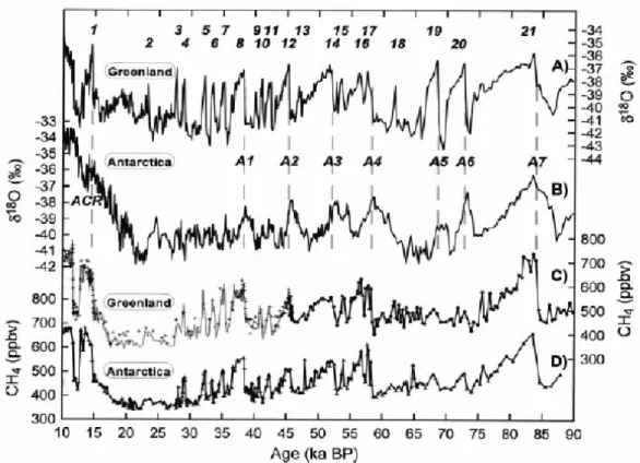
Figure 1 : événements de Dansgaard/Oeschger révélés par les isotopes de l’oxygène dans la carotte de glace GRIP du Groenland (numérotés de 1 à 21). En comparaison figurent les variations observées dans l’Antarctique, et les variations de concentration en méthane atmosphérique (d’après (Blunier and Brook, 2001))

Depuis une dizaine d’années, un nouveau champ de recherches s’est ouvert avec les études paléoclimatiques à haute résolution. Ainsi, l’analyse à haute résolution des isotopes de l’oxygène dans les carottes de glace du Groenland, a permis de mettre en évidence des changements abrupts du climat pendant les 60 000 dernières années (Dansgaard et al., 1993). Ces changements abrupts, les événements de Dansgaard/Oeschger, débutent par un réchauffement abrupt des températures atmosphériques au Groenland de 5-10°C en quelques décennies ou moins, et sont suivis par un

refroidissement graduel sur quelques centaines ou milliers d’années (figure 1.). Le refroidissement accélère pour atteindre la phase la plus froide du cycle (stadiaire). Ces oscillations de température sont également associées à des changements significatifs de la concentration atmosphérique en gaz à effets de serre (le CH4 par exemple), qui ont sans doute joué un rôle d’amplificateur comme au cours des cycles glaciaire/interglaciaires (Alley et al., 1999). La durée moyenne d’un cycle est d’environ 1500 ans. L’étude des carottes sédimentaires de l’Atlantique Nord montre que ces changements de température sont à mettre en relation avec des modifications de la circulation océanique.

Dans l’Atlantique Nord, le réchauffement différentiel des basses latitudes par rapport aux hautes latitudes tend à accélérer la circulation des eaux de surface vers les pôles, alors que l’évaporation aux basses latitudes, et l’apport d’eaux peu salées aux hautes latitudes tendent inversement à réduire cette circulation. Actuellement, le gradient thermique joue un rôle plus critique que celui du gradient de salinité des eaux de surface. Ainsi, le flux d’eaux de surface chaudes chaudes vers le Nord est contrebalancé par la formation des eaux profondes Nord-Atlantique dans les mers Nordiques qui plongent vers le Sud. Il n’existe pas dans les autres océans de similaires zones de convection. Les eaux profondes Nord-Atlantique vont donc alimenter une boucle de circulation océanique globale, la circulation thermohaline (figure 2).

Figure 2 : Schéma de la circulation thermohaline globale (d’après Broecker, 1998)

L’analyse des carottes sédimentaires de l’Atlantique Nord a permis de mettre en évidence l’existence de trois différents régimes de la circulation thermohaline caractérisés par des intensités spécifiques de formation d’eaux profondes et par la localisation des zones de convection

Introduction

océaniques(Alley et al., 1999). Ces changements d’intensité de la circulation thermohaline sont associés aux événements climatiques de Dansgaard/Oeschger. Schématiquement, les périodes de réchauffement rapide culminant à des températures comparables à celles modernes – les interstadiaires, correspondent à une reprise de la circulation thermohaline, qui suivent des périodes froides pendant lesquelles la circulation thermohaline était plus ou moins ralentie. En particulier, celle-ci était très fortement réduite lors des événements de Heinrich, gigantesques débâcles d’icebergs dans l’Atlantique Nord qui ponctuent certains stadiaires du dernier stade glaciaire.

La variabilité climatique Dansgaard/Oeschger détectée pour la première fois dans les régions circum-Atlantique n’est pas spécifique à cette zone. Les variations de concentration en méthane atmosphérique des carottes de glaces polaires, supportent l’idée d’une dynamique similaire du cycle hydrologique aux basses latitudes, la source principale du méthane étant les zones humides des basses latitudes(Chappellaz et al., 1993). De nombreux enregistrements montrent que les événements de D/O ont été présents aux basses latitudes, même si le phasage précis est encore incertain. Par exemple des enregistrements de mousson indienne sur la marge Pakistanaise (Schulz et al., 1998), d’oxygénation dans le bassin de Santa Barbara(Behl and Kennet, 1996), tous deux à des basses latitudes, montrent également une dynamique de type D/O.

Le cycle hydrologique aux basses latitudes est donc une des questions majeures concernant la variabilité climatique, que ce soit à l’échelle glaciaire-interglaciaire, ou que ce soit pour les événements de type D/O . En effet, la vapeur d’eau est le principal gaz à effet de serre, et peut donc jouer un rôle d’amplificateur dans le système climatique, tout comme le CO2 et le CH4. De plus la circulation thermohaline, dont les variations sont reconnues comme ayant un impact global aux échelles de temps glaciaire-interglaciaire et millénnales, est fondamentalement influencée par les gradients de salinité entre les basses latitudes et les hautes.

A l’échelle interannuelle par exemple, des travaux récents ont mis en évidence le lien entre l’intensité de la circulation thermohaline et la distribution spatiale des températures de surface de l’océan Pacifique équatorial. Tout comme de larges débâcles d’icebergs influent la dynamique de la circulation thermohaline, des modifications des quantités d’eau douce transférées entre le Pacifique et l’Atlantique modulent l’intensité de la convection dans l’océan Atlantique Nord (Schmittner et al., 2000) Cette influence du système couplé océan-atmosphère des basses latitudes, a été également démontrée à l’échelle glaciaire-interglaciaire (Schmittner and Clement, 2002).

Le rôle des tropiques est donc fondamental dans la circulation océanique globale, et en particulier la circulation thermohaline. La zone intertropicale étant celle recevant le plus d’énergie solaire, elle est également à l’origine des grands processus atmosphériques. A l’échelle saisonnière, les systèmes de mousson permettent de transférer de très grandes quantités d’énergie d’un hémisphère à l’autre ; que ce soit dans l’océan Indien avec la mousson Indienne, ou que ce soit dans l’océan

Pacifique avec la mousson Est-Asiatique. A l’échelle interannuelle, le phénomène d’El Nino-Oscillation Australe (désigné par l’acronyme ENSO, d’ « El Nino-Southern Nino-Oscillation ») est la première cause de variabilité climatique globale par le biais des téléconnexions. Ces deux phénomènes prennent leur source dans la zone d’eaux chaudes du Pacifique ouest équatorial (en anglais, « Western Pacific Warm Pool ») qui avec des eaux de surface toujours plus chaudes que 28°C constitue le centre de convection le plus actif de l’atmosphère du globe.

HIVER HN

ETE HN

mousson

transverse

mousson

transverse

> 27

°C

mousson

latérale

mousson

latérale

figure 3 : cellules de circulations atmosphériques (d’après Webster, 1998)

Le maintien des températures de surface très chaudes dans le Pacifique ouest est lié à la cellule de Walker zonale (1) qui par la tension des alizés sur les eaux de surface de l’océan Pacifique équatorial empile sur la marge occidentale une lentille d’eau chaude. Cette structure est marqué par un gradient des températures de surface entre le Pacifique ouest et la marge américaine, accompagné d’une pente de la thermocline, la thermocline étant plus profonde dans l’ouest Pacifique. Périodiquement, tous les 3 à 6 ans actuellement, cette structure zonale est perturbée lors des

Introduction

événements de El Nino. Le centre de convection est déplacé vers l’Est Pacifique, alors que les alizés sont affaiblis, une anomalie positive de température se propage vers l’Est le long de l’équateur. La pente de la thermocline le long de l’équateur est également modifiée, avec un approfondissement significatif vers les marges américaines, et une remontée dans l’Ouest Pacifique.

Deux autres systèmes de circulation atmosphériques sont liés à l’existence de cette zone d’eaux chaudes (Webster et al., 1998). (2) La seconde cellule atmosphérique est méridionale, et correspond au phénomène saisonnier de mousson Asiatique. Cette cellule de mousson latérale, est très active dans le Pacifique ouest pendant l’hiver boréal (mousson d’hiver Est-asiatique). (3) Une troisième cellule transverse relie l’Afrique de l’Ouest à l’archipel Indonésien. Cette cellule constitue un dipôle comparable à la circulation de Walker de l’océan Pacifique, mais elle est également fortement influencée par l’orographie (plateau Tibétain) et la migration de la zone de convergence intertropicale (Saji et al., 1999).

Si le Pacifique équatorial occidental fait l’objet de nombreuses études sur la dynamique climatique actuelle, la variabilité paléoclimatique reste peu étudiée et très discutée. La première raison de la relative absence de travaux sur cette zone, tient à la rareté des enregistrements sédimentaires possédant un taux de sédimentation adapté aux études des derniers cycles climatiques. Cette rareté des enregistrements est elle-même lié à la configuration bathymétrique du Pacifique ouest, la plus grande partie des fonds océaniques étant à une profondeur plus grande que celle de préservation des carbonates. Les meilleurs enregistrements disponibles jusqu’à présents ne possédaient pas de taux de sédimentation suffisants pour offrir une résolution permettant de s’affranchir de l’effet de lissage de la bioturbation. Une deuxième raison des grandes discussions concernant le Pacifique ouest, est liée aux conditions environnementales exceptionnellement chaudes qui sont rarement prises en compte dans les gammes de calibrations des marqueurs (« proxies ») environnementaux.

Les carottes sédimentaires prélevées au cours de la campagne océanographique IMAGES III-IPHIS du Marion-Dufresne dans l’océan Pacifique occidental équatorial (figure 4) nous ont permis d’étudier avec des taux de sédimentation uniques la variabilité paléoclimatique de cette zone. L’abondance en microfossiles carbonatés dans ces sédiments en font des outils adaptés pour tracer la dynamique des eaux superficielles du Pacifique équatorial occidental au cours du Pléistocène récent. Cette thèse décrit la variabilité climatique de cette zone, de l’échelle millénnale à celle des cycles orbitaux.

100°E 100°E 120°E 120°E 140°E 140°E 160°E 160° E 180°E 180°E 20°S 20°S 0° 0° 20°N 20°N MD97-2134 MD97-2141 MD97-2138 Océan Pacifique Océan Indien MD97-2140 Mer de Chin e Mér idio nale Mer de Sulu

Figure 4 : carte de localisation des carottes étudiées

B. Structure de cette thèse

Formellement, la plus grande partie des résultats obtenus pendant cette thèse ont fait l’objet de rédaction d’articles en anglais. J’ai fait le choix de conserver les articles originaux, en introduisant brièvement chaque article par un exposé de la problématique scientifique, en détaillant les méthodes utilisées dans chaque article, et en résumant les principaux résultats. Les chapitres ont été classés dans trois parties dont la séparation est nécessairement arbitraire, et ne permet pas de s’affranchir des recoupements entre ces différentes parties. La première partie concerne les changements climatiques à l’échelle millénnale du climat dans le Pacifique Ouest. La seconde partie se concentre sur les changements à l’échelle glaciaire-interglaciaire. Et enfin, la dernière partie traite plus spécifiquement des méthodologies concernant les foraminifères planctoniques.

I - Dynamique paléoclimatique rapide :

Le premier chapitre décrit un enregistrement à haute résolution de la Production Primaire en mer de Sulu, un marqueur de la dynamique de la mousson d’hiver. Dans ce chapitre, nous discutons des problèmes de téléconnexions entre la mousson Est-asiatique et les hautes latitudes pour les événements de Dansgaard-Oeschger. Nous nous sommes également attaché à décrire finement les caractéristiques spectrales de cet enregistrement, pour tester la stabilité dans le temps des fréquences suborbitales.

Introduction

Le deuxième chapitre concernant les changements climatiques rapides décrit un enregistrement à très haute résolution de l’hydrologie de surface du Golfe Papou. Nous montrons que de brusques relargages de méthane se sont produits pendant le dernier stade glaciaire l.s. dans la mer de Corail. Ces relargages sont interprétés comme étant liés à la dissociation thermique de gaz hydrates de méthane pendant les bas niveaux marins. Ces relargages peuvent avoir un effet de rétroaction positive important pour le climat global.

II - Dynamique glaciaire/interglaciaire

Le premier chapitre décrit un nouvel enregistrement des températures des eaux de surface dans le cœur du réservoir d’eau chaude du Pacifique Ouest, qui remet en accord les valeurs de températures estimées par les données issues des comptages de foraminifères planctoniques de celles estimées par les alkénones. Une nouvelle fonction de transfert évitant des biais liés selon nous à la structure des écosystèmes a été développée pour toute la bande équatoriale sauf le Pacifique Est. Cet enregistrement confirme les estimations de température au dernier maximum glaciaire de CLIMAP.

Le deuxième chapitre décrit une série d’enregistrements de production primaire le long de l’équateur dans les océans Indo-Pacifiques. La profondeur de la thermocline le long de l’équateur apparaît suivre un balancement entre le Pacifique équatorial occidental d’une part, et le Pacifique Est et l’Ouest de l’océan Indien d’autre part, à l ‘échelle de la précession. Ce mécanisme est analogue à celui de l’ENSO, et de la cellule de circulation atmosphérique de la mousson indienne qui actuellement sont présents à l’échelle interannuelle. L’existence d’un cycle à 30 000 ans dans ces enregistrements, similaire à celui observé dans les variations de concentration atmosphériques en CO2, souligne le rôle de la pompe biologique aux basses latitudes.

III – Morphométrie des foraminifères planctoniques :

L’étude du génotype de foraminifères planctoniques a mis en évidence une diversité cryptique insoupçonnée auparavant. Celle-ci nécessite un effort de caractérisation morphométrique. Ce premier chapitre prend l’exemple d’Orbulina universa dans le Pacifique ouest. En utilisant les critères de porosité et de taille moyenne du test de ce foraminifère nous caractérisons la diversité morphologique de cette espèce. La calibration des ces deux critères en fonction de divers paramètres environnementaux a été ensuite testée dans deux enregistrements sédimentaires du Pacifique ouest.

La reconnaissance automatique des foraminifères qui permettrait d’étudier en routine la morphométrie des foraminifères, et donc de tester de nouvelles fonctions de transfert basées sur une taxonomie quantitative a fait l’objet d’une étude préliminaire. La méthode des réseaux de neurones a été appliquée avec succès au nannoplancton. Nous montrons dans ce chapitre les résultats préliminaires de cette méthodologie adaptée aux foraminifères planctoniques.

Références :

Alley, R.B., Clark, P.U., Keigwin, L.D., and R.S., W., 1999, Making sense of millennial-scale climate change, Mechanisms of global climate change at millennial time scales, Volume 112: Geophysical Monograph, American Geophysical Union, p. 385-394.

Behl, R., and Kennet, J.P., 1996, Brief interstadial events in the Santa Barbara basin, NE Pacific, during the past 60 kyr: Nature, v. 379, p. 243-246.

Blunier, T., and Brook, E.J., 2001, Timing of millenial-scale climate change in Antarctica and Greenland during the last glacial period: Science, v. 291, p. 109-112.

Chappellaz, J., Blunier, T., Raynaud, D., Barnola, J.-M., Schwander, J., and Stauffer, B., 1993, Synchronous changes in atmospheric methane and Greenland climate between 40 and 8 kyBP: Nature, v. 366, p. 443-445.

Dansgaard, W., Johnsen, S.J., Clausen, H.B., Dahl-Jensen, D., Gundestrup, N.S., Hammer, C.U., Hvidberg, C.S., Steffensen, J.P., Sveinbjörnsdottir, A.E., Jouzel, J., and Bond, G., 1993, Evidence for general instability of past climate from a 250 kyr ice-core record: Nature, v. 364, p. 218-220.

Petit, J.R., Jouzel, J., Raynaud, D., Barkov, N.I., Barnola, J.-M., Basile, I., Bender, M., Chappelaz, J., Davis, M., Delaygue, G., Delmotte, M., Kotlyakov, V., Legrand, M., Lypenkov, V.Y., Lorius, C., Pépin, L., Ritz, C., Saltzman, E., and Stievenard, M., 1999, Climate and atmospheric history of the past 420,000 years from the Vostok ice-core, Antartica: Nature, v. 399, p. 429-436.

Saji, N.H., Goswani, B.N., Vinayachandran, P.N., and Yamagata, T., 1999, A dipole mode in the Indian Ocean: Nature, v. 401, p. 360-362.

Schmittner, A., Appenzeller, C., and Stocker, T., 2000, Enhanced Atlantic freshwater export during El Niño: Geophysical Research Letters, v. 27, p. 1163-1166.

Schmittner, A., and Clement, A.C., 2002, Sensitivity of the thermohaline circulation to tropical and high latitude freshwater forcing during the last glacial-interglacial cycle: Paleoceanography, v. 17, p. 10.1029/2000PA000591.

Schulz, H., von Rad, U., and Erlenkeuser, H., 1998, Correlation between Arabian Sea and Greenland climate oscillations of the past 110,000 years: Nature, v. 393, p. 54-57.

Sigman, D.M., and Boyle, E.A., 2000, Glacial/interglacial variations in atmospheric carbon dioxide: Nature, v. 407, p. 859-869.

Webster, P.J., Magaña, V.O., Palmer, T.N., Shukla, J., Tomas, R.A., Yanai, M., and Yasunari, T., 1998, Monsoons: processes, predictability, and the propects for prediction: Journal of Geophysical Research, v. 103, p. 14451-14510.

Partie I

-Dynamique Climatique

Rapide

Chapitre 1 : Variabilité millénnale de la mousson d’hiver Est-Asiatique

Même si les variations rapides du climat étaient suspectées depuis les années 1970 (e.g. (Pisias et al., 1973)), l’analyse à haute résolution des carottes de glace a révélé l’existence de variations abruptes du climat au cours des 60000 dernières années dans les régions circum-Atlantique (Dansgaard et al., 1993). Ces variations abruptes ont également été décelées dans des enregistrements de basses latitudes, par exemple dans des enregistrements de température dans l’océan Atlantique Nord (Sachs and Lehman, 1999). Des événements similaires ont également été mis en évidence dans enregistrements sédimentaires d’intensité de la mousson indienne (Schulz et al., 1998) ; ou dans le Pacifique Est (Behl and Kennet, 1996). La dynamique de la zone Est-asiatique à l’échelle millénnale restait mal connue. Des changements abrupts de l’intensité de la mousson d’hiver Est-asiatique déduits d’enregistrements granulométriques de séquences de loess-paléosols ont été corrélés aux changements abrupts du Groenland pendant le dernier stade glaciaire (Porter and Zhisheng, 1995). Cependant, l’absence de cadre chronologique bien contraint empêche ces séries d’être interprétée trop en avant. En outre, (Xiao et al., 1999) ont montré l’existence d’événements supplémentaires, à ceux révélés dans l’étude de (Porter and Zhisheng, 1995), indiquant la complexité de la dynamique de la mousson d’hiver, et la nécessité d’enregistrements sédimentaires marins aux taux de sédimentation plus constants.

Des cycles climatiques d’environ 1500 ans ont également fait l’objet de descriptions détaillées dans les reconstructions climatiques déduites de l’analyse des carottes de glace (Mayewski et al., 1997; Stuiver and Braziunas , 1993 ) ainsi que dans les enregistrements sédimentaires de l’Atlantique Nord (Bianchi and McCave, 1999; Bond et al., 1997). Si une telle cyclicité semble une caractéristique robuste de la circulation thermohaline, son existence potentielle aux basses latitudes n’a pas encore fait l’objet d’études détaillées. Dans cette étude, grâce à un enregistrement à très haute résolution de la productivité primaire déduite de la nannoflore, nous caractérisons dans les domaines temporels et fréquentiels la variabilité climatique millénnale de la mousson d’hiver est-asiatique. Nous avons fait le choix dans cette étude de ne pas utiliser l’ajustement de notre modèle d’âge avec celui des carottes de glace pour éviter la formulation a priori d’une relation entre la température au Groenland et le climat dans le Pacifique équatorial.

Méthodes :

Les coccolithophoridés sont des organismes phytoplanctoniques vivants dans les couches océaniques de surface. Ces organismes photosynthétiques sont très sensibles à la luminosité ainsi qu’aux conditions trophiques. Dans les eaux de surface, le principal facteur limitant pour le

Chapitre 1 : Variabilité millénnale de la mousson d’hiver

développement des coccolithophoridés est la concentration en nutriments. Plus en profondeur, les nutriments sont plus abondants, mais c’est la luminosité qui devient le facteur limitant. La composition spécifique des coccolithophoridés dans la colonne d’eau reflète cette stratification.

Figure 2.1 : Photographie en Microscopie à Balayage Electronique de Florisphaera

profunda

Dans les eaux les plus profondes, l’espèce Florisphaera profunda (figure 2.1) domine l’assemblage avec l’espèce Gladiolithus flabellatus, alors que dans les eaux superficielles, les autres coccolithophoridés sont plus abondants (Molfino and McIntyre, 1990; Okada and Matsuoka, 1994). Le rapport d’abondance entre F. profunda et les autres coccolithes est donc lié à la quantité de nutriments qui peuvent être remontés vers les eaux superficielles. Si les eaux de surface sont riches en nutriments,

F. profunda sera peu abondante, et inversement (figure 2.2). F. profunda sera donc relativement moins

abondant dans les eaux à forte production primaire, et plus abondante dans les eaux à faible production primaire.

Assemblage de la zone euphotique supérieure

Assemblage de zone euphotique inférieure (Florisphaera profunda)

nutricline

Vent fort Vent faible

Figure 2.2 : Schéma décrivant la relation entre abondance de Florisphaera profunda et la profondeur de la nutricline. Dans ce schéma, la tension des vents, par pompage d’Ekman est supposé le principal facteur de remontée de nutriments dans la colonne d’eau.

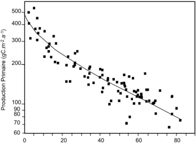
Cette relation a été vérifiée et quantifiée sur des sédiments de surface de l’océan Indien (figure 2.3)(Beaufort et al., 1997). Les données de production primaire sont extraites de l’atlas (Antoine et al., 1995). Ces auteurs ont couplé les images couleurs satellitales, avec des algorithmes permettant d’intégrer la production primaire dans la colonne d’eau.

80 60 40 20 0 60 70 80 90 100 200 300 400 500 Florisphaera profunda (%) Figure 2.3 : Calibration de la relation entre

Florisphaera profunda et la production primaire (d’après (Beaufort et al., 1997)).

Résumé de l’article :

Cette calibration a été appliquée aux comptages de Florisphaera profunda effectués à haute résolution dans la carotte MD97-2141 située dans la mer de Sulu qui enregistre les 200 000 dernières années. Actuellement, la production primaire est linéairement reliée à la vitesse des vents de la mousson d’hiver Est-asiatique. Les variations de production primaire dans cette carotte nous indiquent donc les variations dans l’intensité de la mousson d’hiver Est-Asiatique.

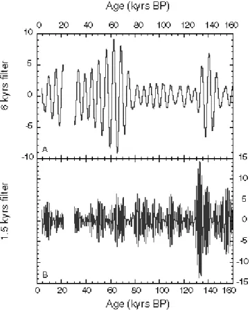
A l’échelle glaciaire-interglaciaire, la production primaire est renforcée pendant les stades glaciaires indiquant un renforcement de la mousson d’hiver en période glaciaire. Pendant le dernier stade glaciaire, huit pics de mousson sont recensés, l’occurrence de ces pics étant également enregistrés dans les séquences loessiques de Chine. Ces pics ne sont pas tous liés aux débâcles massives d’icebergs dans l’Atlantique Nord (événements de Heinrich), la moitié seulement des pics décrits en mer de Sulu étant synchrones avec les événements de Heinrich. Néanmoins, une analyse SSA (‘Singular Spectrum Analysis’), analyse en composantes principales d’un signal temporel, ainsi que des analyses spectrales révèlent qu’à l’échelle des Dansgaard-Oeschger une dynamique commune existe entre la mousson d’hiver Est-asiatique et les températures au Groenland. Dans cet enregistrement, la mousson d’hiver Est-asiatique oscille à des périodes d’environ 6 ka, 4.2-3.4, 2.3 et 1.5 ka. Ce cycle de 1500 ans est présent du stade isotopique marin 6 jusqu’à l’Holocène, sans que le volume des glaces ne module ce cycle. Ceci suggère que les cycles de 1500 ans ne sont pas forcés par les hautes latitudes comme précédemment supposés.

Chapitre 1 : Variabilité millénnale de la mousson d’hiver

Références :

Antoine, D., André, J.-M., and Morel, A., 1995, Oceanic primary production 2. Estimation at global scale from satellite (coastal zone color scanner) chlorophyll: Global Biogeochemical Cycles, v. 10, p. 57.

Beaufort, L., Lancelot, Y., Camberlin, P., Cayre, O., Vincent, E., Bassinot, F., and Labeyrie, L., 1997, Insolation cycles as a major control of equatorial Indian ocean primary production: Science, v. 278, p. 1451-1454.

Behl, R., and Kennet, J.P., 1996, Brief interstadial events in the Santa Barbara basin, NE Pacific, during the past 60 kyr: Nature, v. 379, p. 243-246.

Bianchi, G.G., and McCave, I.N., 1999, Holocene periodicity in North Atlantic climate and deep-ocean flow south of Iceland: Nature, v. 397, p. 515-517.

Bond, G., Showers, W., Chezebiet, M., Lotti, R., Almasi, P., deMenocal, P., Priore, P., Cullen, H., Hajdas, I., and Bonani, G., 1997, A pervasive millenial scale cycle in North-Atlantic holocene and glacial climates: Nature, v. 278, p. 1257-1266.

Dansgaard, W., Johnsen, S.J., Clausen, H.B., Dahl-Jensen, D., Gundestrup, N.S., Hammer, C.U., Hvidberg, C.S., Steffensen, J.P., Sveinbjörnsdottir, A.E., Jouzel, J., and Bond, G., 1993, Evidence for general instability of past climate from a 250 kyr ice-core record: Nature, v. 364, p. 218-220.

Mayewski, P.A., Meeker, L.D., Twickler, M.S., Whitlow, S., Yang, Q., Lyons, W.B., and Prentice, M., 1997, Major features and forcing of high-latitude northern hemisphere atmospheric circulation using a 110,000-year long glaciogeochemical series: Journal of Geophysical Research, v. 102, p. 26345-26366.

Molfino, B., and McIntyre, A., 1990, Precessional forcing of nutricline dynamics in the Equatorial Atlantic: Science, v. 249, p. 766-769.

Okada, H., and Matsuoka, M., 1994, Lower-photic nannoflora as an indicator of the late Quaternary monsoonal palaeo-record in the tropical Indian Ocean, O.D.P. and the Marine Biosphere: Aberystwyth, p. 233-245.

Pisias, N.G., Sancetta, C., and Dauphin, P., 1973, Spectral analysis of late Pleistocene-Holocene sediments: Quaternary Research, v. 3, p. 3-9.

Porter, S.C., and Zhisheng, A., 1995, Correlation between climate events in the North Atlantic and China during the last glaciation: Nature, v. 375, p. 305-308.

Sachs, J.P., and Lehman, S.J., 1999, Subtropical North Atlantic temperatures 60,000 to 30,000 years ago: Science, v. 186, p. 756-759.

Schulz, H., von Rad, U., and Erlenkeuser, H., 1998, Correlation between Arabian Sea and Greenland climate oscillations of the past 110,000 years: Nature, v. 393, p. 54-57.

Stuiver, M., and Braziunas , T.F., 1993, Sun, ocean, climate and atmospheric 14CO2: an evaluation of causal and spectral relationships: The Holocene, v. 3, p. 289-305.

Xiao, J.L., An, Z.S., Liu, T.S., Inouchi, Y., Kumai, H., Yoshikawa, S., and Kondo, Y., 1999, East Asian monsoon variation during the last 130,000 years: evidence from the Loess Plateau of central China and Lake Biwa of Japan: Quaternary Science Reviews, v. 18, p. 147-157.

Millennial-scale dynamics of the East Asian winter monsoon during the last

200,000 years

Thibault de Garidel-Thoron and Luc Beaufort

Centre Européen de Recherche et d'Enseignement en Géosciences de l'Environnement (CEREGE), Aix-en-Provence, France

Braddock K. Linsley and Stefanie Dannenmann

Department of Earth and Atmospheric Sciences, University at Albany, State University of New York, Albany, New York, USA

Abstract: The primary productivity dynamics of the last 200,000 years in the Sulu Sea was reconstructed using the abundance of the coccolithophore Florisphaera profunda in the IMAGES MD97-2141 core. We find that primary productivity was enhanced during glacial periods, which we suggest is due to a stronger East Asian winter monsoon. During the last 80 kyr, eight significant increases in primary productivity (PP) in the Sulu Sea are similar to East Asian winter monsoon changes recorded in Chinese loess. The PP maxima are not linked with Heinrich events (HE) in the North Atlantic, although four PP peaks are synchronous with HE. The PP oscillations have frequencies near those of the Dansgaard–Oeschger cycles in Northern Hemisphere ice records and indicate a teleconnection of the East Asian winter monsoon with Greenland climate. In this Sulu Sea record the East Asian winter monsoon oscillates with periodicities of ~6, 4.2–3.4, 2.3, and 1.5 kyr. In particular, the 1.5 kyr cycle exhibits a strong and pervasive signal from stage 6 to the Holocene without any ice volume modulation. This stationarity suggests that the 1.5 kyr cycle is not driven by some high-latitude forcing.

1. Introduction

The coupling between the atmosphere and the ocean is fundamental to climate dynamics over seasonal to millennial timescales. Variations in this coupling influence the oceanic biosphere and particularly the phytoplankton of the upper ocean layer. In low-latitude areas the phytoplanktonic activity quantified by primary productivity (PP) is correlated to the wind stress dynamics on the sea surface [Nair et al., 1989]. Previous studies have concentrated on long-term changes in the PP [e.g.,

Beaufort et al., 1997; Mix, 1989], but little is known about the millennial-scale dynamics of PP.

At present, we know that during the last glacial stage our climate system went through rapid changes that are well documented in the North Atlantic area. Two major types of abrupt changes have been described. Heinrich events are documented massive iceberg discharges of ice-rafted debris to the North Atlantic deep-sea sediments occurring with a periodicity of ~6–7 kyr [Bond et al., 1992;

Heinrich, 1988]. These events are followed by consecutive abrupt warmings on the Greenland

Chapitre 1 : Variabilité millénnale de la mousson d’hiver

been described in the Greenland ice cores records [Dansgaard et al., 1993]. These oscillations correspond to ~15°C air temperature shifts between a stadial (cold phase) and an interstadial (warm phase) [Jouzel, 1999].

The Heinrich events are correlative with major changes in the climate dynamics recorded worldwide, from the North Atlantic to the Antarctic. In the Asian region the East Asian winter monsoon strengthened during Heinrich events [Porter and Zhisheng, 1995; Xiao et al., 1999]. Planktonic foraminifera assemblage in South China Sea recorded these abrupt changes [Chen and

Huang, 1998; Wang et al., 1999]. In the Sulu Sea the oxygen isotopes ( 18O) of planktonic

foraminifera show important rapid oscillations which appear synchronous with some Heinrich events

[Linsley, 1996].

For the Dansgaard–Oeschger oscillations recorded in ice cores, similar changes are documented in sea surface temperature (SST) reconstructions, percentage of carbonate, magnetic susceptibility, planktonic foraminifera oxygen isotopic composition, and foraminiferal assemblages records from the North Atlantic Ocean (for a review, see Cortijo et al. [2000]). The loess-paleosol record in China exhibits comparable shifts [Chen et al., 1997]. In the Santa Barbara basin a bioturbation index records nearly all stadials and interstadials described in the Greenland record [Behl and Kennet, 1996]. At low latitudes, organic carbon changes in the Arabian Sea appear to correlate with D-O cycles [Schulz et al.,

1998].

To constrain the past millennial variations of low-latitude paleoproductivity, we investigate, at high-resolution, variations in the coccolith assemblages in IMAGES giant piston core MD97-2141 located in the Sulu Sea (Figure 1).

Figure 1. Map of Southeast Asia

and of the marginal seas of the western Pacific. Note location of core MD97-2141 in the Sulu Sea.

The Sulu Sea is located between the Asian continent and the “Western Pacific Warm Pool” (WPWP), where annual SST is above 29°C [Yan et al., 1992]. The climate of the Sulu Sea is strongly

influenced by the East Asian monsoon. The East Asian monsoon results from the different potential heating between the WPWP and the Asian continent. During the boreal winter the main heating source is located in the ocean. The latent heat release associated with intense convective precipitation fuels the meridional circulation. Tropical convection in the western equatorial Pacific is connected to the descending branch over the Siberian region, forming a strong local Hadley cell in the East Asian region [Zhang et al., 1997]. The East Asian winter monsoon winds in the Sulu Sea result from the merging of the northerly East Asian monsoon with the Pacific trade winds over the South China Sea

[McGregor and Nieuwolt, 1998]. East Asian winter monsoon bursts during January to March (Figure

2) can induce blooms of coccolithophorids [Wiesner et al., 1996]. The PP rises correlatively to the wind stress strengthening because of the stronger mixing of the upper ocean (Figure 2) [Nair et al.,

1989]. Thus coccolith assemblages record information on both paleoproductivity changes and also on East Asian winter monsoon variations in the Sulu Sea.

Figure 2. Wind strength in Sulu Sea at 10°N

(Comprehensive Ocean-Atmosphere Data Set (COADS) Atlas) and estimated monthly primary production at the same location from

Antoine and Morel [1996].

2. Material

The 36 m giant piston core IMAGES MD97-2141 (08°47´N, 121°17´E, 3633 m depth) was retrieved during the IPHIS-IMAGES III cruise of the R/V Marion Dufresne in May 1997. This position is located in the vicinity of the Ocean Drilling Program (ODP) Site 769 [Linsley, 1996]. The core is located on the Cagayan ridge, which protects the site from downslope processes, and above the present lysocline depth (~3800 m), allowing for good preservation of carbonates [Linsley et al., 1985; Miao et

al., 1994]. The sediments are composed predominantly of well-preserved nannofossil-foraminifera

Chapitre 1 : Variabilité millénnale de la mousson d’hiver

3. Methods

For coccolith counting, the core was sampled every 2 cm in the upper 6 m of the core, allowing for a resolution of ~70 years, and every 3–4 cm in the lower 30 m for a resolution of ~200–500 years. A smear slide was prepared for each sample, and at least 300 coccoliths were counted for each slide (mean of 357 coccoliths) on a Zeiss Axioscop at a 1000× resolution. Percentages of Florisphaera

profunda (Fp) were computed using the following equation:

The 95% confidence interval for %Fp varies between ±2 and ±6% depending on the percentage of Fp

[Patterson and Fishbein, 1989].

Age model for MD97-2141 Depth in

core (cm)

AMS 14C Age Error*

Calendar Age,

years Species/ Age model

Accession Number 1 4 560 ± 50 4 798 G. ruber (white) OS-16971 10.5 4 210 ± 40 4 286 G. ruber (white) OS-16926 14 4 740 ± 40 4 962 G. ruber (white) OS-16410 29 4 700 ± 55 4 873 G. ruber (white) OS-16972 59 6 020 ± 40 6 416 G. sacculifer (w/out sac) OS-16411 73 6 810 ± 55 7 274 G. sacculifer (w/out sac) OS-16973 85 6 830 ± 90 7 295 G. sacculifer (w/out sac) OS-18401 94 8 850 ± 55 9 455 G. sacculifer (w/out sac) OS-16974 99 10 700 ± 90 12 152 G. sacculifer (w/out sac) OS-16975 120 9 380 ± 160 10 001 G. sacculifer (w/out sac) OS-16977 150 10 200 ± 80 11 045 G. ruber (white) OS-16978 158 10 250 ± 120 11 153 G. sacculifer (w/out sac) OS-16980 162 10 750 ± 50 12 228 G. sacculifer (w/out sac) OS-16979 205.5 11 750 ± 130 13 258 G. sacculifer (w/out sac) OS-17238 212 12 350 ± 65 13 931 G. ruber (white) OS-16412 226.5 13 000 ± 95 14 796 G. ruber (white) OS-16970 244 14 100 ± 70 16 422 G. ruber (white) OS-16413 269 14 750 ± 70 17 200 G. ruber (white) OS-16361 282 15 100 ± 90 17 591 G. sacculifer (w/out sac) OS-17913 339 17 150 ± 140 19 749 G. ruber (white) OS-17914 368 17 650 ± 85 20,430†

G. ruber (white) OS-22672 400 18 850 ± 140 21847† G. sacculifer (w/out sac) OS-17916 440 28 000 ± 130 32,101† G. sacculifer (w/out sac) OS-17882 487 30 900 ± 260 35,146† G. ruber (white) OS-17912 506.5 33 000 ± 310 37,290† G. sacculifer (w/out sac) OS-17917 543 33 600 ± 590 37,893† G. sacculifer (w/out sac) OS-17911 553 34 300 ± 390 38,790†

G. sacculifer (w/out sac) OS-17915 594 36 900 ± 460 41,134† G. sacculifer (w/out sac) OS-17918

920 59 000 SPECMAP 1150 71 000 SPECMAP 1190 80 000 SPECMAP 1400 99 000 SPECMAP 1450 109 000 SPECMAP 1540 115 000 SPECMAP 1650 131 000 SPECMAP 1790 146 000 SPECMAP 1860 151 000 SPECMAP 2000 171 000 SPECMAP 2200 182 000 SPECMAP 2250 196000 SPECMAP * Error is given in 1σ †

Calendar ages have been calculated using a 400 year reservoir correction and applying the Stuiver and Braziunas [1993] calibration curve for samples younger than 20,000 calendar year in age and a U/Th calibration curve for the samples older than 20,000 calendar years [Bard et al., 1993] .

Table 1.

3.1. Age Model

The age model of the core MD97-2141 was developed by Dannenmann et al. [1998] and Oppo et al.

[1998]. It was obtained using 28 accelerator mass spectrometer (AMS) 14C ages on Globigerinoides

ruber and G. sacculifer and by comparison of the planktonic foraminifera 18O curve (on

Globigerinoides ruber and G. sacculifer tests) with the SPECMAP stack [Imbrie et al., 1984] (Table 1). The radiocarbon dates were converted to calendar ages using (1) a correction of 400 years, according to the age reservoir of carbon in the ocean [Bard, 1988], and then (2) the CALIB3 calibration software [Stuiver and Reimer, 1993] to take into account past atmospheric changes in cosmogenic production. All the ages discussed here are calendar ages B.P. The carbon reservoir age in this work is assumed to be invariant with time. We also assumed that the carbon reservoir age changes in the tropical upper oceanic layer where G. ruber and G. sacculifer live are not varying more than ~200 years [Duplessy et al., 1991]. The last appearance datum of G. ruber pink at 1593 cm fits with the Termination II [Thompson et al., 1979], strengthening the validity of the age model (Figure 3). Two ninth-order polynomial regressions were used from the core top to 400 cm and from 440 to 920 cm on the 14C ages and SPECMAP tie points to smooth the sedimentation rate for the last 60 kyr. This smoothing is indispensable for the spectral analyses to avoid spurious peaks linked with sedimentation rates changes.

The average sedimentation rate is ~10.5 cm kyr-1, with maxima during glacial stage 2 of 34 cm kyr-1. For example, the sedimentation rate during the stage 3 is ~30 cm kyr-1, which allows a 70 year resolution (2 cm sampling). A hiatus occurs between 30 and 22 ka (Figure 3). The sedimentation rates are coherent with other records; that is, they are increased during glacial periods and lower during interglacial stages [e.g., Chen and Huang, 1998]. Reduced benthic mixing due to dysaerobic conditions in the Sulu Sea lessens the bioturbation smoothing effect [Kuehl et al., 1993]. The sharp transition in the coccolith record at 14.55 ka, occurs within 2 cm, another argument for a weak bioturbation effect.

3.2. Signal analysis

3.2.1. Spectral analysis. To extract the significant periodicities contained in the PP signal, we performed spectral analysis using different algorithms (Blackman-Tukey, maximum entropy, and multitaper methods) provided in the package Analyseries [Paillard et al., 1996]. The comparison of these different methods allows the discrimination of spurious results due to biases of a particular method. We present only the multitaper method (MTM) results here. The MTM is able to detect low-amplitude oscillations in relatively short time series with a high degree of statistical significance

Chapitre 1 : Variabilité millénnale de la mousson d’hiver

test). This F test is performed on the amplitude to analyze the harmonic oscillations assuming that the signal contains periodic and separated components [Yiou et al., 1997].

Figure 3. (a) Position of accelerator mass spectrometry (AMS) dates on planktonic foraminifera converted in

calendar ages (small triangles) and the SPECMAP tie points used in the stratigraphy (solid circles). Note the hiatus between 400 and 440 cm (shaded area). (b) MD97-2141 18O planktonic foraminifera results at 10 cm intervals (shaded line) compared with the SPECMAP stacked deep-ocean record (thick solid line). (c) MD97-2141 primary productivity (PP) as reconstructed from the coccolithophorid record.

3.2.2. Singular-spectrum analysis. Singular-spectrum analysis (SSA) is designed to extract the information contained in a short, nonstationary, and noisy signal [Vautard and Ghil, 1989]. This method is based on the computing of empirical orthogonal functions in the time domain. SSA can give insight into the dynamics of the underlying system that generates the signal. Using data-adaptive filters which are not period dependant, SSA allows the separation of the noise from the trend and the deterministic oscillations of the signal.

The coccolithophoridae (Prymnesiophycaea) are phytoplanktonic organisms that live in the oceanic photic zone. They are very sensitive to variations in light and nutrient availability, which are both depth dependent. The lower photic zone is darker and richer in nutrients than the upper photic zone. In the tropical ocean the lower photic zone coccolithophoridae community is dominated by Florisphaera

profunda associated with Gladiolithus flabellatus and Algirosphaera robusta, while most of the other

species live in the upper photic zone [Okada and Honjo, 1973].

When the nutricline is shallow, the upper photic zone species dominate the coccolith community, whereas when the nutricline is deeper, the relative proportion of lower photic community is more important. The depth of the nutricline in the low-latitude open ocean is mainly driven by wind intensity. When winds are strong, the upper layers are well mixed, and the nutrients are upwelled into the upper photic zone. Inversely, when wind stress decreases, the mixing is less effective, and the photic zone is depleted in nutrients. This depth relationship between coccolithophorid communities was successfully used by Molfino and McIntyre [1990] to monitor changes in the nutricline depth and has been calibrated to primary productivity by Beaufort et al. [1997] for paleoproductivity reconstructions.

The relationship between the Florisphaera profunda ratio and primary production has already been quantified by Beaufort et al. [1997] with the following equation:

where y is the yearly PP (g C m-2 yr-1) and x is the percent Fp. This equation is based on Indian Ocean low-latitude core tops. We assume that the coccolithophorids' assemblage distributions are homogenous in the intertropical zone. The variations of Fp are in agreement with other paleoproductivity proxies [Beaufort et al., 1997].

4. Results

The present annual PP in the Sulu Sea is 148 g C m-2 yr -1 [Antoine and Morel, 1996], which is close to the average reconstructed PP over the last 200 kyr of 135 g C m-2 yr-1. The PP (data are accessible at http://www.cerege.fr and at ftp://ftp.noaa.ngdc.gov/paleo) oscillates during the last 200 kyr between 81 and 223 g C m-2 yr-1 (Figure 3).

4.1. Glacial-Interglacial Variations

On a glacial-interglacial timescale, PP increases during glacial periods and decreases during interglacials (Figure 3). PP is moderately correlated (r2 = 0.49) with the ice volume curve (SPECMAP stack of Imbrie et al. [1984]). This is shown by the spectral analysis of the paleoproductivity record, which contains orbital frequency peaks of Milankovitch theory (i.e., 1/100 kyr, 1/41 kyr, and ~1/20

Chapitre 1 : Variabilité millénnale de la mousson d’hiver

kyr) (Figure 4) and confirmed by cross-spectral analysis between the PP time series and the SPECMAP stack (not shown). This orbital forcing explains about half of the variance of the PP record. Half of the variance of the PP remains to be explored in the sub-Milankovitch timescale.

Figure 4. Spectral analysis of the

MD97-2141 PP record between 4.1 and 200 ka. Three peaks appear in the spectral analysis computed using the Blackman-Tukey algorithm (solid line) and the maximum entropy algorithm (dotted line), which correspond to orbital frequencies of the Milankovitch theory.

4.2. Sub-Milankovitch Dynamics

4.2.1. Bolling/Allerod and the Younger Dryas event. The last deglaciation is marked by the Younger Dryas event, which interrupts the global warming trend in the Northern Hemisphere. The Younger Dryas seems to be at least hemispheric in extent and has been already described in the Sulu Sea [Kudrass et al., 1991; Linsley and Thunell, 1990]. The Younger Dryas event is also present in the MD97-2141 18O record between 13.5 and 11.5 ka (Figure 3). The paleoproductivity record inferred from Fp is characterized by an abrupt decrease at 14.55 ka (from 170 to ~125 g C m-2 yr-1) to a plateau until 11.5 ka, followed by another decrease to 100 g C m-2 yr-1.

We interpret this PP record to indicate a sharp decrease of the East Asian winter monsoon strength after 14.55 kyr. A similar abrupt transition at 14.5 ka is recorded in the alkenone-sea surface temperature (SST) record of the meridional South China Sea as 1.5°C step [Pelejero et al., 1999a]. Greenland Ice Core Project (GRIP) and Greenland Ice Sheet Project 2 (GISP2) isotopic records also display an abrupt warming at ~14.5 ka. This abrupt warming seems to be at least hemispheric [Bard et

al., 1997]. The sea level rise (meltwater pulse (MWP) Ia of Fairbanks [1989]) was invoked by

Pelejero et al. [1999c] to account for the thermal and terrigenous input changes in the South China

Sea. However, the abruptness of the PP change (<200 years) is not easily attributable to the flooding of the Sundaland. An abrupt drop in the East Asian winter monsoon intensity can explain this PP change in a more plausible manner.

The interpretation of the Younger Dryas event in the Sulu Sea is still controversial. Two main hypotheses were summarized by Anderson and Thunell [1993]: either it reflects a cooling event or it is due to a change in the 18O of seawater. Modern analog technique reconstruction of SST with

planktonic foraminifera does not record enough SST difference during the Younger Dryas to account for the observed isotopic shift [Thunell and Miao, 1996]. So the enrichment is probably due to changes in seawater isotopic composition during the Younger Dryas. The origin of this change is still being debated as an oceanic source [Duplessy et al., 1991] or an atmospheric variation [Anderson and

Thunell, 1993].

The PP plateau during the Allerod and the Younger Dryas is similar to the warming recorded by alkenones records from the cores 17961 and 17964 in the South China Sea (SCS) [Pelejero et al.,

1999a, 1999b]. The Younger Dryas–Allerod SST difference in the SCS is 0.4°C. This corresponds to an increase of ~0.1‰ of the foraminiferal 18O, 20% of the 0.5‰ change observed in Sulu Sea sediments [Linsley, 1996]. Our PP record strengthens the argument that East Asian winter monsoon dynamics during Younger Dryas were not significantly different from the Allerod because of the small measured change in the PP record between the Allerod and the Younger Dryas. Thus the change in planktonic foraminifera 18O composition in the Sulu Sea between the Allerod and the Younger Dryas seems to be mainly due to an isotopic variation in ocean water linked to salinity, after a major change in atmospheric processes 14.5 kyr ago, during the Bolling.

Figure 5. MD97-2141 primary

productivity versus calendar age (solid line) smoothed with a 2 kyr moving average window.

Between 22 and 30 calendar kyr B.P., a hiatus exists in the sediment record identified with

14

C dates (shaded area). The major peaks in PP are numbered from 1 to 8. The Younger Dryas and timing of Heinrich Events in the North Atlantic (shaded area) are shown in toward bottom. The ages for these events are from

Bard [1998] for the Younger Dryas, Thouveny et al. [2000] for North Atlantic Heinrich Events 1–4, and Chapman and Shackleton [1998] for the chronology of H5 and H6.

4.2.2. Millennial-scale PP events during MIS 3. The Heinrich events in the North Atlantic have been correlated to short increases of the East Asian winter monsoon dynamics [Chen et al., 1997;

Porter and Zhisheng, 1995]. In order to compare the millennial variations in the North Atlantic and the

PP variations in the Sulu Sea we smoothed the PP record with a 2 kyr average moving window and resampled at a 100 year time step (Figure 5). This 2 kyr window keeps only the variance at the millennial and longer timescales and attenuates the century-scale variations. During the last 80 kyr the

Chapitre 1 : Variabilité millénnale de la mousson d’hiver

PP record reveals eight events numbered PP1-PP8, some of which may be synchronous with North Atlantic environmental changes (Figure 5). The first one (PP1) at ~8.3 kyr ago is in phase with the early to middle Holocene transition period [Alley et al., 1997]. PP2 matches with Heinrich Event 1 (HE1). PP3 occurs during the Last Glacial Maximum. PP4 seems to correlate with HE4. PP5 and PP6 do not match with any major Heinrich Events, and HE5 is being intercalated between these two PP increases. However, PP5, at ~44 ka is correlated to an increase of the winter monsoon strength recorded in paleoloess from China, dated between 43.3 and 45.2 kyr BP (PL7 of Chen et al. [1997]). PP7 could be related to HE6. PP8 does not match any Heinrich Event. Chen et al. [1997] also describe two events at 59.2–66.2 ka (PL9) and 68.6–71.2 ka (PL10), which may correlate with PP7 and PP8 given age model uncertainties. In conclusion, all PP maxima in the Sulu Sea can be correlated with Chinese loess events and notably events PP5 and PP8 may correspond only with the Chinese loess record. Therefore we conclude that these regional events are indicative of significant changes in the East Asian winter monsoon dynamics. PP1, PP2, PP4, and PP7 match clearly with North Atlantic Heinrich Events. In stage 3, uncertainties in the age model that cannot be smaller than ±2 kyr may explain the relative discrepancy between PP5 or PP6 and HE5 but cannot account for the occurrence of supplementary peaks (PP5 or PP6 and PP8). Our data indicate that the dynamics of the East Asian winter monsoon is not directly linked with the major iceberg discharges in the North Atlantic as stated

by Porter and Zhisheng [1995]. The East Asian winter monsoon exhibits higher-frequency dynamics

than that of the main HE. However, it remains to be determined if a common dynamic is present between the high- and the low-latitude records that is not linked with major icebergs discharges. We next compare the Dansgaard–Oeschger cycles recorded in the Greenland ice core records with our PP record from the Sulu Sea.

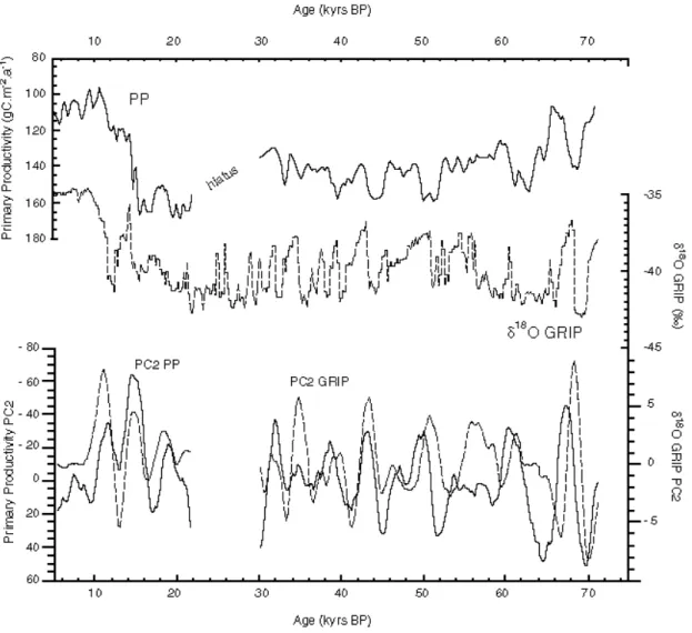
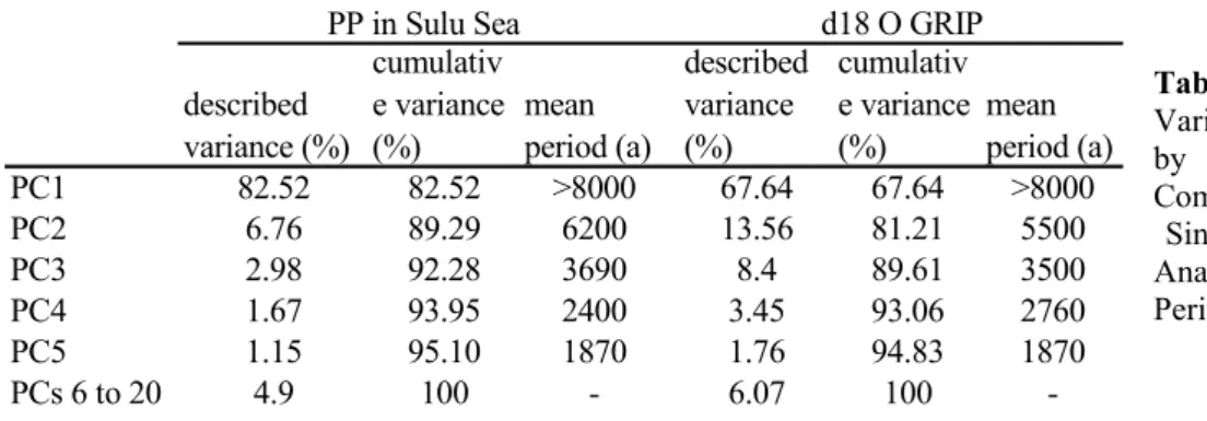
To evaluate Dansgaard–Oeschger scale variability, we performed SSA on the Sulu Sea PP and on the GRIP 18O records to examine the relationships between Greenland climate and East Asian winter monsoon dynamics. For this analysis, we resampled the two records at 200 year time intervals after interpolation. We computed SSA with the Vautard-Ghil autocovariance estimator embedded in 20 dimensions corresponding to 2000 years. The first principal component (PC) in the two records describes the long-term trend, and the second PC shows millennial dynamics (Figure 6 and Table 2). There is a good agreement between the two PC2 records of millennial dynamics in PP and temperature in Greenland during the last 70 kyr. PP increases in the Sulu Sea when temperatures in Greenland decrease. Cross-spectral analysis indicates high coherency between the PC2 of PP and the PC2 of GRIP for the ~6 and 3.5 kyr frequency bands with phases of ~160° and of 140°, which is indicative of the opposite phase described above. This phase relationship is well constrained for the deglaciation by 14_{C ages. The phase cannot be further investigated because of limited synchronization between the ice} core records and the marine records inherent to differences in established chronologies.

A strengthening of the East Asian winter monsoon during the glacial stages is compatible with the conclusions of several studies already carried out in this area [Chen and Huang, 1998; Wang et al.,

1999]. It corresponds to a strengthening of the Hadley cell between the Western Pacific Warm Pool Low and the Siberian High. This mode of atmospheric circulation is compatible with last glacial stage simulations [Kutzbach et al., 1993]. The Siberian Highs are directly connected to the Ferrel cells, which influence the Greenland and Asian climates. This teleconnection should operate via the coupling of these two cells (Ferrel and Hadley) during the winter.

Figure 6. (top) MD97-2141 PP (smoothed; solid line) record versus the 18O record of the GRIP ice core (dotted line). (bottom) PC2 of the PP record (solid line) and PC2 of the 18O record of GRIP (dotted line) as reconstructed by singular spectrum analysis (SSA), which show similar oscillations. Note that both scales in the bottom panel are inverted compared to the top panel.

In conclusion, the lack of a systematic correlation between the Sulu Sea PP and HE indicates that iceberg discharges in the North Atlantic and the East Asian winter monsoon follow different dynamics. However, the correlation between the Greenland climate PC2 and the East Asian winter monsoon PC2 indicates that similar millennial-scale climate variability affects both the Greenland and the Western Pacific climates.