Driver behavior profiling: An investigation
with different smartphone sensors and
machine learning
Jair Ferreira Ju´nior1,2, Eduardo Carvalho1,3, Bruno V. Ferreira1,3, Cleidson de Souza1,2, Yoshihiko Suhara4, Alex Pentland5, Gustavo Pessin1,2*
1 Applied Computing Lab, Instituto Tecnolo´gico Vale, Bele´m – PA, Brazil, 2 Institute of Exact and Natural Sciences, Federal University of Para´, Bele´m – PA, Brazil, 3 SENAI Institute of Innovation – Mineral Technologies, Bele´m – PA, Brazil, 4 Recruit Institute of Technology, Mountain View – CA, United States of America, 5 Media Lab, Massachusetts Institute of Technology, Cambridge – MA, United States of America *[email protected]
Abstract
Driver behavior impacts traffic safety, fuel/energy consumption and gas emissions. Driver behavior profiling tries to understand and positively impact driver behavior. Usually driver behavior profiling tasks involve automated collection of driving data and application of com-puter models to generate a classification that characterizes the driver aggressiveness pro-file. Different sensors and classification methods have been employed in this task, however, low-cost solutions and high performance are still research targets. This paper presents an investigation with different Android smartphone sensors, and classification algorithms in order to assess which sensor/method assembly enables classification with higher perfor-mance. The results show that specific combinations of sensors and intelligent methods allow classification performance improvement.
1 Introduction
Driver behavior strongly impacts traffic security [1] and causes the vast majority of motor vehicle accidents [2]. In 2010, the total economic cost of motor vehicle crashes in the United States was 242 billion [3]. This figure represents the costs for approximately 33 thousand fatali-ties, 4 million nonfatal injuries, and 24 million damaged vehicles. Driver behavior adaptations might increase overall security and lessen vehicle fuel/energy consumption and gas emissions [4,5]. In this context, driver behavior profiling tries to better understand and potentially improve driver behavior, leveraging a safer and more energy aware driving.
Driver monitoring and analysis or driver behavior profiling is the process of automatically collecting driving data (e.g., speed, acceleration, breaking, steering, location) and applying a computational model to them in order to generate a safety score for the driver. Driving data collection may be achieved by several kinds of sensors, from the general ones in smartphones, to dedicated equipment such as monitoring cameras, telematics boxes, and On-Board Diag-nostic (OBD) adapters.
a1111111111 a1111111111 a1111111111 a1111111111 a1111111111 OPEN ACCESS
Citation: Ferreira J, Ju´nior, Carvalho E, Ferreira BV, de Souza C, Suhara Y, Pentland A, et al. (2017) Driver behavior profiling: An investigation with different smartphone sensors and machine learning. PLoS ONE 12(4): e0174959.https://doi. org/10.1371/journal.pone.0174959
Editor: Houbing Song, West Virginia University, UNITED STATES
Received: August 12, 2016 Accepted: March 17, 2017 Published: April 10, 2017
Copyright: © 2017 Ferreira et al. This is an open access article distributed under the terms of the Creative Commons Attribution License, which permits unrestricted use, distribution, and reproduction in any medium, provided the original author and source are credited.
Data Availability Statement:https://github.com/ jair-jr/driverBehaviorDataset.
Funding: This work was supported by MCTI/CT-Info/CNPq, process 277440880/2013-0. The funders had no role in study design, data collection and analysis, decision to publish, or preparation of the manuscript.
Competing interests: The authors have declared that no competing interests exist.
Modern smartphones provide sensors suitable to collect data for driver profile analysis. Pre-vious work [6–8] shows that properly preprocessed and handled smartphone sensors data are an interesting alternative to conventionalblack boxes for the monitoring of driver behavior.
Driver behavior profiling relevance has grown in the last few years. In the insurance tele-matics domain, plans such as Usage-Based Insurance (UBI) or Pay-How-You-Drive (PHYD) make car insurance cheaper by rewarding drivers with good driving scores, instead of only considering group based statistics (e.g., age, gender, marital status) for that end. In the freight management domain, automated, continuous, and real-time driver behavior profiling enables managers to institutionalize campaigns aiming to improve drivers score, and, as a conse-quence, decrease accidents, and increase resource economy, and vehicle lifetime. Furthermore, notifications of unsafe driving events presented to drivers in real-time can help prevent acci-dents. For example, a smartphone app may notify the driver every time she performs an aggressive turn.
Several driver behavior profiling work [9–14] use a smartphone based sensor-fusion to identify aggressive driving events (e.g., aggressive acceleration, aggressive break) as the basis to calculate driver score. Another work [15] uses vehicle sensor data to provide driving tips and assess fuel consumption as a function of driver profile. The machine learning algorithms (MLAs) employed in these papers come down to fuzzy logic or variations of Dynamic Time Warping (DTW). Dynamic Time Warping is an algorithm to find similar patterns in temporal series. It was originally employed in the speech recognition problem [16]. We believe that other MLAs and sensor combination can be applied to the task of identifying aggressive driv-ing events with promisdriv-ing results. In this context, to the best of our knowledge, there is no work that quantitatively assesses and compares the performances combinations of smartphone sensor and MLAs in a real-world experiment.
The main contribution of this work is to evaluate the performance of multiple combina-tions of machine learning algorithms and Android smartphone sensors in the task of detecting aggressive driving events in the context of a real-world experiment. We perform a data-collect-ing phase, drivdata-collect-ing a car, and gathered data from several different sensors while performdata-collect-ing dif-ferent maneuverers. We present how the machine learning methods can be employed in the task and evaluate the accuracy of the combination of sensors and technique aiming to find the best match of sensor/technique to each class of behavior.
The remainder of this paper is organized as follows. In Section 2 we present a comprehen-sive set of works that are related to our proposal, followed by Section 3, in which we present concepts of the employed techniques. Section 4 describes the methodology, presenting the data-gathering phase and the details of how we model the proposed machine learning applica-tion. It is followed by results and discussion (Section 5). Finally, we conclude the paper pre-senting the conclusions and pointing out potential future work.
2 Related work
In this section we describe recent driver behavior profiling work. It is worth noting that several driver behavior profiling solutions are commercially available mowadays, mostly in the insur-ance telematics and freight management domains. Examples include Aviva Drive (www.aviva. co.uk/drive), Greenroad (greenroad.com), Ingenie (www.ingenie.com), Snapshot (www. progressive.com/auto/snapshot), and SeeingMachines (www.seeingmachines.com). However, technical details of these solutions are not publicly available.
Nericell, proposed by Mohan et al. [17], is a Windows Mobile smartphone application to monitor road and traffic conditions. It uses the smartphone accelerometer to detect pot-holes/bumps, and braking events. It also employs the microphone to detect honking, and the
GPS/global system of mobile (GSM) communications to obtain vehicle localization and speed. Braking, bumps and potholes are detected by comparing a set of empirically prede-fined thresholds to abrupt variations of accelerometer data or to their mean over a sliding window of N seconds. No MLA is employed in the detection of such events. Some event detection results in terms of False Positives (FPs) and Fale Negatives (FNs) include: 4.4% FN, and 22.2% FP for breaking events; 23% FN, and 5% FP for bumps/potholes detection at low speed (<25 kmph); and 0% FN and FP for honk detection on an exposed vehicle (e.g., a motorbike).
Dai and colleagues [9] propose an Android application aimed at real time detection and alert of dangerous driving events typically related to Driving Under the Influence (DUI) of alcohol. The application uses the smartphone accelerometer and orientation (yaw, pitch, and roll angles) sensors to detect Abnormal Curvilinear Movements (ACM) and Problems in Maintaining Speed (PMS), which are the two main categories of drunk driving related behav-iors. A series of equations are used to determine lateral and longitudinal acceleration vectors. An ACM event is detected if the difference between maximum and minimum values of lateral acceleration within a 5 seconds time window exceeds an empirical threshold. A PMS is detected if longitudinal acceleration exceeds positive or negative fixed empirical thresholds at any given time. Similarly to [17], no MLA is employed for event detection. Experimental results include: 0% FN, and 0.49% FP for abnormal curvilinear movements; and 0% FN, and 2.90% FP for problems of speed control.
An iPhone application called MIROAD was created by Johnson and Trivedi [10]. MIROAD uses a smartphone based sensor-fusion of magnetometer, accelerometer, gyroscope, and GPS to detect aggressive driving events and accordingly classify driver’s style into aggressive or nonaggressive. Aggressive events are detected by a single classifier based on the DTW algo-rithm. All processing is executed in real-time on the smartphone. Experimental analysis shows that 97% of the aggressive events were correctly detected.
WreckWatch, proposed by White et al. [18], is an Android smartphone-based client/server application to detect car accidents. The client application detects accidents, records related data, and sends them to the server application which can notify relevant authorities. Wreck-Watch client uses data from the accelerometer, GPS, and microphone, with threshold-based filtering to detect an accident. The accident prediction framework is composed of a 11-tuple model of the phone state, and a function that evaluates the model to signal if it represents an accident. Model variables include the maximum acceleration experienced in any direction, and an indication if a loud sound has occurred. One scenario that triggers accident detection is when acceleration, sound, and vehicle speed are all higher than empirical thresholds. Simi-larly to [9,17], no MLA is employed for accident detection. Experiment results show that dropping a phone is unlikely to cause FPs, some accidents may not be detected with smart-phones, and acoustic data is not enough to detect accidents.
Araujo and colleagues [15] present a smartphone application to evaluate fuel consumption efficiency as a function of driver behavior. The application also provides real-time driving hints such asshift gear earlier and accelerating too high. Instead of collecting data from phone sensors, this application uses an OBD Bluetooth adapter and the Torque Pro smart-phone app to collect data (e.g., speed, acceleration, RPM) from vehicle sensors. After data collection, the app extracts a series of features and applies three classifiers (one linear discrimi-nant and two fuzzy systems) to them. All processing is executed in real-time on the
smartphone.
Eren et al. [11] propose an iPhone application to classify driver behavior as either safe or risky based on risky driving events. The application detects sudden turns, lane departures, braking and acceleration events. The sensors used for event detection are the smartphone
accelerometer, gyroscope, and magnetometer. The application uses the endpoint detection algorithm to demarcate start and end times of an event. The demarcated event is then com-pared with template event data by means of the DTW algorithm. Finally, a Bayesian classifier labels a driver’s behavior as safe or risky based on the number of events over time. Experimen-tal results show that 14 out of 15 drivers (93.3%) were correctly classified. It is worth noting that the paper only provides driver classification results. Hence, event classification perfor-mance results are not provided.
The work by Fazeen and colleagues [19] uses an Android smartphone accelerometer and GPS to identify vehicle conditions (speed and shifting), driving patterns (acceleration/deceler-ation and changing lanes), and road condition (smooth, uneven, rough, or containing a bump or pothole). Events are mainly detected by calculating the time duration, difference, and slope between successive accelerometer readings on certain axes and comparing them to empirical fixed/dynamic thresholds. For example, the work states that safe acceleration and deceleration never reach a g-force of more than±0.3g on y-axis. Similarly to [9,17,18], no MLA is
employed for event detection. Experimental results include the following road anomaly classi-fication accuracy: 81.5% for bumps, 72.2% for potholes, 75% for rough roads, 91.5% for smooth roads, and 89.4% for uneven roads.
Castignani et al. [12] propose a driver behavior profiling mobile tool based on fuzzy logic that makes use of accelerometer, magnetometer, and gravity sensors in Android smartphones. This tool classifies driver behavior asNormal, Moderate, and Aggressive, which correspond to a driving score between 0 (best) and 100 (worst). The classification and score are not processed in real-time as sensor data are collected byUBI-Meter mobile application and stored locally on the smartphone. Later on, these data are sent to a remote server on the Internet for processing. The work by Saiprasert and collaborators [13] employs GPS, accelerometer, and magnetome-ter smartphone sensors to profile driver behavior asVery Safe, Safe, Aggressive, and Very Aggressive. This profile is calculated in real-time by detecting relevant driving events. Event detection is performed by a variation of the DTW algorithm [20].
SenseFleet, proposed by Castignani et al. [14], is a driver behavior profiling platform for Android smartphones that is able to detect risky driving events independently from the mobile device and vehicle. The mobile application collects data from accelerometer, magnetometer, gravity sensor, and GPS smartphone sensors and makes use of a fuzzy system to detect risky events such as excessive speed, turning, acceleration, and breaking that might occur in a trip. The application calculates a driving score between 0 (worst) and 100 (best) for each trip as a function of detected risky events. All processing is done in real-time on the smartphone. Authors performed several experiments. In one of these experiments, more than 90% of risky events were correctly identified by the application.
Wahlstrom, Skog and Handel [21] propose a framework for the detection of dangerous vehicle cornering events based on the theoretical likelihood of tire slippage (slipping) and vehi-cle rollover. The Global Navigation Satellite System (GNSS)—a general term for GPS—of Android smartphones is the sole sensor used for event detection. By employing classical mechanics equations, theoretical thresholds for slipping and vehicle rollover are defined. The slipping threshold is defined with respect to tangential and rotational velocities, tangential acceleration, and the coefficient of friction between the vehicle’s tires and the road. The vehicle rollover threshold is defined with respect to the vehicle’s center of gravity, track width, and height. Similarly to [9,17–19], no MLA is employed in event detection. Experimental analysis with GNSS data collected from three different Android smartphone showed an average rate of 13% for both FP and FN as best results.
We have identified some noteworthy points in related work presented here: (i) all papers —except [21]—use sensor-fusion data as input for the event detection algorithms; (ii) the
employed MLAs come down to fuzzy logic [12,14,15] or variations of DTW [10,11,13]; (iii) most recent papers make use of smartphones sensors instead of vehicle or telematics boxes sensors; and (iv) some papers [9,17–19,21] do not use MLAs to detect driving events, instead they employ physical equations or fixed/dynamic thresholds or a combination of both to this end. In our work, we run the machine learning algorithms locally, although, future versions might run on a cloud-based fashion, as presented in [22,23]. Other approaches related to driver behavior are related to social mechanisms, like the evaluation performed by Song and Smith [24], in which driver behavior is investigated in a high-occu-pancy toll lane. A more comprehensive approach about smart and connected communities can be seen in the work by Sun and colleagues [25]. For a more thorough comparison of smartphone-based sensing in vehicles please refer to the work by Engelbrecht and col-leagues [26].
3 Machine learning algorithms
In our evaluation, we compare the performance of four MLAs: Artificial Neural Networks (ANN), Support Vector Machines (SVM), Random Forest (RF), and Bayesian Network (BN). Those MLAs were chosen given their great presence in the literature of classification problems, and the fact that they represent different machine learning “tribes” [27], which ensures a machine learning algorithmic diversity. In this section, basic concepts of the aforementioned MLAs are explained.
3.1 Artificial neural networks
Artificial Neural Networks (ANN) are composed by several computational elements that inter-act through connections with different weights. With inspiration in the human brain, neural networks exhibit features such as the ability to learn complex patterns of data and generalize learned information [28]. The simplest form of an ANN is the Multi Layer Perceptron (MLP) consisting of three layers: the input layer, the hidden layer, and the output layer.
Haykin [29] states that the learning processes of an artificial neural network are determined by how parameter changes occur. Thus, the process of learning an ANN is divided into three parts: (i) the stimulation by extraction of examples from an environment; (ii) the modification of its weights through iterative processes in order to minimize ANN output error; and (iii) the network responds in a new way as a result of the changes that occurred. Parameter configura-tion directly impacts on the process of learning an ANN. Some examples of parameters are: learning rate, momentum rate, stop criteria and form of network training.
3.2 Support vector machines
Support Vector Machines (SVM) [30] are a supervised learning method used for regression and classification. The algorithm tries to find an optimal hyperplane which separates the d-dimensional training data perfectly into its classes. An optimal hyperplane is the one that max-imizes the distance between examples on the margin (border) which separates different classes. These examples on the margin are the so-called “support vectors”.
Since training data is often not linearly separable, SVM maps data into a high-dimensional feature space though some nonlinear mapping. In this space, an optimal separating hyperplane is constructed. In order to reduce computational cost, the mapping will be performed by ker-nel functions, which depend only on input space variables. The most used kerker-nel functions are: linear, polynomial, radial base function (RBF) and sigmoid.
3.3 Random forrest
Random Forests (RF) are sets of decision trees that vote together in a classification. Each tree is constructed by chance and selects a subset of features randomly from a subset of data points. The tree is then trained on these data points (only on the selected characteristics), and the remaining “out of bag” is used to evaluate the tree. Random Forests are known to be effective in preventing overfitting.
Proposed by Leo Breiman [31] its features are: (i) it is easy to implement; (ii) it has good generalization properties; (iii) its algorithm outputs more information than just class label; (iv) it runs efficiently on large data bases; (v) it can handle thousands of input variables without variable deletion; and (vi) it provides estimates of what variables are important in the classification.
3.4 Bayesian networks
According to Ben-Gal [32], Bayesian Networks (BNs) belong to the family of probabilistic graphical models. These graph structures are used to represent knowledge about an uncertain domain. In particular, each node in the graph represents a random variable, while the edges between the nodes represent probabilistic dependencies among the corresponding random variables. Such conditional dependencies in the graph are often estimated using known statis-tic and computational methods. Thus, Bayesian networks combine principles of graph theory, probability theory, and statistics.
4 Methodology
We modeled this work as a multi-label supervised learning classification problem where the labels are driving events types. The goal of this work is to identify the best combination of motion sensor (and its axes), learning algorithm (and its parameters), and number of frames in the sliding window (nf) to detect individual driving event types. To this end, we define an evaluation assembly in the formEA = {1:sensor, 2:sensor axis(es), 3:MLA, 4:MLA configuration, 5:nf}.
An assembly is evaluated by training, testing, and assessing the performance of the classifier generated by the specified MLA (element #3) with its configuration parameters (element #4) over a data set identified by sensor (element #1), its axis(es) (element #2), and number of frames in sliding window (element #5). By changing the value of an element in this assembly, we achieve a different driving event detection performance. Therefore, this assessment evalu-ates several combinations of element values in order to reveal the best performing ones for each driving event type.
Fig 1shows a high level view of our evaluation pipeline. In the first step of the pipeline, smartphone sensor raw data is sampled and translated from the device coordinate system to Earth’s coordinate system (Fig 2). This translation is necessary in order to achieve device posi-tion independence inside the vehicle. Translated sensor data are then stored in the smartphone file system. In the second step, translated sensor data files are retrieved from the smartphone and used as input to generate attribute vector data sets. In the third step, attribute vector data sets are used to train, test and assess MLAs performances. As depicted inFig 1, the first pipe-line step is executed on the smartphone, whereas the second and final steps are executed on a regular computer.
The metric we use to evaluate assembly performance for each driving event type is the area under the ROC curve (AUC) [33,34]. The AUC of a classifier ranges from 0.0 (worst) to 1.0 (best), but no realistic classifier should have an AUC less than 0.5 which is equivalent to
random guessing. Hence, the closer an evaluation assembly AUC is to 1.0, the better it is at detecting a particular driving event type.
In the remainder of this section, Subsection 4.1 presents the detailed evaluation assembly of machine learning and sensors. Subsection 4.2 describes the proposed attribute vector, used as input for the machine learning algorithms. Finally, Subsection 4.3 presents how we performd the data collection in a real-world experiment.
4.1 Evaluation assembly
Thesensor is the first element of the evaluation assembly. It represents one of the following Android smartphone motion sensors: accelerometer (Acc), linear acceleration (LinAcc),
Fig 1. High level view of our evaluation pipeline showing processing steps from raw sensor data sampling to training, testing, and assessing MLAs.
https://doi.org/10.1371/journal.pone.0174959.g001
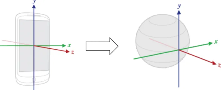
Fig 2. Sensor data are translated from the device coordinate system to Earth’s, in order to achieve device position independence. https://doi.org/10.1371/journal.pone.0174959.g002
magnetometer (Mag), and gyroscope (Gyr). The accelerometer measures the acceleration in meters per second squared (m/s2) applied to the device, including the force of gravity. The
lin-ear acceleration sensor is similar to the accelerometer, but excluding the force of gravity. The magnetometer measures the force of the magnetic field applied to the device in micro-Tesla (μT), and works similar to a magnet. The gyroscope measures the rate of rotation around the device’s axes in radians per second (rad/s). These sensors provide a 3-dimensional (x, y e z) temporal series with nanoseconds precision in the standard sensor coordinate system (relative to the device).
The second element of the evaluation assembly is the sensor axis(es). Available values for this element are (i) all 3 axes; (ii)x axis alone; (iii) y axis alone; and (iv) z axis alone. For exam-ple, the accelerometer originates the following data sets:accelerometer (with data from all three axes),accelerometer_x, accelerometer_y, and accelerometer_z. The only exception to this rule is the magnetometer whosex axis values are always 0 or close after translated to Earth’s coordi-nate system. For that reason, there is nomagnetometer_x data set. As we evaluate data from 3 sensors that originate 4 data sets, and 1 sensor that originates 3 data sets, there is a total of 3⇤4 + 3 = 15 data sets. We separated sensor axes in distinct data sets to observe if any single
axis would emerge as the best to detect a particular driving event type.
The MLA is the third element of the evaluation assembly. As detailed in Section 3, we evalu-ate the classification performance of MLP, SVM, RF, and BN MLAs. We used the WEKA (ver-sion 3.8.0) implementations of these algorithms in conjunction with LIBSVM [35] library (version 3.17). We trained and tested these classifiers using 10-fold cross-validation in order to minimize overfitting.
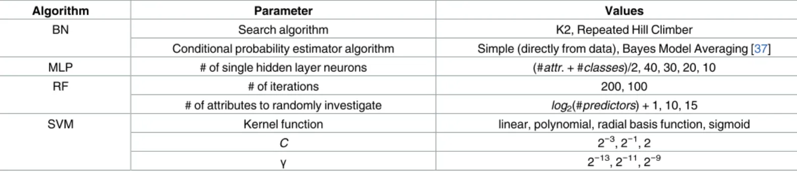
Algorithm configuration is the forth element of the evaluation assembly. We performed a parameter grid search to assess each algorithm with every possible combination of parameter values onTable 1. We set most of the parameter values experimentally, and followed the guide-lines provided in [36] for SVM. We also used WEKA default values for parameters not listed onTable 1.
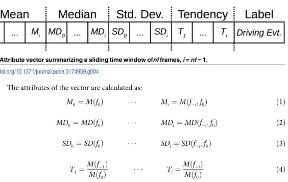
Raw sensor data are basically composed of 3-axes values and a nanosecond timestamp indi-cating the instant the sample was collected. However, we do not send raw sensor data to classi-fiers. Instead, we group sensor time series samples in one-second length frames to compose a sliding time window which is later summarized to originate an attribute vector. As time passes, the window is slided in 1 frame increments over the temporal series as depicted inFig 3. We considerf0as the frame of the current second,f−1as the frame of the previous second, and so
forth down tof−(nf − 1), wherenf (the fifth element of the evaluation assembly) is the number of
frames that compose the sliding time window. We used the followingnf values in this evalua-tion: 4, 5, 6, 7, and 8. These values were defined experimentally so that the sliding window can
Table 1. MLAs configurations.
Algorithm Parameter Values
BN Search algorithm K2, Repeated Hill Climber
Conditional probability estimator algorithm Simple (directly from data), Bayes Model Averaging [37] MLP # of single hidden layer neurons (#attr. + #classes)/2, 40, 30, 20, 10
RF # of iterations 200, 100
# of attributes to randomly investigate log2(#predictors) + 1, 10, 15
SVM Kernel function linear, polynomial, radial basis function, sigmoid
C 2−3, 2−1, 2
γ 2−13, 2−11, 2−9
accommodate the length of collected driving events which range from 2 to 7 seconds depend-ing on how aggressive the event is.
In this work, we assessed the performance of several evaluation assemblies to find the ones that best detect each driving event type. The number of assemblies is the result of all combina-tions of 15 data sets, 5 different values fornf, 4 configurations (Table 1) of the BN algorithm, 5 of the MLP, 6 of the RF, and 36 of the SVM. This results in a total of 15⇤5⇤4 + 15⇤5⇤5 +
15⇤5⇤6 + 15⇤5⇤36 = 3825 evaluation assemblies.
4.2 Attribute vector
An attribute vector is the summarization of the sliding window depicted inFig 3. One instance of the attribute vector is generated for every time window that contains a driving event on it. Correspondingly, if there is no driving event for a particular time window, no attribute vector instance is generated.
We create an instance of the attribute vector by calculating the mean (M)Eq (1), median (MD)Eq (2), standard deviation (SD)Eq (3), and the increase/decrease tendency (T)Eq (4)
over sensor data samples in the frames composing the time window. The number of attri-butes in the vector is dependent on the number of frames in the sliding window (nf). There arenf mean, median, and standard deviation attributes, and nf − 1 tendency attributes.
Fig 4depicts the structure of an attribute vector for a single axis of sensor data. When the data set is composed of more than one axis, the attribute vectors for each axis are simply concatenated and only the class label attribute of the last vector is preserved as they all have the same value.
Fig 3. Time window composed of nf one-second frames which group raw sensor data samples. The time window slides in 1 frame increments as time passes. f0is the frame of the current second, f−1is the frame
of the previous second, and so forth down to f−i, where i = nf − 1.
The attributes of the vector are calculated as: M0 à MÖf0Ü Mi à MÖf i;f0Ü Ö1Ü MD0à MDÖf0Ü MDià MDÖf i;f0Ü Ö2Ü SD0à SDÖf0Ü SDià SDÖf i;f0Ü Ö3Ü T1 à MÖf 1Ü MÖf0Ü TiàMÖfMÖfiÜ 0Ü Ö4Ü
Wherei = [0..(nf − 1)], SF(fj) is a summarizing function (mean, median, or standard deviation)
applied over the samples of thejthframe, andSF(f
j,fk) is a summarizing function applied over
the samples from thejthto thekthframe (j < k).
The class label attribute of the vector comes from the driving events ground-truth, as described later in Section 4.3. The class label is the driving event whose start timestamp is between the first timestamp of the samples in framef−(nf − 1)and the last timestamp of the
sam-ples in framef0. We should mention that attribute vectors originating from different driving
trips can be grouped together in the same data set as they are time-independent.
It is important to highlight that a single driving event raw sensor data sample generatesnf attribute vector instances. This occurs because the window frame that contains the start time-stamp of the event changes its position in the window as it slides. Therefore, if there ares sam-ples of a particular driving event type, there will bes⇤nf attribute vector instances for that
same event type. This behavior allows for multiple windows to capture different portions or signatures of the same event.
4.3 Data collection in a real-world experiment
We performed a real-world experiment in order to collect sensor data for driving events. In this experiment, an Android application recorded smartphone sensor data while a driver exe-cuted particular driving events. We also recorded the start and end timestamps of the driving events to generate the ground-truth for the experiment.
We performed the experiment in 4 car trips of approximately 13 minutes each in average. The experiment conditions were the following: (i) the vehicle was a 2011 Honda Civic; (ii) the smartphone was a Motorola XT1058 with Android version 5.1; (iii) the smartphone was fixed on the car’s windshield by means of a car mount, and was neither moved nor operated while collecting sensor data; (iv) the motion sensors sampling rate varied between 50 and 100 Hz, depending on the sensor; (v) two drivers with more than 15 years of driving experience exe-cuted the driving events; and (vi) the weather was sunny and the roads were dry and paved with asphalt.
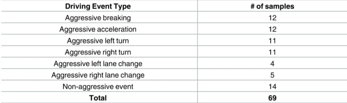
The driving events types we collected in this experiment were based on the events in [13]. Our purpose was to establish a set of driving events that represents usual real-world events
Fig 4. Attribute vector summarizing a sliding time window ofnf frames, i = nf − 1. https://doi.org/10.1371/journal.pone.0174959.g004
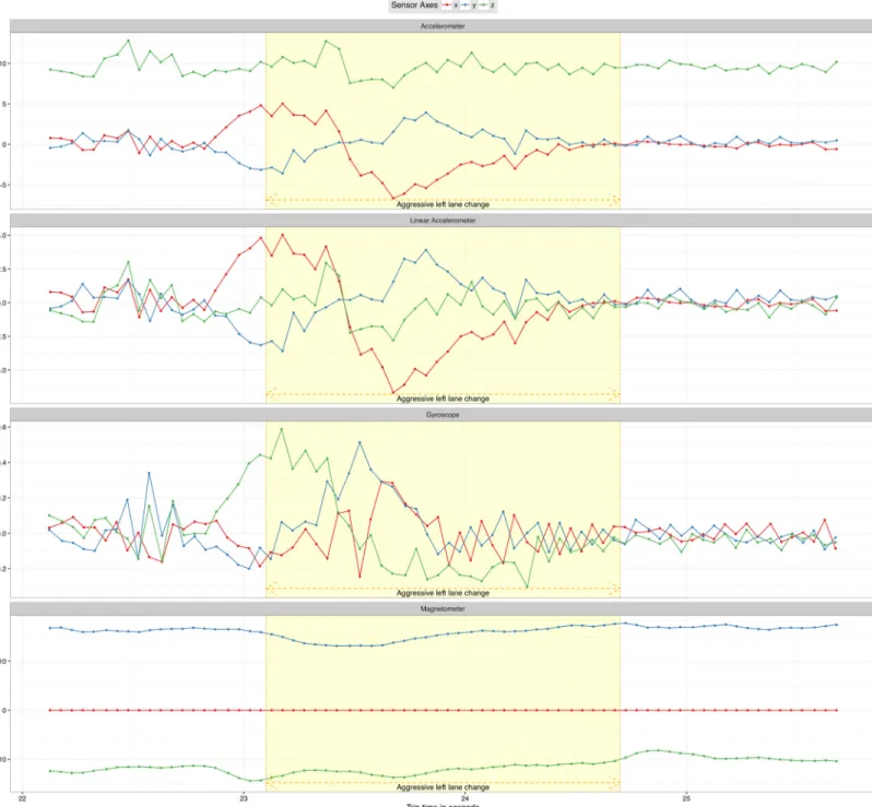
such as breaking, acceleration, turning, and lane changes.Table 2shows the 7 driving events types we used in this work and their number of collected samples.Fig 5shows sensor data for an aggressive left lane change event as it is captured by the four sensors used in this evaluation.
5 Results
We executed all combinations of the 4 MLAs and their configurations described onTable 1
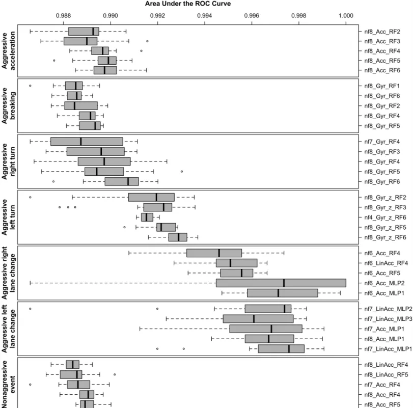
over the 15 data sets described in Section 4.3 using 5 differentnf values. We trained, tested, and assessed every evaluation assembly with 15 different random seeds. Finally, we calculated the mean AUC for these executions, grouped them by driving event type, and ranked the 5 best performing assemblies in the boxplot displayed inFig 6. This figure shows the driving events on the left-hand side and the 5 best evaluation assemblies for each event on the right-hand side, with the best ones at the bottom. The assembly text identification inFig 6encodes, in this order: (i) thenf value; (ii) the sensor and its axis (if there is no axis indication, then all sensor axes are used); and (iii) the MLA and its configuration identifier.
In light of the these results, we can draw a few conclusions in the context of the performed experiment. Firstly, MLAs perform better with highernf values (i.e., bigger sliding window sizes). Of the 35 best performing assemblies, 23 havenf = 8, 6 have nf = 7, 5 have nf = 6, and only 1 hasnf = 4.
Secondly, the gyroscope and the accelerometer are the most suitable sensors to detect the driving events in this experiment. On the other hand, the magnetometer alone is not suitable for event detection as none of the 35 best assemblies use that sensor. Also, using all sensor axes performs better in a general way than using a single axis. The only exception being thez axis of the gyroscope that alone best detects aggressive left turns.
Thirdly, RF is by far the best performing MLA with 28 out of 35 best assemblies. The second best is MLP with 7 best results. RF dominates the top 5 performances for nonaggressive events, and aggressive turns, breaking, and acceleration. However, MLP is better at aggressive lane changes. BN and SVM were not ranked in the best 35 performing assemblies.
Fourthly, MLP configuration #1 was the best performing. In this configuration, the number of neurons in the hidden layer is defined as (#attr. + #classes)/2. This is also the default WEKA configuration. For RF, configurations #6 (# of iterations = 200; # of attributes to randomly investigate = 15), and #5 (# of iterations = 200; # of attributes to randomly investigate = 10) gave the best results.
Finally, we found a satisfactory and equivalent performance in the top 35 ranked evaluation assemblies. This is true because the difference between the worst AUC mean (0.980 for the aggressive breaking event) and the best one (0.999 for the aggressive right lane change event) is only 0.018. A difference that is not significant in the context of this experiment.
Table 2. Driving event types and number of samples.
Driving Event Type # of samples
Aggressive breaking 12
Aggressive acceleration 12
Aggressive left turn 11
Aggressive right turn 11
Aggressive left lane change 4
Aggressive right lane change 5
Non-aggressive event 14
Total 69
6 Conclusions and future work
In this work we presented a quantitative evaluation of the performances of 4 MLAs (BN, MLP, RF, and SVM) with different configurations applied in the detection of 7 driving event types using data collected from 4 Android smartphone sensors (accelerometer, linear acceleration, magnetometer, and gyroscope). We collected 69 samples of these event types in a real-world experiment with 2 drivers. The start and end times of these events were recorded serve as the
Fig 5. Aggressive lane change event data captured by the four sensors used in this evaluation. https://doi.org/10.1371/journal.pone.0174959.g005
Fig 6. Top 5 best AUC assemblies grouped by driving event type as the result of 15 MLA train/test executions with different random seeds. Values closer to 1.0 are better. Driving events are on the left-hand side and assemblies are on the right-hand side. Assemblies with the best mean AUC are closer to the bottom.
experiment ground-truth. We also compared the performances when applying different slid-ing time window sizes.
We performed 15 executions with different random seeds of 3865 evaluation assemblies of the formEA = {1:sensor, 2:sensor axis(es), 3:MLA, 4:MLA configuration, 5:number of frames in sliding window}. As a result, we found the top 5 performing assemblies for each driving event type. In the context of our experiment, these results show that (i) bigger window sizes perform better; (ii) the gyroscope and the accelerometer are the best sensors to detect our driving events; (iii) as general rule, using all sensor axes perform better than using a single one, except for aggressive left turns events; (iv) RF is by far the best performing MLA, followed by MLP; and (v) the performance of the top 35 combinations is both satisfactory and equivalent, varying from 0.980 to 0.999 mean AUC values.
As future work, we expect to collect a greater number of driving events samples using dif-ferent vehicles, Android smartphone models, road conditions, weather, and temperature. We also expect to add more MLAs to our evaluation, including those based on fuzzy logic and DTW. Finally, we intend use the best evaluation assemblies observed in this work to develop an Android smartphone application which can detect driving events in real-time and calculate the driver behavior profile.
Author Contributions
Conceptualization: JFJ CdS YS AP GP. Data curation: JFJ EC BVF. Investigation: JFJ EC BVF. Methodology: JFJ CdS YS AP GP. Software: JFJ GP.Writing – original draft: JFJ EC BVF CdS YS AP GP.
References
1. Xiaoqiu F, Jinzhang J, Guoqiang Z. Impact of Driving Behavior on the Traffic Safety of Highway Inter-section. In: Measuring Technology and Mechatronics Automation (ICMTMA), 2011 Third International Conference on. vol. 2; 2011. p. 370–373.
2. Evans L. Traffic safety. Science Serving Society; 2004.
3. Blincoe L, Miller TR, Zaloshnja E, Lawrence BA. The Economic and Societal Impact of Motor Vehicle Crashes, 2010 (Revised). National Highway Traffic Safety Administration; 2015.
4. Haworth N, Symmons M. Haworth, MS. Driving to Reduce Fuel Consumption and Improve Road Safety. Road Safety Research, Policing and Education Conference, 2001, Melbourne, Victoria, Austra-lia. 2001;(5):7.
5. Van Mierlo J, Maggetto G, Van de Burgwal E, Gense R. Driving style and traffic measures-influence on vehicle emissions and fuel consumption. Proceedings of the Institution of Mechanical Engineers, Part D: Journal of Automobile Engineering. 2005; 218:43–50.
6. Paefgen J, Kehr F, Zhai Y, Michahelles F. Driving Behavior Analysis with Smartphones: Insights from a Controlled Field Study. In: Proceedings of the 11th International Conference on Mobile and Ubiquitous Multimedia. MUM’12. New York, NY, USA: ACM; 2012. p. 36:1–36:8.
7. Skog I, Handel P, Ohlsson M, Ohlsson J. Challenges in smartphone-driven usage based insurance. In: Global Conference on Signal and Information Processing (GlobalSIP), 2013 IEEE; 2013. p. 1135– 1135.
8. Ha¨ndel P, Ohlsson J, Ohlsson M, Skog I, Nygren E. Smartphone-Based Measurement Systems for Road Vehicle Traffic Monitoring and Usage-Based Insurance. Systems Journal, IEEE. 2014; 8 (4):1238–1248.https://doi.org/10.1109/JSYST.2013.2292721
9. Dai J, Teng J, Bai X, Shen Z, Xuan D. Mobile phone based drunk driving detection. In: 2010 4th Interna-tional Conference on Pervasive Computing Technologies for Healthcare; 2010. p. 1–8.
10. Johnson DA, Trivedi MM. Driving style recognition using a smartphone as a sensor platform. In: Intelli-gent Transportation Systems (ITSC), 2011 14th International IEEE Conference on; 2011. p. 1609– 1615.
11. Eren H, Makinist S, Akin E, Yilmaz A. Estimating driving behavior by a smartphone. In: Intelligent Vehi-cles Symposium (IV), 2012 IEEE; 2012. p. 234–239.
12. Castignani G, Frank R, Engel T. Driver behavior profiling using smartphones. In: Intelligent Transporta-tion Systems (ITSC), 2013 16th InternaTransporta-tional IEEE Conference on; 2013. p. 552–557.
13. Saiprasert C, Thajchayapong S, Pholprasit T, Tanprasert C. Driver behaviour profiling using smart-phone sensory data in a V2I environment. In: Connected Vehicles and Expo (ICCVE), 2014 Interna-tional Conference on; 2014. p. 552–557.
14. Castignani G, Derrmann T, Frank R, Engel T. Driver Behavior Profiling Using Smartphones: A Low-Cost Platform for Driver Monitoring. Intelligent Transportation Systems Magazine, IEEE. 2015; 7(1):91– 102.https://doi.org/10.1109/MITS.2014.2328673
15. Araujo R, Igreja A, de Castro R, Araujo RE. Driving coach: A smartphone application to evaluate driving efficient patterns. In: Intelligent Vehicles Symposium (IV), 2012 IEEE; 2012. p. 1005–1010.
16. Sakoe H, Chiba S. Dynamic programming algorithm optimization for spoken word recognition. Acous-tics, Speech and Signal Processing, IEEE Transactions on. 1978; 26(1):43–49.https://doi.org/10.1109/ TASSP.1978.1163055
17. Mohan P, Padmanabhan VN, Ramjee R. Nericell: Rich Monitoring of Road and Traffic Conditions Using Mobile Smartphones. In: Proceedings of the 6th ACM Conference on Embedded Network Sensor Sys-tems. SenSys’08. New York, NY, USA: ACM; 2008. p. 323–336.
18. White J, Thompson C, Turner H, Dougherty B, Schmidt DC. WreckWatch: Automatic Traffic Accident Detection and Notification with Smartphones. Mob Netw Appl. 2011; 16(3):285–303.https://doi.org/10. 1007/s11036-011-0304-8
19. Fazeen M, Gozick B, Dantu R, Bhukhiya M, Gonza´lez MC. Safe Driving Using Mobile Phones. IEEE Transactions on Intelligent Transportation Systems. 2012; 13(3):1462–1468.https://doi.org/10.1109/ TITS.2012.2187640
20. Saiprasert C, Pholprasit T, Pattara-Atikom W. Detecting driving events using smartphone. In: Proceed-ings of the 20th ITS World Congress; 2013.
21. Wahlstro¨m J, Skog I, Ha¨ndel P. Detection of Dangerous Cornering in GNSS-Data-Driven Insurance Telematics. IEEE Transactions on Intelligent Transportation Systems. 2015; 16(6):3073–3083.https:// doi.org/10.1109/TITS.2015.2431293
22. Shojafar M, Cordeschi N, Baccarelli E. Energy-efficient adaptive resource management for real-time vehicular cloud services. IEEE Transactions on Cloud computing. 2016; PP(99):1–1.https://doi.org/10. 1109/TCC.2016.2551747
23. Wei W, Fan X, Song H, Fan X, Yang J. Imperfect information dynamic stackelberg game based resource allocation using hidden Markov for cloud computing. IEEE Transactions on Services Comput-ing. 2016; PP(99):1–1.https://doi.org/10.1109/TSC.2016.2528246
24. Song H, Smith BL. Empirical investigation of the impact of high-occupancy-toll operations on driver behavior. In: Transportation Research Board 88th Annual Meeting. 09-1462; 2009.
25. Sun Y, Song H, Jara AJ, Bie R. nternet of things and big data analytics for smart and connected commu-nities. IEEE Access. 2016; 4:766–773.https://doi.org/10.1109/ACCESS.2016.2529723
26. Engelbrecht J, Booysen MJ, van Rooyen GJ, Bruwer FJ. Survey of smartphone-based sensing in vehi-cles for intelligent transportation system applications. IET Intelligent Transport Systems. 2015; 9 (10):924–935.https://doi.org/10.1049/iet-its.2014.0248
27. Domingos P. The Master Algorithm: How the Quest for the Ultimate Learning Machine Will Remake Our World. Basic Books. Basic Books; 2015.
28. Zhao C, Gao Y, He J, Lian J. Recognition of driving postures by multiwavelet transform and multilayer perceptron classifier. Engineering Applications of Artificial Intelligence. 2012; 25(8):1677–1686.https:// doi.org/10.1016/j.engappai.2012.09.018
29. Haykin S. Neural networks and learning machines. vol. 3. Pearson Upper Saddle River, NJ, USA:; 2009.
30. Vapnik VN. The nature of statistical learning theory. Statistics for engineering and information science. New York: Springer; 2000.
31. Breiman L. Random forests. Machine learning. 2001; 45(1):5–32.https://doi.org/10.1023/ A:1010933404324
32. Ben-Gal I. Bayesian Networks. John Wiley & Sons, Ltd; 2008.https://doi.org/10.1002/9780470061572. eqr089
33. Bradley AP. The Use of the Area Under the ROC Curve in the Evaluation of Machine Learning Algo-rithms. Pattern Recogn. 1997; 30(7):1145–1159.https://doi.org/10.1016/S0031-3203(96)00142-2 34. Fawcett T. An Introduction to ROC Analysis. Pattern Recogn Lett. 2006; 27(8):861–874.https://doi.org/
10.1016/j.patrec.2005.10.010
35. Chang CC, Lin CJ. LIBSVM: A library for support vector machines. ACM Transactions on Intelligent Systems and Technology. 2011; 2:27:1–27:27.https://doi.org/10.1145/1961189.1961199
36. Hsu CW, Chang CC, Lin CJ. A practical guide to support vector classification. Department of Computer Science, National Taiwan University; 2003.
37. Hoeting JA, Madigan D, Raftery AE, Volinsky CT. Bayesian Model Averaging: A Tutorial. Statistical Sci-ence. 1999; 14(4):382–417.