Dorsal Stream: From Algorithm To Neuroscience
by
Hueihan Jhuang
Submitted to the Department of Electrical Engineering and Computer
Science
in partial fulfillment of the requirements for the degree of
Doctor of Philosophy
at the
MASSACHUSETTS INSTITUTE OF TECHNOLOGY
ARC$NES
MASSACHUSETTS INSME' OF TECHNOLOGYJUN 17 2011
LIBRARIES
June 2011
@
Massachusetts Institute of Technology 2011. All rights reserved.
Author ...
Department of Electrical Engineering and Computer Science
March 15, 2011
Certified by
...
Tomaso Poggio
Professor
Thesis Supervisor
Accepted by...
...
iesne A. Kolodziejski
Chairman, Department Committee on Graduate Students
Dorsal Stream: From Algorithm To Neuroscience
by
Hueihan Jhuang
Submitted to the Department of Electrical Engineering and Computer Science on March 15, 2011, in partial fulfillment of the
requirements for the degree of Doctor of Philosophy
Abstract
The dorsal stream in the primate visual cortex is involved in the perception of motion and the recognition of actions. The two topics, motion processing in the brain, and action recognition in videos, have been developed independently in the field of neuroscience and computer vision. We present a dorsal stream model that can be used for the recognition of actions as well as explaining neurophysiology in the dorsal stream.
The model consists of a spatio-temporal feature detectors of increasing complexity: an input image sequence is first analyzed by an array of motion sensitive units which, through a hierarchy of processing stages, lead to position and scale invariant representation of motion in a video sequence. The model outperforms or on par with the state-of-the-art computer vision algorithms on a range of human action datasets.
We then describe the extension of the model into a high-throughput system for the recognition of mouse behaviors in their homecage. We provide software and a very large manually annotated video database used for training and testing the system. Our system outperforms a commercial software and performs on par with human scoring, as measured from the ground-truth manual annotations of more than 10 hours of videos of freely behav-ing mice.
We complete the neurobiological side of the model by showing it could explain the motion processing as well as action selectivity in the dorsal stream, based on comparisons between model outputs and the neuronal responses in the dorsal stream. Specifically, the model could explain pattern and component sensitivity and distribution [161], local motion integration [97], and speed-tuning [144] of MT cells. The model, when combining with the ventral stream model [173], could also explain the action and actor selectivity in the STP area.
There exists only a few models for the motion processing in the dorsal stream, and these models were not be applied to the real-world computer vision tasks. Our model is one that agrees with (or processes) data at different levels: from computer vision algorithm, practical software, to neuroscience.
Thesis Supervisor: Tomaso Poggio Title: Professor
Acknowledgments
Since my advisor Prof. Tomaso Poggio firstly told me "you are ready to graduate" in 2009, I have been imagining about writing acknowledgments, but in reality I have only one hour before the due time of my thesis to actually write it.
Living in a foreign country, speaking a foreign language for almost six years is defi-nitely not something I have been planning since my childhood. It was a bit scary in the beginning, but thanks to all the CBCL members and my friends here, it has tuned out to be a very pleasant experience and has became an important part of my life.
Tomaso Poggio, my supervisor, Lior Wolf and Thomas Serre, postdocs (now profes-sors) whom I've been working with, have been leading me and my research with their patience, intelligence and creativity. Especially Tommy and Thomas, they have opened the door to neuroscience for me, a student with EE background, and their research styles and ways of thinking have influenced me very deeply.
Sharat Chikkerur has been a very supportive friend. We joined CBCL at the same day, took many courses together, and stayed overnight to do final projects. Gadi Geiger is like a grandpa and Jim Mutch is like a brother that I never had, listening to my secrets and troubles in life. I also want to thank all my current and former labmates, Kathleen Sullivan, Tony Ezzat, Stanley Bileschi, Ethan Meyers, Jake Bouvrie, Cheston Tan, Lorenzo Rosasco, Joel Leibo, Charlie Fronger and Nicholas Edelman. Although we never hang out for some big trip to something like Cape Cod like other labs, although I never play foosball/pool with everybody, I always enjoy their company at CBCL. All of them together make the lab an interesting and warm place where I'm willing to spend 24 hours a day and 7 days a week, like how Tommy introduced me at my defense.
Friends outside CBCL also play an important role in my life. Jiankang Wang, who specifically asked to be acknowledged, is my roommate and a very good friend for years. Our brains oscillate at very similar frequency (hers is a bit higher than mine) which makes us laugh at the same implicit jokes, even when I was in the most difficult situation. Tobias Denninger is a very dear and extremely smart friend of mine. He has been giving me a lot of mental support as well as useful feedbacks for my research. He also shows me some
aspects of life which I would never find out by myself. I want to thank Chia-Kai Liang, Ankur Sinha, Andrew Steele (also a collaborator), ROCSA friends, my friends in Taiwan for their care.
My parents have served as my night line as well as day line; they are always ready to listen to all the details of my everyday life. They have been giving me, for the past 27 years, endless love and strong mental support. I simply cannot imagine life without them.
Contents
1 Introduction 27
1.1 The problem . . . 27
1.2 The approach . . . 28
1.3 Outline & summary of thesis chapters . . . 29
1.4 Contribution . . . 31
2 The Model 37 2.1 Motivation from physiology . . . 37
2.2 Background: hierarchical models for object recognition . . . 39
2.3 The model . . . 41
2.3.1 Si . . . 41
2.3.2 C1 . . . 42
2.3.3 S2 . . . 43
2.3.4 C2 . . . .. . -. . . . 44
3 A Biologically Inspired System for Action recognition 45 3.1 The problem . . . 46 3.2 Previous work . . . 47 3.2.1 Global representation . . . 48 3.2.2 Local representation . . . 48 3.3 System Overview . . . 49 3.4 Representation stage . . . . 50
3.4.1 Motion-direction sensitive Si units . . . . 50 7
3.4.2 3.4.3 3.4.4 3.4.5 3.4.6 3.5 Classifi 3.6 Experi 3.6.1 3.6.2 3.6.3 3.6.4 3.7 Conclu C1 stage . . . .
S2 templates of intermediate complexity .
S2 template matching . . . .
C2 feature selection with zero-norm SVM
S3 and C3 stage . . . . cation stage . . . . ments . . . . Preprocessing . . . . Datasets . . . . Benchmark algorithms . . . . Results . . . . sion . . . . 4 HMDB: A Large Video Database for Human
4.1 Introduction . . . .
4.2 Background: existing action datasets . . . 4.3 The Human Motion DataBase (HMDB51)
4.3.1 Database collection . . . .
4.3.2 Annotations . . . .
4.3.3 Training and test set generation
4.3.4 Videos normalization . . . .
4.3.5 Videos stabilization . . . .
4.4 Comparison with other action datasets . .
4.5 Benchmark systems . . . .
4.5.1 HOG/HOF features . . . .
4.5.2 C2 features . . . .
4.6 Evaluation . . . .
4.6.1 Overall recognition performance
4.6.2 Robustness of the benchmarks .
4.6.3 Shape vs. motion information
4.7 Conclusion . . . 81
5 A Vision-based Computer System for Automated Home-Cage Behavioral
Phe-notyping of Mice
Introduction . . . . Background: automated Systems for Mice Behavior Analysis .
5.3 Dataset collection and its challenges . . . .
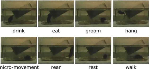
5.3.1 Behavior of interest and definition . . . . .
5.3.2 Datasets . . . . 5.3.3 Annotation . . . . 5.3.4 Challenge . . . . 5.4 System Overview . . . . 5.4.1 Feature Computation . . . . 5.4.2 Classification . . . .
5.5 Experiments and the results . . . .
5.5.1 Training and Testing the system . . . .
5.5.2 Results for the feature computation module
5.5.3 Results for the classification module . . . .
5.6 Application . . . . . . . 8 9 . . . 9 0 . . . 9 1 . . . 9 3 . . . 9 4 . . . 9 6 . . . 9 8 . . . 9 8 . . . 9 9 . . . 103 . . . 1 10
5.6.1 Characterizing the home-cage behavior of diverse inbred mo strains...
5.6.2 Patterns of behaviors of multiple strains . . . .
5.7 Extension of the system to more complex behaviors and environments
5.7.1 Extension to complex behaviors . . . .
5.7.2 Extension to more complex environments . . . .
5.8 Conclusion . . . .
5.9 Future work . . . .
use
6 Towards a Biologically Plausible Dorsal Stream Model
6.1 Introduction . . . .
6.1.1 Organization of the dorsal stream . . . .
5.1 5.2 . .. 110 . . . 113 . . . 114 . . . 114 . . . 115 . . . 117 . . . 118 123 124 124
6.1.2 Motion processing in the dorsal stream . . . .
6.1.3 The problem . . . .
6.1.4 The interpretation of velocity in the frequency domain
6.2 The Model.
6.3 Comparing C2 units with MT cells . . . .
6.3.1 Introduction: directional tuning . . . .
6.3.2 Introduction: speed tuning . . . .
6.3.3 Summary . . . .
6.3.4 Previous computational models . . . .
6.3.5 Two constraints for modeling MT PDS cells
6.3.6 Why our model could explain MT cells . .
6.3.7 Results . . . .
6.3.8 Comparison with other MT models . . . .
6.3.9 Discussion . . . .
6.4 Comparing "ventral + dorsal C2 units" with STP cel
6.4.1 Introduction . . . . 6.4.2 Results . . . . 6.5 Conclusion . . . . [s 124 127 129 131 134 134 140 142 143 145 146 153 164 165 167 167 169 171 . . . .
List of Figures
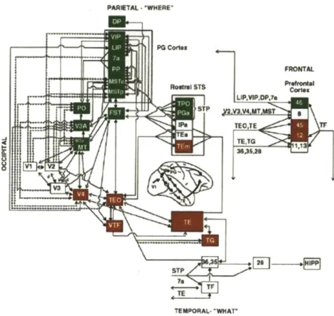
1-1 Visual processing in monkeys. Areas in the dorsal stream are shown in green, and areas in the ventral stream are shown in red. Lines connecting
the areas indicate known anatomical connections, modified from [201]. . . 29
2-1 A possible scheme for explaining the elongated subfields of simple
recep-tive field. Reprinted from [69]. . . . . 38
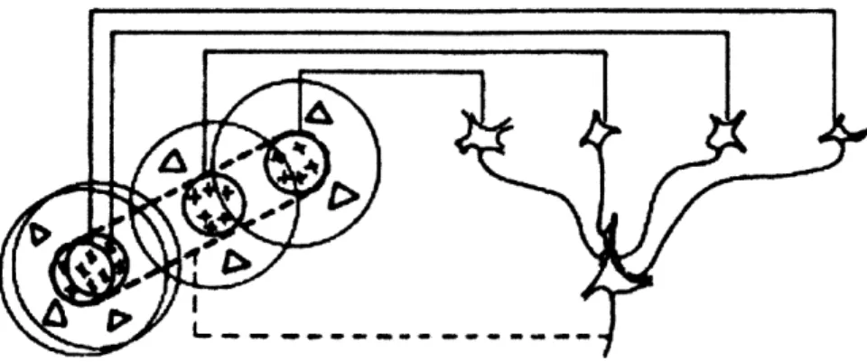
2-2 A possible scheme for explaining the organization of complex receptive
fields. Reprinted from [69]. . . . 38
2-3 HMAX. Figure reprinted from [152] . . . 40
2-4 The structure of the proposed model. The model consists of a hierarchy of layers with template matching operations (S layer) and max pooling oper-ations (C layer). The two types of operoper-ations increase the selectivity and invariance to position and scale change. . . . 42 3-1 Global space-time shapes of "jumping-jack", "walking", and "running".
Figure reprinted from [9] . . . 48 3-2 Local space-time interest points detected from a space-time shape of a
mouse. Figure reprinted from [36] . . . 49
3-3 Sketch of the model for action recognition (see text for details). . . . 50
3-4 An illustration of a dense S2 template [171] (a) vs. a sparse S2 template
[119] (b). . . . 53
3-5 Sample videos from the mice dataset (1 out 10 frames displayed with a
frame rate of 15 Hz) to illustrate the fact that the mice behavior is minute. 56
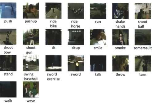
4-1 Illustrations of the 51 actions in the HMDB5 1, part I. . . . 64
4-2 Illustrations of the 51 actions in the HMDB5 1, part II. . . . 65
4-3 An stick-figure annotated on YouTube Action Dataset. The nine line seg-ments correspond to the two upper arms (red), the two lower arms(green), the two upper legs (blue), the two lower legs (white), and the body trunk (black). . . . 66
4-4 Examples of videos stabilized over 50 frames. . . . 73
4-5 Confusion Matrix for the HOG/HOF features . . . 78
4-6 Confusion Matrix for the C2 features . . . 78
5-1 Snapshots taken from representative videos for the eight home-cage behav-iors of interest. . . . 88
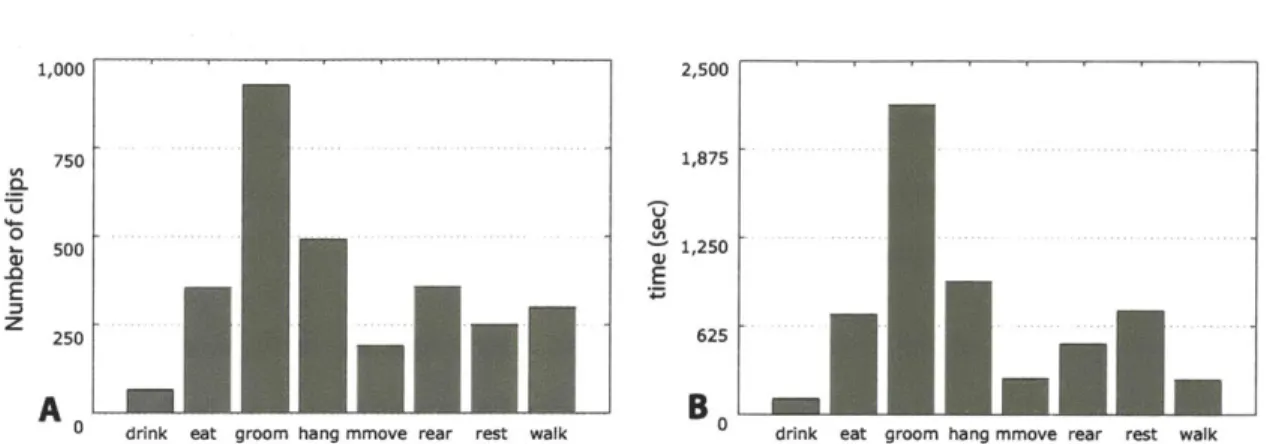
5-2 Distributions of behavior labels for the clipped database over (A) the num-ber of clips and (B) the total time. . . . 91
5-3 Distribution of behavior labels on the (A)full database annotated by 'An-notator group 1' and the (B) set B (a subset of the full database), which was annotated by one more annotator from 'Annotator group 2' (a subset of 'Annotator group 1' ) to evaluate the agreement between two indepen-dent annotators. . . . 91
5-4 Single frames are ambiguous. Each row corresponds to a short video clip. While the leftmost frames (red bounding box) all look quite similar, they each correspond to a different behavior (text on the right side). Because of this ambiguity, frame-based behavior recognition is unreliable and tem-poral models that integrate the local temtem-poral context over adjacent frames are needed for robust behavior recognition. . . . 93
5-5 The number of selected motion templates in each round of the zero-norm SV M . . . 102
5-6 (Top) The accuracy of the system evaluated on the full database and (Bot-tom) the required computation time as a function of the C parameter. . . . . 105
5-7 The accuracy of the system evaluated on thefull database as a function of
length of training video segment. The red cross indicates the performance
of the system when a SVM, instead of SVMHMM, classifier is used. .... 105
5-8 Confusion matrices evaluated on the doubly annotated set B for (A) sys-tem to human scoring, (B) human to human scoring, and (C) CleverSys system to human scoring. Using 'Annotator group 1' as ground truth, the confusion matrices ware obtained for measuring the agreement between the ground truth (row) with the system (computer system), with 'Annotator group 2'(human) and with the baseline software (CleverSys commercial system). For a less cluttered visualization, entry with value less than 0.01 is not shown. The color bar indicates the percent agreement, with more in-tense shades of red indicating agreements close to 100% and lighter shades of blue indicating small fractions of agreement. . . . 107
5-9 Average accuracy of the system for the (A)full database and the (B)
wheel-interaction set as a function of minutes of videos used for training. For each
leave-one-out trial, the system is trained on a representative set of x (x axis of the figure) minutes selected from each training video and tested on the whole length of the left-out video. A representative set consisting of x 1-minute segment is selected to maximize types of actions present in the set. (A) Average accuracy and standard error across the 12 trials, each for one video infull database. (B) Average accuracy and standard error across the
5-10 Average accuracy of the system for the (A)full database and the (B)
wheel-interaction set as a function of minutes of videos used for training. A
representative set of video segments is selected from 0 - 30th min of each
video for training and testing is done on 30th min- end of the same video. A representative set consisting of x (x axis of the figure) 1-minute segment is selected to maximize types of actions present in the set. (A) Average accuracy and standard error across the 12 trials, each for one video in the
full database. (B) Average accuracy and standard error across the 13 trials,
each for one video in the wheel-interaction set. . . . 109
5-11 Confusion matrices evaluated on the doubly annotated set set B for system
to human scoring. Here only motion features are used in the feature com-putation module. For a less cluttered visualization, entry with value less than 0.01 is not shown. The color bar indicates the percent agreement, with more intense shades of red indicating agreements close to 100% and lighter shades of blue indicating small fractions of agreement. . . . 110
5-12 Average time spent for (A) 'hanging' and (B) 'walking' behaviors for each of the four strains of mice over 20 hours. The plots begin at the onset of the dark cycle, which persists for 11 hours (indicated by the gray region), followed by 9 hours of the light cycle. For (A), at every 15 minute of the 20-hour length, we compute the total time one mouse spent for 'hanging' within a one-hour temporal window centering at current time. For (B), the same procedure as in (A) is done for 'walking' behavior. The CAST/EiJ (wild-derived) strain is much more active than the three other strains as measured by their walking and hanging behaviors. Shaded areas corre-spond to 95% confidence intervals and the darker line correcorre-sponds to the mean. The intensity of the colored bars on the top corresponds to the num-ber of strains that exhibit a statistically significant difference (*P;0.01 by ANOVA with Tukey's post test) with the corresponding strain (indicated by
the color of the bar). The intensity of one color is proportional to (N - 1),
where N is the number of groups whose mean is significantly different from the corresponding strain of the color. For example, CAST/EiJ at hour
0 - 7 for walking is significantly higher than the three other strains so N is
3 and the red is the highest intensity. . . . 112
5-13 (A) Snapshots taken from the wheel-interaction set for the four types of interaction behaviors of interest: resting outside of the wheel, awake but not interacting with the wheel, running on the wheel, and interacting with (but not running on) the wheel. (B) Confusion matrices for system to human
sconng. ... ... 116
5-15 Overview of the proposed system for recognizing the home-cage behavior
of mice. The system consists of a feature computation module(A-F) and a classification module(G). (A) The background subtraction technique is performed on each frame to obtain a foreground mask. (B) A bounding box centering at the animal is computed from the foreground mask. (C) Position- and velocity-based features are computed from the foreground mask. (D) Motion-features are computed from the bounding-box within a hierarchical architecture (D-F).(G) HMMSVM. (H) An ethogram of time sequence of labels predicted by the system from a 24-hr continuous record-ing session for one of the CAST/EiJ mice. The right panel shows the ethogram for 24 hours, and the left panel provides a zoom-in version corre-sponding to the first 30 minutes of recording. The animal is highly active as a human experimenter just placed the mouse in a new cage prior to starting the video recording. The animal's behavior alternates between 'walking',
'rearing' and 'hanging' as it explores its new cage. . . . 120
5-16 (A) Average total resting time for each of the four strains of mice over 24 hours. (B) Average duration of resting bouts (defined as a continuous
du-ration with one single label). Mean +/- SEM are shown, *P < 0.01 by
ANOVA with Tukey's post test. (C) Total time spent for grooming exhib-ited by the BTBR strain as compared to the C57BL/6J strain within 10th-20th minute after placing the animals in a novel cage. Mean +/- SEM are
shown, *P < 0.05 by Student's T test, one-tailed. (P = 0.04 for System
and P =0.0254 for human 'H', P =0.0273 for human 'A'). (D-E)
Character-izing the genotype of individual animals based on the patterns of behavior measured by the computer system. (D) Multi-Dimensional Scaling (MDS) analysis performed on the patterns of behaviors computed from the system output over a 24-hour session for the 4 strains. (E) The confusion matrix for the SVM classifier trained on the patterns of behavior using a
6-1 The neuronal tuning properties in the dorsal stream and the effective stimuli. 125 6-2 A. Dynamics of receptive field of directional selective striate simple cells.
Below each contour plot is a ID RF that is obtained by integrating the 2D RF along the yaxis, which is parallel to the cell's preferred orientation. B. Spatiotemporal receptive field for the same cell. The figure is modified from [33]. . . . 126
6-3 The surface indicates the Fourier spectrum of objects translated at a
partic-ular velocity. The slant of the plane from the floor is proportional to the speed of motion. The tile of the plane relative to the spatial frequency axis is equal to the direction of motion. The greater slant of A as compared to B indicate a faster speed in A. The motion in A and C have identical speeds but different directions. Figure modified from [59]. . . . 130 6-4 A. Three patterns moving in different direction produce the same physical
stimulus, as seen through the aperture (Adapted from [115]). B. The object velocity can be decomposed into two orthogonal vectors, one perpendicular to the orientation of the edge and one parallel to the edge. C. . . . 135
6-5 A. An object moves to the right, one if its border (colored in red) appears to
moves up and to the right behind the aperture. B. Each arrow is a velocity vector that generates the percept of the red border in A, and the set of pos-sible velocity vectors lies along a line (colored in red) in the velocity space (Adapted from [115]). C. Each border of the object provides a constraint-a line in velocity spconstraint-ace, constraint-and the intersection of the two lines represent the unique true motion of the object that contains both edges. . . . 136 6-6 Stimulus and direction tuning curve of a hypothetical directional-selective
cell. A. sine wave grating. B. sine wave plaid. C. direction tuning curve to a grating D.ideally predicted direction tuning curve to a plaid, a cell is classified as pattern directional selective if the tuning curve is the same as to the grating (shown in dashed line). A cell is classified as pattern directional selective if the tuning curve is as in bi-lobed solid line. Figure modified from [115] . . . 138
6-7 A zebra in motion. Modified from [110]. . . . .1
6-8 Responses and spectral receptive field of hypothetical cells. (A, B) cells of
separable spatial and temporal frequency tuning. (C, D) cells that are tuned to speed. Figure reprinted from [144] . . . 143 6-9 Construction of MT pattern cell from combination of V1 complex cell
af-ferents, shown in the Fourier domain. Figure reprinted from [177] . . . 144 6-10 Responses of MT cells to (a,d) gratings, (b,e) plaids, and (c,f)
pseudo-plaids. In (a,d), the grating covers one of the two patches within the recep-tive field, as indicated by the stimulus icons. In (b, e), solid curves indicate responses to small plaids with plaid angle 1200. Dashed curves indicate the CDS prediction to the small plaids. The prediction in (b), (e) is obtained from (a), (c), respectively using equation 6.10. In (c, f), solid curves show responses to pseudo-plaids; dashed curves show the CDS prediction based on the two grating tuning curves in (a,d). Reprinted from [97]. . . . 147
6-11 (A) Stimulus (B) Responses of C units to stimuli in (A). Here we
concate-nate responses of C1 units tuned to 16 directions in one plot. The x axis
specifies the preferred direction of each C1 unit. . . . 149
6-12 Responses of ideal S2 units that model MT component and pattern cells. (A)Templates in image space. (B) templates. (C) Directional tuning of templates to gratings (D) Directional tuning of templates to plaids. (E) The pattern sensitivity of the templates. From top to bottom, the templates were "learned" from single grating moving in 0', five superimposed gratings moving in 45', 22.50, 0', 22.5', 45', random dots moving in 0", plaid with
component gratings moving in 45', -45". . . . 150
6-13 Each arrow cluster is a MT subunit where the pattern direction is computed using a WIM model[135]. A MT cell is modeled by the set of nine clusters equally distribute within its receptive filed, and the response is obtained by summing the responses of the 9 clusters. Reprinted from [137]. . . . 151
6-14 Responses of an ideal C2 unit that models MT pattern cells. (A) Stimuli moving in the direction 00. (B) Responses of C1 units to stimuli in (A).
Here we show responses of C1 units tuned to 16 directions and sampled
at 9 locations. (C) Responses of S2 units sampled at 9 locations, all the 9 S2 units store the same template learned from the coherent motion of the
random dots, as shown in 6-12, row 3 , column A. (D) Direction tuning of
the C2 unit to the stimuli moving in 16 directions from 0 to 27r. The C2 unit
computes the maximum responses of the 9 S2 units in (C). (E) R, and Rc
for the C2 unit. . . . 151
6-15 Why normalizing each S2 template's mean . . . 153
6-16 Construction of a speed-tuned MT neuron from VI neurons.(A) Spectral receptive field for three hypothetical VI neurons (B) Spectral receptive
field for a hypothetical MT neuron. Reprinted from [176]. . . . 153
6-17 Snapshots of videos where S2 templates are sampled. (A) Cat Camera. (B)
Street Scenes. (C) HMDB. . . . 154 6-18 Scatter plot of R, and Rc of C2 units. (A) Measured using small plaids.
(B) Measured using pseudo-plaids. . . . 156 6-19 The pattern indices of MT cells measured using pseudo-plaids and small
plaids. Reprinted from [97]. . . . 157
6-20 The pattern indices of C2 units measured using pseudo-plaids and small
plaids. (A) Reprinted from [97]. (B) C2 units with small template sizes.
(C) C2 units with intermediate template sizes. . . . 157
6-21 Suppression index of MT cells and C2 units. (A) Histogram of suppression indices of VI and MT cells. (B) Histogram of suppression indices of C1
and C2 cells. . . . 158
6-22 Histograms of speed tuning indices for DS neurons and model units. (A) speed tuning indices of directional selective neurons VI simple, VI com-plex, and MT neurons, reprinted from [144] (B) speed tuning indices of Si, C1, and C2 units. . . . 160
6-23 Spectral receptive fields for three representative model units.(A) Si unit (B) C1 unit (C) C2 unit. . . . 160
6-24 Scatter plot of R, and Rc of MT neurons and C2 units. (A) [179] (B) [111] (C) 2034 C2 units . . . 161
6-25 What makes a component/pattern cell. (A) R, and Rc plot. (B) Local
sptio-temporal image patches where pattern and component cells are learned. Dotted boxes indicate the synthetic image sequences, and closed boxes in-dicate images from the Cat video as shown in Figure 6-17A. . . . 161
6-26 Some factors that determine the proportion of CDS, PDS, and unclassified
C2 units. (A,C,E) The matching score as a function of video type (A), Si
filter size (C), andS2 template size (E). (B,D,F) The proportion of
compo-nent (blue), unclassified (green), and pattern (red) cells as a function of the
video type(B), the Si filter size (D), and the S2 template size (F). . . . 163
6-27 Some factors that determine the pattern index of C2 units. (A) directional tuning bandwidth vs PI. (B) The proportion of positive coefficients in each
S2 templates vs PI. (C) The proportion of negative coefficients in each S2
tem plates vs PI. . . . 164
6-28 Response of a single cell from the lower bank of monkey STP. The main 8 x 8 grid of traces shows the mean firing rate in response to each specific combination of character and action. Characters are in rows, actions in columns. The actors appeared in a neutral pose at Oms, and began to move at 300ms. Reprinted from [178]. . . . 170
6-29 A comparison between the electrophysiology and model data. Each subplot corresponds to a confusion matrix obtained from ideal data (top row), mon-key data (middle row) and the computational models (bottom row). High probability is indicated by deep red. Stimuli are sorted first by character and then by action. Ideal data (top row) describes the ideal case where the population of cells is tuned to characters (as indicated by 8 x 8 blocks of high probability on the main, left panel); single-pixel diagonal lines of high probability indicate correct classification of actions (right panel). High probability on the main diagonal indicates good performance at pair of character and action. The monkey data is shown in the middle row.
Model data (bottom row), (nj, n2) C2 corresponds to a combination of ni
List of Tables
3.1 Selecting features: System performance for different number of selected
C2 features at rounds 1, 5, 10, 15 and 20 (see text for details). . . . 58
3.2 Comparison between three types of C2 features (gradient based GrC2,
op-tical flow based Of C2 and space-time oriented StC2) and between dense
vs. sparse C2 features. In each column, the number on the left vs. the right
corresponds to the performance of dense [171] vs. sparse [119] C2 features.
Avg is the mean performance across the 4 conditions si, ... s4. Below the performance on each dataset, we indicate the standard error of the mean (s.e.m .). . . . 59
3.3 Comparison between three types of C3 features (gradient based GrC3,
op-tical flow based Of C3 and space-time oriented StC3). In each column,
the number to the left vs. the right corresponds to the performance of C3
features computed from dense [171] vs. sparse [119] C2 features. Avg is
the mean performance across the 4 conditions si,. .. S4. Below the
perfor-mance on each dataset, we indicate the standard error of the mean (s.e.m.). . 60
4.1 Comparison between existing datasets. . . . 69
4.2 Mean recognition performance of low-level shape/color cues for different action databases. . . . 74
4.3 Performance of the benchmark systems on the HMDB51. . . . 77
4.4 Mean recognition performance as a function of camera motion and clip quality. . . . 79
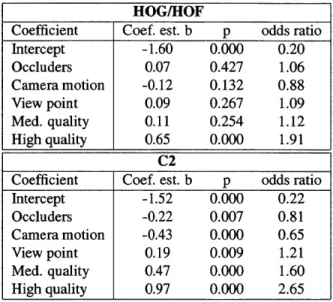
4.5 Results of the logistic regression analysis on the key factors influencing the
performance of the two systems. . . . 80
4.6 Average performance for shape vs. motion cues. . . . 81
5.1 A list of 12 position- and velocity-based features, where V(t) = |C (t)
-Cx(t - 1)|,V(t) = |Cy(t) - Cv(t- 1)|, sV(t) = |Cx(t) - Cx(t - 2)1, and
sfd(t) = (fd(t-2)+fd(t-in)+fd(t)).. 3 ... 97
5.2 7 types of Si types we experimented with and the accuracy evaluated on
the C1 features computed from the 7 types. F is a spatio-temporal filter with size 9 pixels x 9 pixels x 9 frames. X is a space-time patch of the same size. Si(d) is the convolution between the patch X and the F that is
tuned to the d - th direction. . . . 101
5.3 All the video resolutions we experimented with (unit: pixel) and the
accu-racy evaluated on the C1 features. . . . 101
5.4 n, the number of tuned directions of the filters and the accuracy evaluated
on the C 1 features. . . . 101
5.5 The number of selected motion templates in each round of the zero-norm
SVM and the accuracy evaluated on the C2 features. . . . 103
5.6 Accuracy of our system, human annotators and HomeCageScan 2.0
Clever-Sys system evaluated on the set B and thefull database for the recognition
of 8 behaviors. Using 'Annotator group 1' as ground truth, accuracy is computed as percentage of frames correctly classified by a system (chance level is 12.5% for the 8-class classification problem). For the set B, we also report the average of diagonal terms of confusion matrices shown in Figure
5-8, see underlined numbers. . . . 107 5.7 Matching between 8 types of labels in our system and labels in the
HomeCageS-can. . . . 119
6.1 Parameters of SI/Cl units. Here A is set for a preferred speed of 1 pxs/frame. 133
6.2 Tuning properties of S1/Cl units and VI cells . . . 133
6.4 Distribution of R, and Rc of MT cells and C2 units . . . 162
6.5 The parameters of the Poisson model used in [178] and in our experiment. . 171
Chapter 1
Introduction
1.1 The problem
The dorsal stream in the primate visual cortex is involved in the perception of motion and the recognition of actions. The two topics are closely related and have form an important research area crossing the boundaries between several scientific disciplines from computer vision to computational neuroscience and neuropsychology.
Recognizing human actions in videos has also drawn attention in computer vision due to its potential applications in video surveillance, video retrieval/ archival/ compression, and human-computer interaction (Here the term 'action' refers to a meaningful short sequence of motions, such as 'walking', 'running', 'hand-waving', etc). For example, the growing number of images, videos on the internet and movie archives rely on automatic indexing and categorization. In robotics, action recognition is a key to allow the interaction between human and computers and between robots and the environment. In video surveillance, tremendous amount of work of one human observing all the cameras simultaneously can be automated by an action recognition system.
In the field of neuroscience, researchers have been studying how human recognize and understand each other's actions because it plays an important role in the interaction be-tween human and the environment as well as human-human interaction. The brain mech-anisms that are involved in the recognition of actions are believed to be mediated in the
re-sponses are closely related to the perception of motion and behavioral choice [18, 20], and in area STP (superior temporal polysensory area), neurons have been found to be sensitive to whole human body movements such as walking [130], or partial body movements such as mouth-opening/ closing and hand-closing/ opening [216]. Moreover, motion process-ing, the process of inferring the speed and direction of stimulus based on visual inputs, is thought to be highly related to the recognition of actions. Several computational models for motion processing have been built based on neuronal responses to various types of motion [169, 177, 211, 168, 138, 135, 136, 161, 157], and the theoretic solutions have been derived to compute the velocity of an image [64]. These models were able to simulate neurons' se-lectivity to a range of moving patterns but they were not constructed in a system level such that the motion-selectivity could be applied to the recognition of real-world actions.
Action recognition and the motion processing in the visual cortex have been treated as independent problems. In this work, we will bridge the gap of the two problems by building
a dorsal stream model that could explain the physiological recording from neurons in the dorsal stream as well as be used for the recognition of real world actions.
1.2 The approach
The visual information received from retina are processed in two functionally specialized pathways [202, 204]: the ventral stream ('what pathway') that is usually thought of pro-cessing shape and color information and involved in the recognition of objects and faces, and the dorsal stream ('where pathway') that is involved in the space perception, such as measuring the distance to an object or the depth of a scene, and involved in the analysis of motion signals [202, 54], such as perception of motion and recognition of actions. Both streams have the primary visual cortex (Vl) as the source and consist of multiple visual areas beyond V1 (Figure 1-1). Both streams are organized hierarchically in the sense that through a series of processing stages, inputs are transformed into progressively complicated representations while remaining invariant to the change of positions and scales.
Our approach continues two lines of research for the modeling of the visual system. HMAX [152] was based on the organization of the ventral stream and has been applied to
TEMPORAL-*WATr
Figure 1-1: Visual processing in monkeys. Areas in the dorsal stream are shown in green, and areas in the ventral stream are shown in red. Lines connecting the areas indicate known anatomical connections, modified from [201].
the recognition of objects with simple shapes. Its was then extended by Serre et al. for the recognition of complex real-world objects and shown to perform on par with existing computer vision systems [171, 119]. The second line is the model developed by Giese and Poggio [52]. Their model consists of two parallel processing streams, analogous to the ventral and dorsal streams, that are specialized for the analysis of form and optical-flow information, respectively. While their model is successful in explaining physiological data, it has only been tested on simple artificial stimuli such as point-light motion.
1.3 Outline & summary of thesis chapters
The thesis is organized as follows:
Chapter 2 We give an overview of the dorsal stream model that is used throughout the whole thesis work, its physiology origin, and prior related models.
Chapter 3 We introduce the problem of action recognition and describe the use of the model in Chapter 2 as an action recognition system. The performance of the system and the comparison with state of the art computer vision systems are reported on three public action datasets. This chapter was published in 2007 [75].
Chapter 4 While much effort has been devoted to the collection and annotation of large scalable static image datasets containing thousands of image categories, human action datasets lack far behind. In this chapter we present a dataset (HMDB5 1) of 51 human ac-tion categories with a total of around 7,000 clips manually annotated from various sources such as YouTube, HollyWood movies, Google video. We benchmark the performance of low-level features (color and gist) on HMDB51 as well as four previous datasets to show that HMDB51 contains complex motion which can not be easily recognized using simple low-level features. We use this database to evaluate the performance of two representa-tive computer vision systems for action recognition and explore the robustness of these methods under various conditions such as camera motion, viewpoint, video quality and occlusion. This chapter is currently under submission(Kuehne, Jhuang, Garrote, Poggio & Serre, 2011).
Chapter 5 The extensive use of mouse in biology and disease modeling has created a need for high throughput automated behavior analysis tools. In this chapter we extend the action recognition system in Chapter 3 for the recognition of mouse homecage behavior in videos recorded over a 24 hour real lab environment. In addition, two datasets (totally over 20 hours) were collected and annotated frame by frame in order to train the system and evaluate the system's performance. The system was proven to outperform a commercial software and performs on par with human scoring. A range of experiments was also con-ducted to demonstrate the system's performance, its robustness to the environment change, scalability to new complex actions, and its use for the characterization of mice strains. This chapter is published in [73].
Chapter 6 A substantial amount of data about the neural substrates of action recognition is accumulating in neurophysiology, psychophysics and functional imaging, but the un-derlying computational mechanisms remain largely unknown, and it also remains unclear how different experimental evidence is related. Quantitative models will help us organize the data and can be potentially useful for predicting the neuronal tuning for complex hu-man movements in order to understand the representation of movements and how huhu-man recognize actions. In this chapter, we show that the model in Chapter 2 could explain
neu-rophysiology of the dorsal stream -it not only mimics the organization of the dorsal stream,
but the outputs of the model could also simulate the neuronal responses along the dorsal hierarchy. Specifically, the model account for the spatiotemporal frequency selectivity of V1 cells, pattern and component sensitivity and distribution [161], local motion integration [97], and speed-tuning [144] of MT cells. The model, when combining with the ventral stream model [173], could also explain the action and actor selectivity in the STP area, a high level cortical area receiving inputs from both the ventral and the dorsal stream. An early version of this chapter is published in [74].
1.4 Contribution
Chapter 3 Recognition of actions has drawn attention for its potential applications in computer vision and the role in social interactions that has intrigued neuroscientists. Com-puter vision algorithms for the recognition of actions and models for the motion processing in the dorsal stream have been developed independently. Indeed, none of the existing neu-robiological models of motion processing have been used on real-world data [52, 24, 175]. As recent works in object recognition have indicated, models of cortical processing are starting to suggest new algorithms for the computer vision [171, 119, 148]. Our main
con-tribution for this topic is to connect the two lines of work, action recognition and motion processing in the dorsal stream, by building a biologically plausible system with the orga-nization of the dorsal stream and apply it to the recognition of real world actions. In order
to extend the neurobiological model for object recognition [171] into a model for action recognition, we mainly modify it in the following ways:
* Propose and experiment with different types of motion-sensitive units. " Experiment with the dense and sparse features proposed in [119].
* Experiment with the effect of the number of features on the model's performance. " Experiment with the technique of feature selection.
* Add two stages to the model to account for the sequence-selectivity of neurons in the dorsal stream.
" Evaluate the system's performance on three publicly available datasets.
* Compare the system's performance with a state-of-the-art computer vision system.
Chapter 4 The proposed HMDB database is, to our knowledge, the largest and perhaps the most realistic available database to-date. Each clip of the database was validated by at least two human observers to ensure consistency. Additional meta-information allows a precise selection of test data as well as training and evaluation of recognition systems. The meta tags for each clip include the camera view-point, presence or absence of camera motion and occluders, and the video quality, as well as the number of actors involved in the action. This should allow for the design of more flexible experiments to test the perfor-mance of state-of-the-art computer vision databases using selected subsets of this database.
Our main contribution is the collection of the dataset HMDB51 and perform various ex-periments to demonstrate that it is more challanging than existing action datasets. Our
specific contribution are:
* Compare the performance of low-level features (color and gist) on HMDB51 as well as four previous datasets.
* Compare the performance of two representative systems on HMDB51: C2 features
[75] and HOG/HOF features [86].
" Evaluate the robustness of two benchmark systems to various sources of image degra-dations.
" Discuss the relative role of shape vs. . motion information for action recognition.
" Using the metadata associated with each clip in the database to study the influence
of variation (camera motion, position, occlusions, etc. ) on the performance of the
two benchmark systems.
Chapter 5 Existing sensor-based and tracking-based approaches are successfully applied to the analysis of coarse locomotion such as active vs. resting, or global behavioral states such as distance traveled by an animal or its speed. However these global measurements limit the complexity of the behaviors that can be analyzed. The limitation of sensor-based approach can be complemented by vision-based approaches. Indeed two vision-based sys-tems have been developed for the recognition of mice behaviors [36, 218, 219]. However, these systems haven't been tested in a real-world lab setting using long uninterrupted video sequences containing potentially ambiguous behaviors or at least evaluated against human manual annotations on large databases of video sequences using different animals and dif-ferent recording sessions. Our main contribution is to successfully apply a vision-based
action recognition system to the recognition of mice behaviors, to test the system on a huge dataset that includes multiple mice under different recording sessions, and to compare the performance of the system with that of human annotators and the commercial software (CleverSys, Inc). Our specific contributions are:
* Datasets. Currently, the only public dataset for mouse behavior is limited in scope: it contains 435 clips and 6 types of actions [36]. In order to train and test our system on a real-world lab setting where mice behaviors are continuously observed and scored over hours or even days, we collect two types of datasets: clipped database andfull
database.
- The clipped database contains 4, 200 clips with the most exemplary instances
of each behavior (joint work with Andrew Steele and Estibaliz Garrote).
- Thefull database consists of 12 videos, in which each frame is annotated (joint
- The SetB: a subset offull database, in which each frame has a second annotation
(joint work with Andrew Steele).
- Make above datasets available.
* Feature computation stage
- Optimizing motion-sensitive units by experimenting with the number of tuned
directions, different types of normalization of features and video resolutions.
- Learning a dictionary of motion patterns from the clipped dataset.
- Designing a set of position features that helps the recognition of context-dependent
actions.
- Implementing the computation of motion features using GPU (based on CNS
written by Jim Mutch [118]).
" Classification stage
- Experimenting with two different machine learning approaches (SVM vs. SVMHMM).
- Optimizing the parameters of SVMHMM.
- Experimenting with the number of required training examples for the system to
reach a good performance. * Evaluation
- Comparing the accuracy of the system with a commercial software and with
human scoring.
- Demonstrating the system's robustness to partial occlusions of mice that arose
from the bedding at the bottom of homecage.
- Demonstrating the system is indeed trainable by training it to recognize the
interaction of mice with a wheel. * Large-scale phenotypic analysis
- Building a statistical model based on the system's predictions to 28 animal of 4 strains in a home-cage environment over 24 hours, and showing that the statis-tical model is able to characterize the 4 strains with an accuracy of 90%.
- Based on system's predictions, we can reproduce the results of a previous
exper-iment that discovered the difference of grooming behaviors between 2 strains of mice.
Chapter 6 The motion processing in the dorsal stream has been studied since 80's [64,
177, 138, 161, 136, 137, 198, 197, 157, 58]. The existing models could explain a range of known neuronal properties along the dorsal hierarchy. These models are however in-complete for three reasons. First, they are not constructed to be applicable in read world tasks. Second, most of them couldn't explain the neural properties beyond the first two stages (VI and MT) of the dorsal hierarchy. Third, they couldn't explain the recent results of neurophysiology [144, 97]. Our main contribution is to use the model proposed for
ac-tion recogniac-tion to explain the dorsal stream qualitatively and quantitatively by comparing outputs of model units with neuronal responses to stimuli with various types of complexity and motion. Our specific contributions are:
" A detailed survey for the known neuronal properties along the dorsal stream.
" Design a population of spatiotemporal filters to match the statistics of VI cells [47]. * Simulate the pattern and component sensitivity of MT cells [115].
" Simulate the continuous distribution of pattern and component sensitivity of MT cells [161].
" Propose the origin of continuous pattern and component sensitivity MT cells. " Simulate the speed tuned VI complex and MT cells [144].
" Simulate the motion opponency of MT cells [180].
Chapter 2
The Model
In this chapter, we describe the dorsal stream model that will be used in the next three chapters for various tasks from computer vision to neurophysiology.
2.1 Motivation from physiology
The receptive field (RF) of a cell in the visual system is defined as the region of retina over which one can influence the firing of that cell. In the early 1960s, David Hubel and Torsten Wiesel mapped the receptive field structures of single cells from the primary visual cortex of cat and monkey [68, 69] using bright slits and edges. They concluded that a majority of cortical cells respond to edges of a particular orientation, and cells could be grouped into "simple" or "complex" cells, depending on the complexity of the receptive field structures. Simple receptive field contains oriented excitatory regions in which presenting an edge stimulus excited the cell and inhibitory regions in which stimulus presentation suppressed responses. Hubel and Wiesel suggested simple cells structures could be shaped by receiving inputs from several lateral geniculate cells arranged along an oriented line, as shown in Figure 2-1.
Complex receptive fields differ from the simple fields in that they respond with sus-tained firing over substantial regions, usually the entire receptive field, instead of over a very narrow boundary separating excitatory and inhibitory regions. Most of the complex cells also have larger receptive field size than simple cells. Hubel and Wiesel suggested
Figure 2-1: A possible scheme for explaining the elongated subfields of simple receptive field. Reprinted from [69].
Figure 2-2: A possible
Reprinted from [69].
scheme for explaining the organization of complex receptive fields.
complex cells pool the response of a number of simple cells whose receptive field is lo-cated closely in space, therefore the activation of any simple cell can drive the repones of the complex cell, as shown in Figure 2-2.
Moving edges are more effective in eliciting responses of orientation selective cells than stationary edges. Some cells show similar responses to the two opposite directions perpendicular to the preferred orientation, and the rest of the cells are direction selective, meaning cells show a clear preference of moving direction. Directional selective V1 cells
distribute in the upper layer 4 (4a, 4b, and 4Ca) and layer 6 of the visual cortex [62].
These cells then project to area MT [203], where most of neurons are direction and speed I
sensitive and the receptive field is 2 - 3 times larger than V1 direction selective neurons [107]. MT neurons then project to MST, where neurons are tuned to complex optical-flow patterns over a large portion of the visual field, and are invariant to the position of moving
stimulus [56]. The linked pathway of visual area V1, MT, and MST is called dorsal steam
("where" pathway) and is thought to be specialized for the analysis of visual motion. Non-direction selective VI cells distribute in the layer 2, 3, and 4 (4C3) of the visual cortex. They project to cortical areas V2, to V4, and then to the inferiortemporal area (IT). IT cells respond selectively to highly complex stimuli (such as faces) and also invari-antly over several degrees of visual angle. This pathway is called ventral stream ("what" pathway) and is thought to be specialized for the analysis of object shape.
It was hypothesized that the two streams form functionally distinct but parallel pro-cessing pathways for visual signals. Their computations are similar in the sense that lower level simple features are gradually transformed into higher level complex features when one goes along the visual streams [202].
2.2
Background: hierarchical models for object
recogni-tion
The recognition of objects is a fundamental, frequently performed cognition task with two fundamental requirements: selectivity and invariance. For example, we can recognize a specific face despite changes in viewpoint, scale, illumination or expression. V1 simple and complex cells seem to provide a good base for the two requirements. As a visual signal passes from LGN to V1 simple cells, its representation increases in selectivity; only pat-terns of oriented edges are represented. As the signal passes from V1 simple to complex cells the representation gains invariance to spatial transformation. Complex cells down-stream from simple cells that respond only when their preferred feature appears in a small window of space now represent stimuli presented over a larger region.
Motivated by the finding of Hubel and Wiesel, several models have been proposed to arrange simple and complex units in a hierarchical network for the recognition of objects or
digits. In these models, simple units selectively represent features from inputs, and complex units allow for the positional positional errors in the features. The series of work starts with the Neocognitron model proposed by Fukushima [49], followed by the convolutional network by Lecun [88], and then HMAX by Riesenhuber & Poggio [152].
The early version of HMAX uses a limited handcrafted dictionary of features in inter-mediate stages and is therefore too simple to deal with real-world objects of complex shape. In its more recent version developed by Serre et al. [173], a large dictionary of intermediate features are learned from natural images and the trained model is able to recognize objects from cluttered scene or from a large number of object categories. HMAX could also ex-plain neurobiology: the computations in HMAX were shown to be biologically plausible circuits and outputs of different layers could simulate the neuronal responses in the area V1, V4, and IT [172, 80]. A sketch of HMAX is shown in Figure 2-3.
0S
,.(2 1) S \ 2
~00 AJ~
View-tuned cells
Complex composite cells (C2)
Composite feature cells (S2) -- I
Complex cells (C1)
Simple cells (S1)
- weighted sum
-MAX
Figure 2-3: HMAX. Figure reprinted from [152] ... a
2.3
The model
The problem of action recognition could be treated as a three-dimensional object recogni-tion problem, in which selectivity to particular morecogni-tion patterns (as a combinarecogni-tion of direc-tion and speed) and invariance to the visual appearance of the subjects play an important role for the recognition of particular action categories. Here we propose a model for the recognition of actions based on HMAX. Our model is also a hierarchy; where simple and complex layers are arranged repetitively to gradually gain the specificity and invariance
of input features. The main difference from HMAX is, instead of representing oriented edge features from stationary stimuli, our model represents motion features (directional and speed) of stimuli. Our model is also different from HMAX in terms of detailed imple-mentations, such as normalization of features.
Here we describe an overview of the model structure and a typical implementation. The detailed implementation will vary depending on the particular task and will be described in each of the subsequent chapters. The model's general form is a hierarchy of 4 layers
Si -* C1 -> S2 -+ C2: 2 simple layers, Si and S2, and 2 complex layers, C1 and C2.
Features are selectively represented in the S(simple) layer using a template matching op-eration. Features are invariantly represented accordingly in the C(complex) layer using a
max pooling operation. The model is illustrated in Figure 2-4. The first two stages (S1,
C1) are designed to mimic the receptive field structures of Vl simple and complex cells,
respectively. The latter two stages (S2,C2) are designed to repeat the computations in the
first two stages. S2 and C2 units are our prediction to neurons in the higher-level cortical
areas. We will verify this prediction in Chapter 5.
2.3.1
S
1The input to the model is a gray-value video sequence that is first analyzed by an array of Si units at all spatial and temporal positions. A Si unit is a three-dimensional filter (two in space and one in time), such as Gabor filter, tuned to a combination of motion (direction and speed) in a particular spatial and temporal scale. Here scale refers to the spatial and temporal size of the filter. Let I denote the light intensity distribution of a stimulus, f
tlP3
S2 ~~1 Template matching or weighted sum MAXFigure 2-4: The structure of the proposed model. The model consists of a hierarchy of layers with template matching operations (S layer) and max pooling operations (C layer). The two types of operations increase the selectivity and invariance to position and scale change.
denote a receptive field of a Si unit. The linear response is computed as the convolution of the stimulus with the unit:
f .1
(2.1)
||fI|
x|I|1|
The absolute value is then taken to make features invariant to contrast reversal. For the recognition of actions in a video with frame rate 25 fps, we typically use 8 Gabor filters tuned to 4 directions and 2 speeds. For a typical video resolution 240 x 320 (pixels), we use one single scale representation, and filter size 9 (pixels) x 9 (pixels) x 9 (frames).
2.3.2
C1
At the next step of processing, at each point of time(frame), C1 units pool over a set of Si units distributed in a local spatial region by computing the single maximum response
over the outputs of Si units with the same selectivity (e.g. same preferred direction and speed). To avoid over-representation of motion feature caused by continuously pooling from adjacent spatial regions, the max-pooling is not performed at all the locations. Assume each C1 unit pools over a spatial n x n (pixel) grid, we only use C1 units at every n/2 pixel locations. If multiple scales of Si units are used, a C1 unit computes the max response in both neighboring spatial positions and across scales. As a result a Cl unit will have a preferred velocity as its input Si units but will respond more tolerantly to small shifts in the stimulus position and scale.
2.3.3 S
2The S2 stage detects motion features with intermediate complexity by performing a
tem-plate matching between inputs with a set of temtem-plates(prototypes) extracted during a train-ing phase. The template matchtrain-ing is performed at each position and each scale of the C1 outputs. A template is defined as a collection of responses of spatially neighboring C1 units that are tuned to all possible selectivity at a particular scale. Each template is computed from a small spatio-temporal patch randomly sampled from training videos. One can think
that a template corresponds to the weights of a S2 unit, and the preferred feature of the S2
unit is the template. The responses of a S2 unit to an input video can be thought of as the
similarity of the stimulus' motion (C1 encoded) to previously seen motion patterns encoded in the same layer (C1).
Let ni denote the number of S1
/C
1 selectivity (i.e. the number of tuned directions x thenumber of tuned speeds) and ne the number of spatially neighboring C1 units converging
into a S2 unit, a template's size is ne (pixels) x nc (pixels) x n, (types). A template
with large spatial size (nc) includes features from a large region and therefore has higher
complexity in the feature space than a small template. In the task of action recognition, templates with many sizes are used to encode motion of a range of complexity. A set of
typical values is ne = 4, 8, 12, 16 (pixels).
The S2 units compute normalized dot product (linear kernel); let w denote the unit's
![Figure reprinted from [9] . . . . . . . . . . . . . . . . . . . . . . . . . . . 48 3-2 Local space-time interest points detected from a space-time shape of a](https://thumb-eu.123doks.com/thumbv2/123doknet/14752971.581066/11.918.137.776.428.1087/figure-reprinted-local-space-points-detected-space-shape.webp)