HAL Id: hal-02470280
https://hal.umontpellier.fr/hal-02470280
Submitted on 9 Mar 2020
HAL is a multi-disciplinary open access
archive for the deposit and dissemination of
sci-entific research documents, whether they are
pub-lished or not. The documents may come from
teaching and research institutions in France or
abroad, or from public or private research centers.
L’archive ouverte pluridisciplinaire HAL, est
destinée au dépôt et à la diffusion de documents
scientifiques de niveau recherche, publiés ou non,
émanant des établissements d’enseignement et de
recherche français ou étrangers, des laboratoires
publics ou privés.
Distributed under a Creative Commons Attribution - NonCommercial - NoDerivatives| 4.0
based on deep learning
Sue Han Lee, Hervé Goëau, Pierre Bonnet, Alexis Joly
To cite this version:
Sue Han Lee, Hervé Goëau, Pierre Bonnet, Alexis Joly. New perspectives on plant disease
charac-terization based on deep learning. Computers and Electronics in Agriculture, Elsevier, 2020, 170,
pp.105220. �10.1016/j.compag.2020.105220�. �hal-02470280�
Contents lists available atScienceDirect
Computers and Electronics in Agriculture
journal homepage:www.elsevier.com/locate/compagNew perspectives on plant disease characterization based on deep learning
Sue Han Lee
a,⁎, Hervé Goëau
a,b, Pierre Bonnet
a,b, Alexis Joly
c aAMAP, Univ Montpellier, CIRAD, CNRS, INRA, IRD, Montpellier, FrancebCIRAD, UMR AMAP, Montpellier, France
cINRIA Sophia-Antipolis – ZENITH team, LIRMM, Montpellier, France
A R T I C L E I N F O Keywords:
Plant diseases
Automated visual crops analysis Deep learning
Transfer learning
A B S T R A C T
The control of plant diseases is a major challenge to ensure global food security and sustainable agriculture. Several recent studies have proposed to improve existing procedures for early detection of plant diseases through modern automatic image recognition systems based on deep learning. In this article, we study these methods in detail, especially those based on convolutional neural networks. We first examine whether it is more relevant to fine-tune a pre-trained model on a plant identification task rather than a general object recognition task. In particular, we show, through visualization techniques, that the characteristics learned differ according to the approach adopted and that they do not necessarily focus on the part affected by the disease. Therefore, we introduce a more intuitive method that considers diseases independently of crops, and we show that it is more effective than the classic crop-disease pair approach, especially when dealing with disease involving crops that are not illustrated in the training database. This finding therefore encourages future research to rethink the current de facto paradigm of crop disease categorization.
1. Introduction
A plant disease is an alteration of the original state of the plant that affects or modifies its vital functions. It is mainly caused by bacteria, fungi, microscopic animals or viruses, and has a strong impact on agricultural yields and on farm budget. According to the Food and Agriculture Organization of the United Nations, transboundary plant diseases have increased significantly in recent years due to globaliza-tion, trade, climate change and the reduction in the resilience of pro-duction systems due to decades of agricultural intensification. The risk of transboundary epidemics is increasing and can cause huge losses in crops, threatening the livelihoods of vulnerable farmers and the food and nutritional security of millions of people.1Early detection of dis-ease symptoms is one of the main challenges in protecting crops and limiting epidemics. Initial disease identification is usually done by vi-sual assessment (Barbedo, 2016) and the quality of the diagnosis de-pends heavily on the knowledge of human experts (Liu et al., 2017). However, human expertise is not easily acquired by all actors of the agricultural world, and is less accessible, especially in the case of small farms in developing countries.
Automatic recognition of plant diseases by image analysis re-presents a promising solution to overcome this problem and reduce the lack of expertise in this field (Ramcharan et al., 2017). Several studies
have been carried out on isolated crops, such as maize (Wiesner-Hanks et al., 2018), cassava (Ramcharan et al., 2017), tomato (Fuentes et al., 2017; Durmus et al., 2017; Fuentes et al., 2018), apple (Liu et al., 2017), wheat (Johannes et al., 2017; Picon et al., 2018), citrus (Iqbal et al., 2018) or potato (Oppenheim and Shani, 2017). Deep Learning (DL) techniques, including Convolutional Neural Networks (CNN), have emerged as the most promising approaches given their ability to learn reliable and discriminative visual characteristics. Tranfer learning, which is used in most cases (Slado Jevic et al., 2016; Too et al., 2019; Fuentes et al., 2017; Liu et al., 2017; Mohanty et al., 2016; Ramcharan et al., 2017), is not a single technique, but a whole family of methods, comprising, among others those commonly known as fine-tuning. Un-like learning from scratch where the weights of a model are learned from scratch, the weights of a pre-trained model on a large general dataset (in terms of number of images and classes, such as ImageNet) are fine-tuned. Transfer learning allows to build accurate models even on a specialized dataset such as those containing plant diseases where there are usually a small number of images and classes compared to ImageNet. Indeed, when used to training a CNN model based on images of diseased and healthy plant leaves captured under controlled condi-tions, it has been proven that fine-tuning is better than training a deep model from scratch (Mohanty et al., 2016). However, the ability of a deep learning model to transfer knowledge from one domain to
https://doi.org/10.1016/j.compag.2020.105220
Received 11 January 2019; Received in revised form 24 December 2019; Accepted 8 January 2020
⁎Corresponding author.
E-mail addresses:[email protected](S.H. Lee),[email protected](H. Goëau),[email protected](P. Bonnet),[email protected](A. Joly).
1http://www.fao.org/emergencies/emergency-types/plant-pests-and-diseases/en/.
Available online 06 February 2020
0168-1699/ © 2020 The Authors. Published by Elsevier B.V. This is an open access article under the CC BY-NC-ND license (http://creativecommons.org/licenses/BY-NC-ND/4.0/).
another, from one task to another, is not yet well understood and performances may vary according to the used datasets for pre-training a model (Torralba and Efros, 2011). In particular, (Zhou et al., 2014) showed that fine-tuning a CNN pre-trained on scene recognition data-sets rather than the general Imagenet dataset can perform better in any urban scene recognition tasks. We can then assume that a model pre-trained on a dataset of images dedicated to plant identification could provide better features for plant disease identification rather than a pre-trained model on ImageNet which contains actually few visual bota-nical concepts. However, no previous study has reported such results. The first contribution of this article is to study the impact of transfer learning depending on whether the transfer learning is from a general domain or from the plant domain.
In recent years, more and more studies address the multi-crop dis-ease problems where data modelling covers several varieties of crops and diseases at the same time (Mohanty et al., 2016; Too et al., 2019; Slado Jevic et al., 2016; Ferentinos, 2018). These investigations cor-respond to the needs of actors such as farm technicians, agricultural engineers, market gardeners or arboriculturists, who would potentially be confronted with different types of diseases on different types of crops, and where a more general approach (particularly through the use of smartphones) could provide a valuable help (Mohanty et al., 2016). From a technological point of view, this type of use is now possible thanks to deep learning techniques that prove to have sufficiently high recognition capabilities for wide datasets in terms of number of images, thus avoiding the need to design hand-crafted features dedicated to a specific domain. To date, two main datasets have been used to assess identification performance on multi-crop diseases: Plant Village (PV)2 (Hughes and Salathé, 2015) and Digipathos3(Barbedo et al., 2018). The majority of studies are based on the PV dataset (Slado Jevic et al., 2016; Ferentinos, 2018; Mohanty et al., 2016; Hughes and Salathé, 2015), which is currently the largest dataset in terms of number of images. The PV dataset is organized into target classes where each one represents a crop-disease pair, i.e. an association of one type of crop and one disease. In the PV dataset, a particular crop may be present in several classes and, conversely, visually similar diseases with the same disease common name may be present in several classes. Most of the previous studies based on CNNs follow this data organization, where the last layer dedicated to the classification contains output of crop-disease pairs (Mohanty et al., 2016; Too et al., 2019; Slado Jevic et al., 2016; Ferentinos, 2018).
However, although previous studies have reported high identifica-tion performances, it is possible that the models learned are not optimal by extracting to many irrelevant features related more to crop than to disease. For example, as reported in (Mohanty et al., 2016), it has been proven that removing the background with image segmentation is less effective than using the ordinary colored background images to train a CNN, confirming a dependency of background features for disease identification. Furthermore, (Toda and Okura, 2019) showed that model which is supposed to learn plant disease visual appearance, tends to highlight irrelevant crop features like the shape of the leaf, and in fact, it is possible when a crop contains more visual discrimination characteristics than the disease itself such as a deeply grooved leaf of tomato. Therefore, the second contribution of this paper is to propose a new intuitive way of characterizing plant diseases in the context of multi-crop diseases, focusing on the common names of diseases re-gardless of the type of crop. We show that this approach is more gen-eralizable and robust in identifying diseases of new data taken in do-mains different from those in the training set.
Next, we consider that it would be very difficult, if not impossible, in a real-world application to collect a complete set of images illus-trating each crop-disease pair. Also, it may not be easy to establish a
specific list of all diseases for each host species. We note that pathogens with a wide host range can infect many different host species. For ex-ample, as reported in (Prospero and Cleary, 2017), nearly 200 plant species can be infected with bacterial wilt (Ralstonia solanacearum). Therefore, the ability of a model to transfer knowledge from one disease context to another is crucial for practical application to reduce the time and cost of data collection and retraining a deep model. We show that by using our new strategy mentioned above to identify plant diseases, we could have the significant advantage of being able to identify a disease known to the classifier without the type of crop being known. Therefore, the third contribution of this paper is to study the general-ization of a deep model to identify diseases of “unseen” crops. Unseen crops in this context refer to unknown crops that have never been seen by a deep model during the training.
To summarize the contributions of this paper:
1. We investigate the impact of two transfer learning strategies, one based on a pre-trained model on a plant dataset and the other using a general object dataset. We found that, it is sometimes more ef-fective to fine-tune a model pre-trained on plant identification, or one which is pre-trained on general object recognition.
2. We qualitatively investigate the features learned from the models trained with crop-disease classes (Mohanty et al., 2016; Too et al., 2018). We highlight that the learned features might not necessarily be relevant to plant disease identification because they also focus on crop-specific features such as the leaf venation and lamina. 3. We demonstrate a simple and intuitive way of considering plant
diseases alone, without any association with a crop. With this, it shown to enable a better generalization not only to new data taken in domains different from those in the training (different in data distribution), but also to unseen crops.
2. Datasets 2.1. Plant Village
Plant Village (PV) (Hughes and Salathé, 2015) is a popular dataset collected for evaluation of automatic plant disease identification sys-tems. It contains healthy and infected leaves isolated on a uniform background. We used the initial version of the PV dataset2that is still
publicly available as a benchmark in this study. It has 38 crop-disease pairs, with 26 crop-disease categories for 14 crop plants. Note that, the data comes with predefined training and test subsets. In our study, we use the reported configuration as the one that produces the best iden-tification performances in the original document (Mohanty et al., 2016), where 80% of the data is for the training set and the remaining 20% for the test (more precisely, 43,810 training images and 10,495 images for the test).Table 1gives for the 38 pairs, the common names of the host plant and the disease, the scientific name of the disease and the number of training and testing images.
We can see in this table that different crops can be infected with pathogens associated with the same common disease name. It is mainly due to their similar ways of infecting the crops, which hence has led the agricultural community to call them by the same name.Table 2 illus-trates the distribution of images based on a total of 14 crops and 20 common diseases4with 1 healthy class. Some diseases such as Apple scab or Tomato mosaic virus can only be found in apple and tomato crops respectively, but other diseases such as Black rot or Bacterial spot are common in different crops.
2https://github.com/spMohanty/PlantVillage-Dataset. 3https://www.digipathos-rep.cnptia.embrapa.br/.
4common names of plant diseases that have been recommended based on
2.2. IPM and Bing test datasets
Two complementary datasets named IPM and Bing, which were initially introduced in (Mohanty et al., 2016), are used in this work to evaluate the robustness of a model for predicting plant diseases on exterior images. Unlike in PV, these test images are not limited to a controlled environment (seeFig. 1) and are extracted from a reliable online sources for IPM5and downloaded from Bing Image Search. These images were verified in (Mohanty et al., 2016). We were able to retrieve all the 119 images from IPM6mentioned in (Mohanty et al., 2016), but we could only retrieve 64 of the 121 images expected for Bing6(missing
images are no longer available online).Tables 3 and 4show the dis-tribution of the IPM and Bing images. Among the 38 crop-disease pairs in PV, the IPM test set allows to evaluate 19 pairs while Bing test set allows to evaluate 26 pairs. A qualitative assessment of the data, as shown inFig. 1, shows that Bing images contain background noise (i.e. cluttered backgrounds) more often than IPM image, suggesting a more difficult recognition on Bing than on IPM.
3. Transfer learning and pre-trained models
Transfer learning is not a single technique, but a whole family of methods, comprising, among others those commonly known as fine-tuning. Using such approaches, a model trained on a task is re-purposed
to a second related task (Goodfellow et al., 2016). A basic example of transfer learning is using a deep model just as fixed feature extractor (Karpathy, 2019), without tuning the weights of a pre-trained model and by removing the last fully connected layer related to the class outputs of the initial task. Then any learning algorithms such as sup-port-vector machines can be used to perform new classification. One of the most popular transfer learning approaches is to fine-tune all the weights of a pre-trained model, with the last fully connected layer being replaced and randomly initialized on a new classification task. In fact, it is possible to fine-tune only some layers, which are generally the last layers corresponding to a higher level of abstraction. However, (Yosinski et al., 2014) showed that by transferring the features and fine-tuning all the layers of a network, one can boost the generalization capability of a model. Fine-tuning helps to prevent overfitting, leading to significantly better generalization especially when the number of labelled examples is scarce, or in a transfer setting where we have lots of examples for some source tasks but very few for some target tasks (LeCun et al., 2015). Additionally, it has been proven to be more ef-fective if the pre-training and the target task are correlated (Yosinski et al., 2014; Huh et al., 1608).
In plant disease classification tasks, it has been shown that the transfer learning approach is more accurate than a “from scratch” learning approach where all the weights of a model are learned from scratch (Too et al., 2018; Mohanty et al., 2016; Slado Jevic et al., 2016; Ferentinos, 2018). Most of these previous works are based on models pre-trained on ImageNet (Russakovsky et al., 2015), a general image database containing about 1,2 million images associated to 1000 very diverse classes (animals, vehicles, buildings, landscapes, plants, etc).
Table 1
Description of the PV dataset. Note that (%) is the percentage per class.
Class Plant common name Disease common name Disease scientific name Train (%) Test (%) C1 Apple Apple scab Venturia inaequalis 498 1.14 132 1.26 C2 Apple Black rot Diplodia seriata 484 1.10 137 1.31 C3 Apple Cedar apple rust Gymnosporangium juniperi-virginianae 220 0.50 55 0.52
C4 Apple Healthy – 1336 30.5 309 2.94
C5 Blueberry Healthy – 1231 2.81 271 2.58
C6 Cherry (including sour) Powdery mildew Podosphaera clandestina 948 2.16 104 0.99 C7 Cherry (including sour) Healthy – 703 1.60 151 1.44 C8 Corn (maize) Cercospora leaf spot Gray leaf spot Cercospora zeae-maydis 409 0.93 104 0.99 C9 Corn (maize) Common rust Puccinia sorghi 954 2.18 238 2.27 C10 Corn (maize) Northern Leaf Blight Setosphaeria turcica 798 1.82 187 1.78
C11 Corn (maize) Healthy – 934 2.13 228 2.17
C12 Grape Black rot Guignardia bidwellii 884 2.02 296 2.82 C13 Grape Esca (Black Measles) Togninia minima 1099 2.51 284 2.71 C14 Grape Leaf blight (Isariopsis Leaf Spot) Pseudocercospora vitis 828 1.89 248 2.36
C15 Grape Healthy – 341 0.78 82 0.78
C16 Orange Haunglongbing (Citrus greening) Liberibacter asiaticus 4361 9.95 1146 10.92 C17 Peach Bacterial spot Xanthomonas arboricola 1819 4.15 478 4.55
C18 Peach Healthy – 280 0.64 80 0.76
C19 Pepper bell Bacteria spot Xanthomonas campestris 781 1.78 216 2.06
C20 Pepper bell Healthy – 1267 2.89 211 2.01
C21 Potato Early blight Alternaria solani 824 1.88 176 1.68 C22 Potato Late blight Phytophthora infestans 768 1.75 232 2.21
C23 Potato Healthy – 116 0.26 36 0.34
C24 Raspberry Healthy – 208 0.47 163 1.55
C25 Soybean Healthy – 4202 9.59 888 8.46
C26 Squash Powdery mildew Podosphaera xanthii (including Erysiphe cichoracearum) 1503 3.43 332 3.16 C27 Strawberry Leaf scorch Diplocarpon earlianum 931 2.13 178 1.70
C28 Strawberry Healthy – 388 0.89 68 0.65
C29 Tomato Bacteria spot Xanthomonas campestris 1739 3.97 388 3.70 C30 Tomato Early blight Alternaria solani 839 1.92 161 1.53 C31 Tomato Late blight Phytophthora infestans 1560 3.56 349 3.33 C32 Tomato Leaf mold Mycovellosiella fulva 768 1.75 184 1.75 C33 Tomato Septoria leaf spot Septoria lycopersici 1456 3.32 315 3.00 C34 Tomato Spider mites Two-spotted spider mite Tetranychidae spp. 1312 2.99 364 3.47 C35 Tomato Target Spot Corynespora cassiicola 1136 2.59 268 2.55 C36 Tomato Tomato Yellow Leaf Curl Virus TYLCV 4312 9.84 1045 9.96 C37 Tomato Tomato mosaic virus ToMV 307 0.70 66 0.63
C38 Tomato Healthy – 1266 2.89 325 3.10
Total 43,810 100 10,495 100
5https://images.bugwood.org/.
Table 2 Distribution of diseases for different types of crops. Note that, (%) is the percentage of images per row/column. Healthy Apple scab Black rot Cedar apple rust Powdery mildew Cercospora leaf spot Gray leaf spot Common rust Northern leaf blight Esca (Black Measles) Leaf blight (Isariopsis Leaf Spot) Haunglong- bing (Citrus greening) Bacterial spot Apple 1645 630 621 275 Blueberry 1502 Cherry 854 1052 Corn 1162 513 1192 985 Grape 423 1180 1383 1076 Orange 5507 Peach 360 2297 Pepper bell 1478 997 Potato 152 Raspberry 371 Soybean 5090 Squash 1835 Strawberry 456 Tomato 1591 2127 Total 15,084 630 1801 275 2887 513 1192 985 1383 1076 5507 5421 (%) 27.78 1.16 3.32 0.51 5.32 0.94 2.20 1.81 2.55 1.98 10.14 9.98 Early blight Late blight Leaf scorch Leaf Mold Septoria leaf spot Spider mites Two-spotted spider mite Target Spot Tomato Yellow Leaf Curl Virus Tomato mosaic virus Total (%) Apple 3171 5.84 Blueberry 1502 2.77 Cherry 1906 3.51 Corn 3852 7.09 Grape 4062 7.48 Orange 5507 10.14 Peach 2657 4.89 Pepper bell 2475 4.56 Potato 1000 1000 2152 3.96 Raspberry 371 0.68 Soybean 5090 9.37 Squash 1835 3.38 Strawberry 1109 1565 2.88 Tomato 1000 1909 952 1771 1676 1404 5357 373 18,160 33.44 Total 2000 2909 1109 952 1771 1676 1404 5357 373 54,305 100 (%) 3.68 5.36 2.04 1.75 3.26 3.09 2.59 9.86 0.69 100
However, in the case of plant diseases, one can suppose that it would be appropriate to pre-train a model on domain with a dataset containing exclusively plant images. Therefore, in this study, we compare two fine-tuning strategies, one directly using a model pre-trained on ImageNet and another one using PlantCLEF2015, a dataset dedicated to plant identification (H. Go¨eau, P. Bonnet, A. Joly, Lifeclef plant identifica-tion task, 2015). This dataset is related to the plant identification challenge in LifeCLEF (Joly et al., 2015) and addresses the problem of species identification based on multi-organ and multi-image observa-tions of specimens. It has the same number of classes as ImageNet, but is two orders of magnitude smaller with precisely 91,759 training images (seeFig. 2for some illustrations).
4. Identification based on common names of diseases and generalization to unseen crops
4.1. Identification based on visual features of common diseases
With regard to previous works on crop-disease pairs (Mohanty et al., 2016; Ferentinos, 2018), there remains a doubt that a deep model can be forced to discriminate similar diseases that have the same common name and most likely visually similar ways of infecting the crops. A potentially undesirable effect that may occur is that the model learns more from the content related to the crop than the visual content re-lated to the disease (Toda and Okura, 2019; Mohanty et al., 2016). This
adverse effect can potentially be amplified if a crop has a very pro-nounced characteristic such as toothed margins leaves, while the dis-ease is not very visible, for example, with a slight bleaching at an early stage of infection. In this section, we study an alternative approach to the usual crop-disease pair modeling by considering only on common names of diseases regardless of crop categories. The hypothesis is that such intuitive modelling will engage the model to learn more in-dependent features from the host plants.
In order to train a disease classifier based on common diseases in-dependently of crops, the images of the PV dataset are first separated into 21 classes (20 diseases and one healthy class). We randomly took a subset of images (~20%) from each healthy crop and combined them
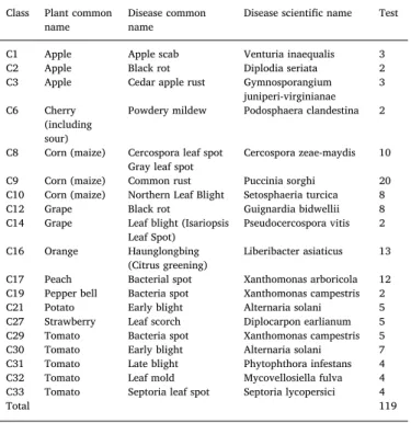
Fig. 1. Examples of the (a) IPM and (b) Bing images. Table 3
Description of the IPM images.
Class Plant common
name Disease commonname Disease scientific name Test C1 Apple Apple scab Venturia inaequalis 3 C2 Apple Black rot Diplodia seriata 2 C3 Apple Cedar apple rust Gymnosporangium
juniperi-virginianae 3 C6 Cherry
(including sour)
Powdery mildew Podosphaera clandestina 2 C8 Corn (maize) Cercospora leaf spot
Gray leaf spot Cercospora zeae-maydis 10 C9 Corn (maize) Common rust Puccinia sorghi 20 C10 Corn (maize) Northern Leaf Blight Setosphaeria turcica 8 C12 Grape Black rot Guignardia bidwellii 8 C14 Grape Leaf blight (Isariopsis
Leaf Spot) Pseudocercospora vitis 2 C16 Orange Haunglongbing
(Citrus greening) Liberibacter asiaticus 13 C17 Peach Bacterial spot Xanthomonas arboricola 12 C19 Pepper bell Bacteria spot Xanthomonas campestris 2 C21 Potato Early blight Alternaria solani 5 C27 Strawberry Leaf scorch Diplocarpon earlianum 5 C29 Tomato Bacteria spot Xanthomonas campestris 5 C30 Tomato Early blight Alternaria solani 7 C31 Tomato Late blight Phytophthora infestans 4 C32 Tomato Leaf mold Mycovellosiella fulva 4 C33 Tomato Septoria leaf spot Septoria lycopersici 4
Total 119
Table 4
Description of the Bing images.
Class Plant common
name Disease commonname Disease scientific name Test C1 Apple Apple scab Venturia inaequalis 6 C2 Apple Black rot Diplodia seriata 3 C3 Apple Cedar apple rust Gymnosporangium
juniperi-virginianae 3 C4 Apple Healthy – 1 C7 Cherry (including sour) Healthy – 1
C8 Corn (maize) Cercospora leaf spot
Gray leaf spot Cercospora zeae-maydis 3 C9 Corn (maize) Common rust Puccinia sorghi 3 C10 Corn (maize) Northern Leaf Blight Setosphaeria turcica 1 C11 Corn (maize) Healthy – 2 C14 Grape Leaf blight (Isariopsis
Leaf Spot) Pseudocercospora vitis 1 C16 Orange Haunglongbing
(Citrus greening) Liberibacter asiaticus 3
C18 Peach Healthy – 1
C19 Pepper bell Bacteria spot Xanthomonas campestris 1 C21 Potato Early blight Alternaria solani 1 C22 Potato Late blight Phytophthora infestans 3 C24 Raspberry Healthy – 1 C28 Strawberry Healthy – 2 C29 Tomato Bacteria spot Xanthomonas campestris 1 C30 Tomato Early blight Alternaria solani 3 C31 Tomato Late blight Phytophthora infestans 3 C32 Tomato Leaf mold Mycovellosiella fulva 6 C33 Tomato Septoria leaf spot Septoria lycopersici 3 C34 Tomato Spider mites
Two-spotted spider mite Tetranychidae spp. 1 C35 Tomato Target Spot Corynespora cassiicola 6 C36 Tomato Tomato Yellow Leaf
Curl Virus TYLCV 1
C38 Tomato Healthy – 4
Total 64
Fig. 2. Examples of the PlantCLEF2015 images. The images are composed of
different plant organs, and captured in environment with cluttered back-grounds, reflecting a realworld scenario.
into a single healthy class, so as to limit the amount to 2601 images in order to avoid imbalanced distributions (39,508 training images in total). During the inference, we calculate the classification result from the 21 probability outputs produced by the trained model. We call this disease modeling strategy Sco which symbolizes the CNN modeling strategy based on the common name of diseases.
We compare Scowith another disease modeling strategy calledScd, which instantiates the CNN modeling strategy based on the crop-disease pairs. InScd, we first train a CNN based on 38 crop-disease pairs with a total of 43,810 training images. During the inference, from the 38 probability outputs produced by the trained model, we perform a late fusion method to integrate the probabilities corresponding to the in-dividual common diseases. More precisely, we compute the average probability output with respect to each individual common name of disease for the conjoined crop-disease pairs. For example, the average probability of the Back rot common disease which is associated with apple and grape, is computed as:
=
PBlackrot mean P( Apple Black rot__ _ ,PGrape Black rot__ _ )
With this formulation,Scdhas the same number of accuracy outputs as Sco.
4.2. Generalization to unseen crops
There are several hundred common plant diseases in the world that can each of them potentially infect dozens or even hundreds of different types of crops. It is difficult, if not impossible, to collect a complete set of images illustrating each crop-disease combination for building an exhaustive training set. In addition, diseases can mutate and become transmissible to new cultivated species and then it is necessary to complete regularly the training set with new crop-disease combina-tions. On the other hand, an approach that considers diseases in-dependently of crops has the advantage of making a classifier more easily extensible to new crops, by allowing a model to identify a known disease in the training dataset, even if the crop hosting the diseases on a test image is unknown in the training dataset. To evaluate the ability of a deep model to generalize to an unknown crop, in our methodology, all the images related to pepper crops such as those from the class Pepper_bell__Bacterial_spot and the class Pepper_bell__healthy are removed from the training set, and the model is trained only with those images which are not from pepper crop. It should be noted that, in doing so, the number of crop-disease pairs to be learned by a model is reduced from 38 to 36, giving a total of 41,762 and 37,727 images in the training set to trainScdand Scorespectively.
5. Approach 5.1. Deep architectures
In our study, we employ three types of CNN architectures with different depth size: VGG16 (Simonyan and Zisserman, 1409) (16 layers), InceptionV3 (Szegedy et al., 2016) (48 layers) and our proposed architecture GoogLeNetBN7 (34 layers). This last architecture is in-spired by the InceptionV2 and InceptionV3 architectures (Ioffe and Szegedy, 2015; Szegedy et al., 2016) that bring several upgrades to the initial GoogLeNet architecture (Szegedy et al., 2014) for increasing the accuracy and reducing the computational complexity. It is a 34 layers deep CNN adding to each convolution a batch normalization (BN) op-eration. BN has been proven to speed up convergence and limit over-fitting. Besides applying BN to GoogLeNet, we update the network by replacing the 5 × 5 convolutional layers with two consecutive layers of 3x3 convolutions like for the InceptionV3 architecture, so as to improve computational speed. The ImageNet dataset used for the ILSVRC
challenge (Russakovsky et al., 2015), containing about 1.2 M images related to 1000 classes, was then used to train the model from scratch for a few days on a mini-cluster of GPU cards to produce a “pre-trained” model.
5.2. Training from scratch versus transfer learning
All CNNs are trained by using stochastic gradient descent (SGD) optimization technique. The batch size was set to 45, and momentum set to 0.9. The L2 weight decay with penalty multiplier was set to
×
2 10 4. By employing the CNNs mentioned in Section 5.1 and training
them based on the following training schemes, we will have 9 trained models based on 3 experimental configurations:
1. Transfer learning
(a) Fine-tuning of ImageNet pre-trained model (FTIN) (b) Fine-tuning of PlantCLEF2015 pre-trained model (FTPC) 2. Training from scratch (FS)
For the FTIN configuration, a model is first pre-trained with ImageNet and then fine-tuned directly on the PV dataset. For the FTPC configuration, a model is first pre-trained with ImageNet, then fine-tuned on the PlantCLEF2015 dataset before being fine-fine-tuned on the PV dataset. For both configurations, all weights of the pre-trained models are fine-tuned simultaneously, with the last fully connected layer being replaced and initialized with target task classes. All the choices of training hyper-parameters were made based on empirical observation of the convergence of the network training as well as the training performance. For the two architectures VGG16 and GoogLeNetBN, the learning rate was initially set with a relatively low value of 10 4in order
to change the weights not too quickly, except for the last full-connected layer where the learning rate was set to a higher value of10 3to
ac-celerate the convergence of the weights initialized with random values. For each model, the training are carried out for a total of 15 epochs, where one epoch is defined as the number of iterations required for the neural network to pass through the entire training set. The learning rate followed a “step” policy, meaning that it is decreased by a factor of 10 during the training, for every 15/3 epochs in our case. The architecture InceptionV3 with the configuration FTPC used the same hyper-para-meters as the aforementioned two architectures, but when using the configuration FTIN on ImageNet the initial learning rate was set to10 3
for all the layers because we noticed that the model converged too slowly with a low initial learning rate of 10 4. For the FS configuration,
we set for all the three models an initial learning rate of10 3for all the
layers. In this case, since all the weights are initialized with random values, we need more iterations, 30 epochs in these experiments, for the models to converge towards their best performances. Concerning the inputs, during the training, the image at the input of GoogLeNetBN and VGG16 is resized to 256×256 pixels and cropped to 224×224 pixels. As with InceptionV3, the image is resized to 300 × 300 pixels and cropped to 299 × 299 pixels. We augment our training image by random cropping and mirroring. For final model evaluations, each test image is cropped in its center and resized to the size imposed by the model architecture.
Fig. 3shows the progression of the top-1 accuracy on the training set for all the different models and configurations limited to 15 epochs. We can see that the models learned with a fine-tuning approach all progress very quickly and tend to achieve a top-1 accuracy above 0.95 in less than 2 epochs, except for the InceptionV3 model pre-trained on ImageNet, which requires at least 7 epochs to reach an equivalent ac-curacy. We can also see that, in the FS configuration, the models con-verge more slowly and requires at least 11 epochs before reaching ac-curacies equivalent to the transfer learning configurations, except for the model with the VGG16 architecture which seems to stagnate around
an accuracy of 0.91.
6. Experiments
In this section, we first studied the impact of the use of transfer learning on the identification of plant diseases. Then, we evaluated a new classification problem considering common names of diseases as single classes, regardless of crop categories. Finally, we studied and analyzed the extent to which the deep models we learned can be gen-eralizable to diseases despite the fact that the hosting crop is not illu-strated in the training set.
6.1. Comparison of models with different learning configurations Evaluation measures on the test sets. To measure model classifica-tion performance, the top-1 and top-3 accuracies were used to measure the performance of model classification in our experiments. Further, we also used the average accuracy per class to assess the performance of an individual class:AVE=C1 iC=1Ti, whereTi is the average accuracy for all test images related to the Ciclass and C is the total number of classes. Next, to overcome the stochasticity of learning a single neural network, we used the same approach as described in (Mohanty et al., 2016), which combines the predictions of several trained models. Specifically, we aggregated and calculated the average of all the probabilities given
by the models saved at the end of each epoch, then we calculated the average and overall accuracy of the entire test. By doing so, we are able to reduce the variance of the prediction results and obtain a fair com-parison result with (Mohanty et al., 2016).
Generalization.Table 5shows the classification performance of the CNNs trained with the different learning strategies. It can be seen that, although models trained with FS configuration, especially the deeper architectures, achieve relatively high performance in PV test set, they have lower classification performance in IPM and Bing than fine-tuned models. This result is consistent with the previous study (Mohanty et al., 2016), showing the advantage of fine-tuning in this task. The GoogLeNet model (Mohanty et al., 2016), which achieves the highest accuracy on the PV test set, shows lower performance on IPM images compared to GoogLeNetBN. This leads us to conclude that this model is particularly overfitted. Unlike what is generally observed in many other areas, the VGG16 model achieves the best performance on IPM and Bing test sets, 44.54% and 28.13% respectively, surpassing deeper chitectures. This finding suggests that those models with deeper ar-chitectures are more likely to be overfitting for this task, probably be-cause the PV dataset is not large or diverse enough.
Pre-trained models. It is difficult to conclude which pre-training task works best for the external IPM and Bing test data mainly because the size of these two set of images is quite small. However, by comparing the overall top-1 accuracy of the combined IPM and Bing images, the
Fig. 3. Progression of top-1 accuracy on the training set for the 3 models and the 3 configurations.
Table 5
Classification results of CNNs trained with 3 different training configurations: fine-tuning on ImageNet trained CNN (FTIN), fine-tuning on PlantCLEF2015 pre-trained CNN (FTPC) and training from scratch (FS). It shows the top-1 and top-3 accuracy (%) and the average accuracy per class AVE (%) for all the test sets.
2*Architecture 2*Configuration PV test set IPM images Bing images
top-1 top-3 AVE top-1 top-3 AVE top-1 top-3 AVE
GoogLeNetBN FTIN 98.22 99.80 97.51 39.50 63.87 32.98 17.19 39.06 23.08
FTPC 99.09 99.95 98.83 42.86 62.18 39.85 23.44 43.75 26.92
FS 98.21 99.80 97.40 20.17 45.38 19.95 10.94 21.88 10.26 VGG16 (Simonyan and Zisserman, 1409) FTIN 99.00 99.93 98.61 44.54 67.23 45.95 26.56 46.88 26.92 FTPC 98.56 99.90 97.84 36.13 64.71 35.43 28.13 43.75 33.97
FS 91.97 98.47 88.10 15.97 24.37 16.85 6.25 10.94 6.41 InceptionV3 (Szegedy et al., 2016) FTIN 98.33 99.82 97.47 26.89 53.78 36.70 15.63 34.38 21.14
FTPC 98.46 99.89 97.71 37.82 65.55 34.36 23.44 45.31 27.56
FS 99.31 99.81 99.01 21.01 37.82 17.83 10.94 18.75 10.26
VGG16 pre-trained with the ImageNet dataset shows a better result than the one pre-trained with PlantCLEF2015, which are 44.54% and 36.13% respectively. As for the GoogLeNetBN and InceptionV3, the model pre-trained on PlantCLEF2015 leads to better performance than the one pre-trained on the ImageNet dataset, unlike the VGG16. From this observation, it is unfortunately not possible to conclude on the usefulness or not of pre-training the models on a task closer to the target domain rather than the general object dataset, ImageNet.
Confusions and misclassifications. By analyzing the performance
of each individual class of the PV test set (Supplementary Fig. 1), we found that most classification errors occur in the Tomato Early blight class. A closer analysis of the confusion matrix (Supplementary Table 1–6) shows that these errors generally result from confusion be-tween the classes Tomato Early blight, Tomato Late blight, Tomato Septoria leaf spot and Tomato Target spot. Fig. 4gives some examples of mis-classified images related to these confusions and illustrates how they visually share similarities in leaf appearance and disease patterns. Al-though the disease Tomato Early blight may have specific visual char-acteristics, the intra- and inter-class variability makes their learning very difficult. This factor was discussed in (Barbedo, 2018), and one suggested solution was to extend the training dataset to a more ex-haustive and complete set, covering all the visual variability of symp-toms, which is in fact very difficult to collect. Next, we found that misclassification tends to occur within similar crops, particularly in maize and potatoes, and is also misleading due to visually similar leaf appearance and disease patterns.
Next, by analyzing the performance of the Bing images (Supplementary Table 7-12), we observed that with the exception of the VGG16 model pre-trained on PlantCLEF2015 (Supplementary Table 10), which has the correct prediction for all the images of Potato Late blight, the rest of the model configurations show major classifica-tion errors, confusing these images with Tomato Late blight, which is actually related to the same common name of disease but on different crops. This observation suggests that a common disease, although in-fecting different host types, produces very similar disease patterns. 6.1.1. Qualitative results
Attention map visualization. To better understand the visual fea-tures learned by the models, we used one of the visualization methods presented in (Yosinski et al., 2015), which consists of plotting the ac-tivation values of neurons in a CNN layer in response to an input image. Instead of individually visualizing the activation of a CNN layer as implemented in (Mohanty et al., 2016), we examined the highest global activation within all feature maps in a layer, so as to locate the regions most voted by the model and then exploit those that have the most impact in the final classification. More precisely, we started by plotting the position of the neuron with the highest activation for all the features maps extracted from the last convolutional layer, and from there we accumulated the first 30 dominant activations and matched them to the original image. It is possible to visualize any number of neural activa-tions, but, based on our empirical observation, the accumulation of 30
dominant activations in this case is enough to visualize the difference in the focus of attention between different models. We chose to visualize the last convolutional layer because this layer corresponded to the highest level of abstraction and it is more specific to the target classes (Lee et al., 2017; Zeiler et al., 2011).
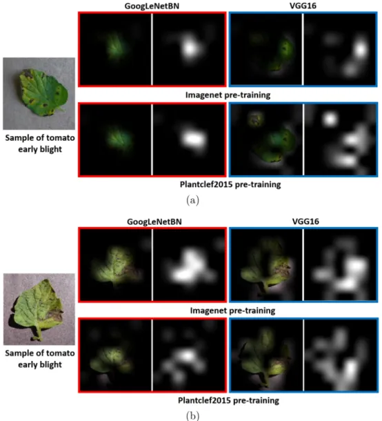
By comparing the visualization outputs of the GoogLeNetBN and VGG16, we found that their neuron activations were activated in dif-ferent regions. For example, inFig. 5a, both the GoogLeNetBN models pre-trained with ImageNet and PlantCLEF2015 are activated by areas of yellowish venation, while the VGG16 models are activated by areas infected with large brown spots with yellow tissues around. However, when comparing the visualization outputs of different pre-training tasks on the same network architecture, we found a certain degree of simi-larity in the activated areas. For example, inFig. 5b, the GoogLeNetBN models pre-trained with ImageNet and PlantCLEF2015 concentrate mainly on the center of the leaf, while the VGG16 models mostly focus on infected secondary veins. On closer observation, we found that the activated regions do not necessarily focus on the largest infected area, but on regions with obvious leaf characteristics such as the venations. 6.1.2. Discussion
In connection to the above findings, we hereby make a few deduc-tions. Firstly, we found that VGG achieves a better classification per-formance compared to other deeper network architectures which tend to overfit on the PV dataset. We believe that the lack of diversity in the PV data set, which could make the learned model sometimes misleading when used in real field data such as IPM and Bing. Secondly, it is not possible to conclude that a model pre-trained on a task closer to the final task is the best option to solve the PV dataset, as in our study we found that pre-training on plant domains improves performance in the case of deep networks, InceptionV3 and GoogLeNetBN, but not for the simpler and shallower networks such as VGG16. However, in our ex-periments, the generalization performances of the models were studied on IPM and Bing, which is currently the only field test set available online with verified field truth. It would be interesting to see if our results hold up on a larger number of images. If not, it might suggest that the size of the IPM and Bing is too small to generalize the results. Further investigation of the complementary field datasets will be re-quired to reach a more robust conclusion on this point. We hope that this article will stimulate the curiosity of the scientific community in this field and facilitate further research on this topic related to the generalization of the deep model in cross domains to improve the identification of plant diseases.
Lastly, we noticed that the features learned might not necessarily look at the most obviously infected area but the region with the most distinctive leaf characteristics, such as the venation. This is believed to be due to the fact that models are trained with the terminology of crop-disease pairs, where models trained in this way could be biased towards crop-specific patterns, especially when crop features appear to be more discriminative than diseases. Therefore, in the next section, we explore an alternative approach to crop-disease modelling, attempting an
Fig. 4. Examples of leaf samples which are confused between classes of: (a) Tomato Early blight and Tomato Late blight, and (b) Tomato Early blight and Tomato
intuitive way to direct a deep model to learn feature representations based on common diseases, regardless of crop.
6.2. Disease identification based on common names of diseases and generalization to unseen crops
In this experiment we used the VGG16 model, which had been proven to be the best model in previous experiments, to experiment with the principle of learning based on common names of diseases. We compared two disease modeling strategies that are: (1) the formation of a model based on training solely on the common names of diseases (Sco), and (2) based on training on previously proposed crop-disease target classes and the subsequent implementation of a late fusion method to integrate probabilities corresponding to the individual common names of diseases (Scd). Details of these approaches can be found in section 4. 6.2.1. Evaluation on seen crops
Table 6shows that theScdapproach is generally better than the Sco approach at predicting the PV (seen) set. The VGG16 model pre-trained with ImageNet gives the best result up to 98.98% top-1 accuracy and 98.20% average accuracy per class AVE. However, due to the nature of the PV data set, which seriously lacks diversity, both strategies were
found achieving a relatively high accuracy (:98% for top-1 accuracy). Through the analysis of the confusion matrices (Supplementary table 19–20) of the ScoandScdapproaches, we found that, compared toScd, Sco has more classification errors between early blight and late blight. In fact, this misclassification occurs mainly in tomato crops where the number of disease classes is highest in PV. From this observation, we deduce that the lack of crop information may seem to affect Sco's ability to recognize diseases with a very similar visual appearance. However, we note that although crop characteristics that could be extracted byScd may provide additional information to help differentiate these classes, these crop characteristics do not necessarily correspond to the char-acteristics of plant diseases.
Next, we analyzed the performance of deep models to identify new data (IPM and Bing) from other domains, typically pictures in the field. Note that there are only two pepper crop images in IPM, and one pepper crop image in Bing, of which the number of samples is insufficient to infer the performance of deep models in recognizing the disease of an unseen crop. We hence tested the deep model using only the seen crop images. FromTable 6, we can see that Sco approach in general works better thanScdon IPM and Bing. Next, using the Scoapproach, in order to determine which pre-training task is the most effective, we compared the top-1 accuracy of the combined IPM and Bing images, and found
Fig. 5. Visualization of the attention maps of the GoogLeNetBN and VGG16 for the PV sample. The upper and lower row images are the output visualization of the
that with ImageNet pre-training can achieve the highest top-1 classifi-cation performance, i.e. 45%, while the PlantCLEF2015 pre-training is 42.22%.
6.2.2. Generalization to unseen crops
FromTable 6, we can see that, despite the fact thatScdcan achieve a better result in the PV (seen) set, Scogeneralizes better to PV (unseen) set, especially the PlantCLEF2015 model which reaches 65.11%, the highest top-1 accuracy. Note that the overall accuracy of the PV (un-seen) in Table 6was calculated from all PV (unseen) images, which means a combination of images from the Pepper_bell__Bacterial_spot and Pepper_bell__healthy classes. Next, we explored the classification perfor-mance of each individual PV (unseen) class in which, in this case, the overall accuracy is calculated according to each individual PV (unseen) class. The result of the classification is presented inTable 7.
We observed that different pre-training tasks can exert substantial influence on different categories of pepper classes. Specifically, it can be seen that, for the Sco, the ImageNet pre-trained model (83.89%) can distinguish better between healthy and unhealthy pepper leaf samples compared to that pre-trained with PlantCLEF2015 (65.40%). However, the class of pepper leaves with bacteria spots shows a contrary result where the model pre-trained with the PlantCLEF2015 (65.75%) is better than the one pre-trained with the ImageNet (43.06%).
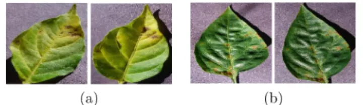
Next, based on failure analysis of the PV (unseen), we observed that, with the ImageNet pre-trained models, a majority of Pepper bell Bacterial spot are confused with target spot, Huanglongbing (Citrus greening) and early blight; with the PlantCLEF2015 pre-trained models, most of the Pepper bell Bacterial spot images are confused with Haunglongbing (Citrus greening), Tomato Yellow Leaf Curl Virus and early blight. Through visual analysis, we noticed that the symptoms of those mis-classified samples are very similar to the disease from the other class. For example, inFig. 6a, the samples of Pepper bell Bacterial spot that are confused with Haunglongbing (Citrus greening) have yellowish infected regions and also yellow veins, resembling the characteristics of Haun-glongbing (Citrus greening). Also, those samples that are confused with the Target spot disease as shown inFig. 6b have visually similar dark brown spots characteristics. Likewise, the healthy pepper samples are also found to be misled for the same reason. A majority of pepper healthy samples are wrongly identified as Haunglongbing (Citrus
greening), most probably due to the characteristic of yellowing pepper bell leaves.
From this analysis, it is obvious that the recognition of deep models is highly affected by the symptom variations of one disease, analogous to the findings reported in (Barbedo, 2018). However, it is undeniable that, for the models formulated by bothScdand Scothat have never seen any pepper bell leaf samples, they are still able to capture very similar characteristics of pepper bell which could somehow help to improve the predictive modeling for unseen crops.
Lastly, by aggregating multi-class outputs into two classes, we ana-lyzed the performance of the models to differentiate between healthy and unhealthy classes of the PV set. Note that, in this experiment, we verified the classification performance on the basis of the entire PV set, which includes the seen and unseen test set. From the ROC (Receiver Operating Characteristic) curves shown inSupplementary Fig. 2, it can be seen that the Sco is more robust in differentiating between healthy and unhealthy leaf samples compared to the model trained withScd. Indeed, through the AUC (Area Under the Curve) as shown inTable 8, Sco as a whole per-formed better thanScd.
6.2.3. Discussion
Based on this experiment, we make several deductions. Firstly, classification based on Scowas proven generalizes better and robust in identifying diseases of unseen crops as well as plant images taken in domains different from those in the training set. Next, Scocan also better distinguish between healthy and unhealthy leaf samples. This is parti-cularly important in the context of phenotyping large field crops, in which it is possible with new agricultural robots or drones to generate
Table 6
Performance of the VGG16 models on the disease classification problem based on Scoand Scd. Note that the performance of IPM and Bing is based on only seen crop
images while the unseen crop refers to Pepper_bellBacterial_spot and Pepper_bellhealthy.
Pretrained dataset PV (seen) (%) PV (unseen) (%) IPM images (%) Bing images (%)
(Scd/Sco) top-1 top-3 AVE top-1 top-3 top-1 top-3 AVE top-1 top-3 AVE
ImageNet (Sco) 98.94 99.96 98.19 63.23 90.87 46.15 76.92 52.29 42.86 63.49 34.31
ImageNet (Scd) 98.98 99.96 98.20 34.89 79.86 45.30 74.36 48.54 39.68 61.90 35.78
PlantCLEF2015 (Sco) 98.42 99.91 97.31 65.11 90.87 48.72 79.49 52.29 30.16 58.73 29.90
PlantCLEF2015 (Scd) 98.52 99.86 97.70 37.47 81.97 43.59 73.50 44.92 26.98 47.62 26.47
Table 7
Results of the individual classification of diseases related to the pepper bell crop for the PV (unseen). It presents the top-1 accuracy of the Pepper_bellBacterial_spot and Pepper_bellhealthy for the Scoand Scdwith different
pre-training tasks.
Pepper class ImageNet PlantCLEF2015
Sco Scd Sco Scd
bacteria spot 43.06 18.98 65.74 42.59 healthy 83.89 51.18 65.40 32.23
Fig. 6. Examples of pepper bell leaves that are confused with (a)
Haunglongbing (Citrus greening) and (b) Target spot disease.
Table 8
Performance of the VGG16 models on the healthy and unhealthy classification of the PV set.
Pretraining task Classifier AUC
ImageNet Sco 0.972
Scd 0.744
PlantCLEF2015 Sco 0.967
massive volumes of visual data that can't be manually exhaustively analyzed. In such cases, an early detection of unhealthy leaf samples can contribute to quickly investigate their origins, and potentially im-plement appropriate solutions.
7. Conclusion
First, this paper has examined and compared the performance of different transfer learning mechanisms based on different (1) pre-training tasks: the plant specialized domain and general object domain, and the (2) network architectures: VGG16 (16 layers), GoogLeNetBN (34 layers) and InceptionV3 (48 layers). We have experimentally proven that pre-training with plant specialized tasks could reduce the impact of overfitting for the deeper Inception-based model but the VGG16 model with ImageNet pre-training has shown a better generalization in adapting to new data.
Second, the fact that the VGG16 perform better than the inception-based models would be due to the lack of diversity in the PV data set, which leads to a constraint in the deployment of deeper architectures. Nevertheless, with regard to the fact that ImageNet pre-training does not necessarily regularize or improve the accuracy of final target tasks, as indicated in (He et al., 1811), we suggest that the agricultural community move forward to create a broader and more diversified plant disease database, without having to use a pre-training model. In addition, for the model to better adapt to large-scale crops, a dataset of images captured under real cultivation conditions (Barbedo, 2018; Ferentinos, 2018) is needed, as demonstrated by (Ferentinos, 2018).
Third, by interpreting the underlying learned characteristics through the visualization of activations, we have showed that a CNN trained in this crop-disease terminology may not always focus on dis-ease regions but crop-specific characteristics such as leaf venation or lamination to facilitate data discrimination. Therefore, in order to capture the visual symptoms of plant diseases, we demonstrated an intuitive way of leading a deep model to learn the representation of characteristics based on the common names of diseases instead of target classes of crop-disease pairs. We have shown experimentally that the model trained with common diseases, regardless of crop is more gen-eralizable, especially for new data taken in different domains and also for unseen crops.
CRediT authorship contribution statement
Sue Han Lee: Conceptualization, Methodology, Software,
Validation, Formal analysis, Investigation, Visualization, Resources, Data curation, Writing - original draft. Hervé Goëau: Formal analysis, Investigation, Conceptualization, Methodology, Writing - review & editing, Visualization. Pierre Bonnet: Formal analysis, Investigation, Supervision, Project administration, Funding acquisition, Resources, Data curation, Writing - review & editing. Alexis Joly: Formal analysis, Investigation, Conceptualization, Methodology, Supervision, Project administration, Funding acquisition, Writing - review & editing.
Declaration of Competing Interest
The authors declare that they have no known competing financial interests or personal relationships that could have appeared to influ-ence the work reported in this paper.
Acknowledgement
This project is supported by Agropolis Fondation, Numev, Cemeb, #DigitAG, under the reference ID 1604-019 through the < < Investissements davenir > > programme (Labex Agro:ANR-10-LABX-0001-01).
Appendix A. Supplementary material
Supplementary data to this article can be found online athttps:// doi.org/10.1016/j.compag.2020.105220.
References
Barbedo, J.G.A., 2016. A review on the main challenges in automatic plant disease identification based on visible range images. Biosyst. Eng. 144, 52–60.
Barbedo, J.G.A., 2018. Impact of dataset size and variety on the effectiveness of deep learning and transfer learning for plant disease classification. Comput. Electron. Agric. 153, 46–53.
Barbedo, J.G., 2018. Factors influencing the use of deep learning for plant disease re-cognition. Biosyst. Eng. 172, 84–91.
Barbedo, J.G.A., Koenigkan, L.V., Halfeld-Vieira, B.A., Costa, R.V., Nechet, K.L., Godoy, C.V., Junior, M.L., Patricio, F.R.A., Talamini, V., Chitarra, L.G., et al., 2018. Annotated plant pathology databases for image-based detection and recognition of diseases. IEEE Lat. Am. Trans. 16, 1749–1757.
Durmus, H., Gune, E.O., Kırcı, s.M., 2017. Disease detection on the leaves of the tomato plants by using deep learning. In: Agro-Geoinformatics, 2017 6th International Conference on, IEEE, 2017, pp. 1–5.
Ferentinos, K.P., 2018. Deep learning models for plant disease detection and diagnosis. Comput. Electron. Agric. 145, 311–318.
Fuentes, A., Yoon, S., Kim, S.C., Park, D.S., 2017. A robust deep-learning based detector for real-time tomato plant diseases and pests recognition. Sensors 17, 2022.
Fuentes, A.F., Yoon, S., Lee, J., Park, D.S., 2018. High-performance deep neural network-based tomato plant diseases and pests diagnosis system with refinement filter bank. Front. Plant Sci. 9.
Goeau, H., Bonnet, P., Joly, A., 2015. Lifeclef plant identification task 2015. In: Working Notes of CLEF 2015 – Conference and Labs of the Evaluation forum, Toulouse, France, September 8-11, 2015, 2015. URL: http://ceur-ws.org/Vol-1391/157-CR.pdf.
Goodfellow, I., Bengio, Y., Courville, A., 2016. Deep learning (adaptive computation and machine learning series). Adapt. Computat. Mach. Learn. Series 800.
K. He, R. Girshick, P. Dollar, Rethinking imagenet pre-training, arXiv preprint arXiv:1811. 08883 (2018).
D. Hughes, M. Salathe, et al., An open access repository of images on plant health to enable the development of mobile disease diagnostics, arXiv preprint arXiv:1511. 08060 (2015).
M. Huh, P. Agrawal, A.A. Efros, What makes imagenet good for transfer learning? arXiv preprint arXiv:1608.08614 (2016).
S. Ioffe, C. Szegedy, Batch normalization: Accelerating deep network training by reducing internal covariate shift, CoRR abs/1502.03167 (2015). URL: http://arxiv.org/abs/ 1502.03167. arXiv:1502.03167.
Iqbal, Z., Khan, M.A., Sharif, M., Shah, J.H., Ur Rehman, M.H., Javed, K., 2018. An au-tomated detection and classification of citrus plant diseases using image processing techniques: a review. Comput. Electron. Agric. 153, 12–32.
Johannes, A., Picon, A., Alvarez-Gila, A., Echazarra, J., Rodriguez Vaamonde, S., Nava Jas, A.D., Ortiz-Barredo, A., 2017. Automatic plant disease diagnosis using mobile capture devices, applied on a wheat use case. Comput. Electron. Agric. 138, 200–209. Joly, A., Goeau, H., Glotin, H., Spampinato, C., Bonnet, P., Vellinga, W.-P., Planque, R., Rauber, A., Palazzo, S., Fisher, B., et al., 2015. Lifeclef 2015: multimedia life species identification challenges. In: Experimental IR Meets Multilinguality, Multimodality, and Interaction, Springer.
Karpathy, A., 2019. CS231n Convolutional Neural Networks for Visual Recognition transfer learning, 2019. URL: http://cs231n.github.io/transfer-learning/.
LeCun, Y., Bengio, Y., Hinton, G., 2015. Deep learning. Nature 521, 436.
Lee, S.H., Chan, C.S., Mayo, S.J., Remagnino, P., 2017. How deep learning extracts and learns leaf features for plant classification. Pattern Recogn. 71, 1–13.
Liu, B., Zhang, Y., He, D., Li, Y., 2017. Identification of apple leaf diseases based on deep convolutional neural networks. Symmetry 10, 11.
Mohanty, S.P., Hughes, D.P., Salathé, M., 2016. Using deep learning for image based plant disease detection. Front. Plant Sci. 7, 1419.
Oppenheim, D., Shani, G., 2017. Potato disease classification using convolution neural networks. Adv. Anim. Biosci. 8, 244–249.
Picon, A., Alvarez-Gila, A., Seitz, M., Ortiz-Barredo, A., Echazarra, J., Johannes, A., 2018. Deep convolutional neural networks for mobile capture device-based crop disease classification in the wild. Comput. Electron. Agric.
Prospero, S., Cleary, M., 2017. Effects of host variability on the spread of invasive forest diseases. Forests 8, 80.
Ramcharan, A., Baranowski, K., McCloskey, P., Ahmed, B., Legg, J., Hughes, D.P., 2017. Deep learning for image-based cassava disease detection. Front. Plant Sci. 8, 1852.
Russakovsky, O., Deng, J., Su, H., Krause, J., Satheesh, S., Ma, S., Huang, Z., Karpathy, A., Khosla, A., Bernstein, M., et al., 2015. Imagenet large scale visual recognition chal-lenge. Int. J. Comput. Vision 115, 211–252.
K. Simonyan, A. Zisserman, Very deep convolutional networks for largescale image re-cognition, arXiv preprint arXiv:1409.1556 (2014).
Slado Jevic, S., Arsenovic, M., Anderla, A., Culibrk, D., Stefanovic, D., 2016. Deep neural networks based recognition of plant diseases by leaf image classification. Computat. Intell. Neurosci.
Szegedy, C., Liu, W., Jia, Y., Sermanet, P., Reed, S.E., Anguelov, D., Erhan, D., Vanhoucke, V., Rabinovich, A., 2014. Going deeper with convolutions, CoRR abs/1409.4842 (2014). URL: http://arxiv.org/abs/1409.4842. arXiv:1409.4842.
C. Szegedy, V. Vanhoucke, S. Ioffe, J. Shlens, Z. Wo jna, Rethinking the inception ar-chitecture for computer vision. In: 2016 IEEE Conference on Computer Vision and
Pattern Recognition, CVPR 2016, Las Vegas, NV, USA, June 27-30, 2016, 2016, pp. 2818–2826. URL: https://doi.org/10.1109/CVPR.2016.308. doi:10.1109/CVPR. 2016.308.
Toda, Y., Okura, F., et al., 2019. How convolutional neural networks diagnose plant disease. Plant Phenomics 2019, 9237136.
Too, E.C., Yujian, L., Njuki, S., Yingchun, L., 2018. A comparative study of fine tuning deep learning models for plant disease identification. Comput. Electron. Agric.
Too, E.C., Yujian, L., Njuki, S., Yingchun, L., 2019. A comparative study of finetuning deep learning models for plant disease identification. Comput. Electron. Agric. 161, 272–279.
A. Torralba, A.A. Efros, Unbiased look at dataset bias, in: Computer Vision and Pattern Recognition (CVPR), 2011 IEEE Conference on, IEEE, 2011, pp. 1521–1528.
Wiesner-Hanks, T., Stewart, E.L., Kaczmar, N., DeChant, C., Wu, H., Nelson, R.J., Lipson, H., Gore, M.A., 2018. Image set for deep learning: field images of maize annotated with disease symptoms. BMC Res. Notes 11, 440.
Yosinski, J., Clune, J., Bengio, Y., Lipson, H., 2014. How transferable are features in deep neural networks? Adv. Neural Inform. Process. Syst. 3320–3328.
Yosinski, J., Clune, J., Nguyen, A., Fuchs, T., Lipson, H., 2015. Understanding neural networks through deep visualization. In: Deep Learning Workshop, International Conference on Machine Learning (ICML), 2015.
Zeiler, M.D., Taylor, G.W., Fergus, R., et al., 2011. Adaptive deconvolutional networks for mid and high level feature learning. In: ICCV, volume 1, 2011, p. 6.
Zhou, B., Lapedriza, A., Xiao, J., Torralba, A., Oliva, A., 2014. Learning deep features for scene recognition using places database. Adv. Neural Inform. Process. Syst. 487–495.