HAL Id: inria-00343804
https://hal.inria.fr/inria-00343804
Submitted on 3 Dec 2008
HAL is a multi-disciplinary open access
archive for the deposit and dissemination of
sci-entific research documents, whether they are
pub-L’archive ouverte pluridisciplinaire HAL, est
destinée au dépôt et à la diffusion de documents
scientifiques de niveau recherche, publiés ou non,
Computers
Vicente Batista, David Millman, Sylvain Pion, Johannes Singler
To cite this version:
Vicente Batista, David Millman, Sylvain Pion, Johannes Singler. Parallel Geometric Algorithms for
Multi-Core Computers. [Research Report] RR-6749, INRIA. 2008, pp.30. �inria-00343804�
a p p o r t
d e r e c h e r c h e
ISRN
INRIA/RR--6749--FR+ENG
Thème SYM
Parallel Geometric Algorithms
for Multi-Core Computers
Vicente H. F. Batista — David L. Millman — Sylvain Pion — Johannes Singler
N° 6749
Vicente H. F. Batista
∗, David L. Millman
†, Sylvain Pion
‡, Johannes Singler
§Thème SYM — Systèmes symboliques Projet Geometrica
Rapport de recherche n° 6749 — December 2008 — 27 pages
Abstract: Computers with multiple processor cores using shared memory are now
ubiq-uitous. In this paper, we present several parallel geometric algorithms that specifically target this environment, with the goal of exploiting the additional computing power. The d-dimensional algorithms we describe are (a) spatial sorting of points, as is typically used for preprocessing before using incremental algorithms, (b) kd-tree construction, (c) axis-aligned box intersection computation, and finally (d) bulk insertion of points in Delaunay triangu-lations for mesh generation algorithms or simply computing Delaunay triangutriangu-lations. We show experimental results for these algorithms in 3D, using our implementations based on the Computational Geometry Algorithms Library (CGAL, http://www.cgal.org/). This work is a step towards what we hope will become a parallel mode for CGAL, where algo-rithms automatically use the available parallel resources without requiring significant user intervention.
Key-words: parallel algorithms, geometric algorithms, Delaunay triangulations, Delaunay
meshes, d-dimension, kd trees, box intersection, spatial sort, compact container, CGAL, multi-core
∗Universidade Federal do Rio de Janeiro/COPPE, Brazil. Email: [email protected] †University of North Carolina at Chapel Hill, USA. Email: [email protected]
‡INRIA Sophia-Antipolis, France. Email: [email protected] §Universität Karlsruhe, Germany. Email: [email protected]
Résumé : Les ordinateurs multi-coeurs, dotés de plusieurs processeurs utilisant une mémoire partagée sont dorénavant monnaie courante. Dans cet article, nous présentons plusieurs algorithmes géométriques parallèles qui ciblent cette architecture, dans le but d’exploiter la puissance de calcul disponible supplémentaire. Les algorithmes d-dimensionnels que nous décrivons sont (a) le tri spatial de points, qui est communément utilisé comme phase préparatoire avant les algorithmes incrémentaux, (b) la construction de kd-trees, (c) le calcul d’intersections de boîtes alignées sur les axes, ainsi que (d) l’insertion par paquet de points dans des triangulations de Delaunay pour la génération de maillages ou simplement pour calculer une triangulation de Delaunay. Nous montrons des résultats expérimentaux pour ces algorithmes dans le cas 3D, en utilisant nos implémentations basées sur la bibliothèque CGAL (Computational Geometry Algorithms Library, http://www.cgal.org/). Ce travail est une étape vers ce qui, nous l’espérons, deviendra un mode parallèle de CGAL, où les algo-rithmes utiliseront automatiquement les ressources parallèles sans intervention significative supplémentaire de la part de l’utilisateur.
Mots-clés : algorithmes parallèles, algorithmes géométriques, triangulations de Delaunay,
maillages, dimension d, kd trees, intersection de boîtes, tri spatial, conteneur compact, CGAL, multi-coeurs
Contents
1 Introduction 4
2 Platform 5
3 A thread-safe compact container 5
4 Spatial sorting 10
5 Kd tree construction 11
6 D-dimensional box intersection 12
7 Bulk insertion into 3D Delaunay triangulations 15
8 Conclusion and future work 20
1
Introduction
It is generally acknowledged that the microprocessor industry has reached the limits of the sequential performance of processors. Processor manufacturers now focus on parallelism to keep up with the demand for high performance. Current laptop computers all have 2 or 4 cores, and desktop computers can easily have 4 or 8 cores, with even more in high-end computers. This trend incites application writers to develop parallel versions of their critical algorithms. This is not an easy task, from both the theoretical and practical points of view. Work on theoretical parallel algorithms began decades ago, even parallel geometric algo-rithms have received attention in the literature. In the earliest work, Chow [10] addressed problems such as intersections of rectangles, convex hulls and Voronoi diagrams. Since then, researchers have studied theoretical parallel solutions in the PRAM model, many of which are impractical or inefficient in practice. This model assumes an unlimited number of proces-sors, whereas in this paper we assume that the number of processors is significantly less than the input size. Both Aggarwal et al. [2] and Akl and Lyons [3] are excellent sources of the-oretical parallel modus operandi for many fundamental computational geometry problems. The relevance of these algorithms in practice depends not only on their implementability, but also on the architecture details, and implementation experience, which is necessary for obtaining good insight.
Programming tools and languages are evolving to better serve parallel computing. Be-tween hardware and applications, there are several layers of software. The bottom layer contains primitives for thread management and synchronization. Next, the programming layer manipulates the bottom layer’s primitives, for example the OpenMP standard applied to the C++ programming language. On top are domain specific libraries, for example the Computational Geometry Algorithms Library (CGAL), which is a large collection of geo-metric data structures and algorithms. Finally, applications use these libraries. At each level, efforts are needed to provide efficient programming interfaces to parallel algorithms that are as easy-to-use as possible.
In this paper, we focus on shared-memory parallel computers, specifically multi-core CPUs that allow simultaneous execution of multiple instructions on different cores. This ex-plicitly excludes distributed memory systems as well as graphical processing units that have local memory for each processor and require special code to communicate. As we are inter-ested in practical parallel algorithms it is important to base our work on efficient sequential code. Otherwise, there is a risk of good relative speedups that lack practical interest and skew conclusions about the algorithms scalability. For this reason, we decided to base our work upon CGAL, which already provides mature codes that are among the most efficient for several geometric algorithms [19]. We investigate the following d-dimensional algorithms: (a) spatial sorting of points, as is typically used for preprocessing during incremental algo-rithms, (b) kd-tree construction, (c) axis-aligned box intersection computation, and finally (d) bulk insertion of points in Delaunay triangulations for mesh generation algorithms or simply computing Delaunay triangulations.
The remainder of the paper is organized as follows: Section 2 describes our hardware and software platform; Section 3 contains the description of the thread-safe compact container
used by the Delaunay triangulation. Sections 4, 5, 6 and 7 describe our parallel algorithms, related work and experimental results for (a), (b), (c) and (d) respectively; finally we con-clude and present possible future work in parallel computational geometry. Appendix A provides detailed experimental results on the tuning parameters for the parallel Delaunay algorithm.
2
Platform
OpenMP For thread control, several frameworks of relatively high level exist, such as
TBB [20] or OpenMP. We decided to rely on the latter, which is implemented by almost all up-to-date compilers. The OpenMP specification in version 3.0 includes the #pragma
omp task construct. This creates a task, a code block executed asynchronously, that can
be nested recursively. The enclosing region may wait for all direct children tasks to finish using #pragma omp taskwait. A #pragma omp parallel region at the top level provides a user specified number of threads to process the tasks. When a new task is spawned, the runtime system can decide to run it with the current thread immediately, or postpone it for processing by an arbitrary thread. The GNU C/C++ compiler (GCC) supports this construct as of upcoming version 4.4.
Libstdc++ parallel mode The C++ STL implementation distributed with the GCC
features a so-called parallel mode [22] as of version 4.3, based on the Multi-Core Standard Template Library [23]. It provides parallel versions of many STL algorithms. We use some of
these algorithmic building blocks, such as partition, nth_element and random_shuffle1.
Evaluation system We evaluated the performance of our algorithms on an up-to-date
machine, featuring two AMD Opteron 2350 quad-core processors at 2 GHz and 16 GB of RAM. We used GCC 4.3 and 4.4 (prerelease, for the algorithms using the task construct), enabling optimization (-O2 and -DNDEBUG). If not stated otherwise, each test was run at least 10 times, and the average over all running times was taken.
3
A thread-safe compact container
Many geometric data structures are composed of large sets of small objects of the same type or a few different types, organized as a graph. This is for example the case of the Delaunay triangulation, which is often represented as a graph connecting vertices, simplices and eventually k-simplices. It is also the case for kd trees and other trees which are recursive data structures manipulating many nodes of the same type.
1
partitionpartitions a sequence with respect to a given pivot as in quicksort. nth_element permutes a sequence such that the element with a given rank k is placed at index k, the smaller ones to the left, and the larger ones to the right. random_shuffle permutes a sequence randomly.
The geometric data structures of CGAL typically provide iterators over the elements such as the vertices, in the same spirit as the STL containers. In a nutshell, a container encapsulates a memory allocator together with a mean to iterate over its elements, the iterator.
For efficiency reasons, it is important that the elements are stored in a way that does not waste too much memory for the internal bookkeeping. Moreover, spatial and temporal locality are important factors: the container should attempt to keep elements that have been added consecutively close to each other in memory, in order to reduce cache trashing. Operations that must be efficiently supported are the addition of a new element as well as the release of an obsolete element, and both these operations must not invalidate iterators referencing other existing elements.
A typical example is the 3D Delaunay triangulation, which is using a container for the vertices and a container for the cells. Building a Delaunay triangulation requires efficient alternate addition and removal of new and old cells, and addition of new vertices.
A compact container To this effect, and with the aim of providing a container which
can be re-used in several geometric data structures, we have designed a container with the desired properties. A non thread-safe version of our container is already available in CGAL as the Compact_container class [15]. Its key features are: (a) amortized constant time addition and removal of elements, (b) very low asymptotic memory overhead and good memory locality.
Note that we use the term addition instead of the more familiar insertion, since the operation does not allow to specify where in the iterator sequence a new element is to be added. This is generally not an issue for geometric data structures which do not have meaningful linear orders.
There are mainly two STL containers to which Compact_container can be compared :
vectorand list.
• A vector is able to add new elements at its back in amortized constant time, but erasing any element can be performed in only linear time. Its memory overhead is typically a constant factor (usually 2) away from the optimal, since elements are al-located in a consecutive array, which is resized on demand. Moreover, addition of an element may invalidate iterators if the capacity is exceeded and a resizing operation is triggered, which is at best inconvenient. Consider the elements being the nodes of a graph, referring to each other. It could nevertheless be useful under some circum-stances, like storing vertices if a bound on their numbers is known in advance. One of its advantages is that its iterator provides random access, i. e. the elements can be easily numbered.
• A list allows constant time addition and removal anywhere in the sequence, and its iterator is not invalidated on these operations. The main disadvantage of a list is that it stores nodes separately, and the need for an iterator implies that typically two additional pointers are stored per node, plus the allocator’s internal overhead for each
node. Singly-connected lists would decrease this overhead slightly by removing one pointer, but there would still be one remaining, plus the internal allocator overhead. The Compact_container improves over these by mixing advantages from both, in the form which can be roughly described as a list of blocks. It allocates elements in consecu-tive blocks, which reduces the allocator’s internal overhead. In order to reduce it at best asymptotically, it allocates blocks of linearly increasing size (in practice starting at 16
el-ements and increasing 16 by 16 subsequently). This way, n elel-ements are stored in O(√n)
blocks of maximum size O(√n). There is a constant memory overhead per block (assuming
the allocator’s internal bookkeeping is constant), which causes a sub-linear waste of O(√n)
memory in the worst case. This choice of block size evolution is optimal, as it minimizes the sum of a single block size (the wasted memory in the last block which is partially filled) and the number of blocks (the wasted memory which is a constant per block).
Each block’s first and last elements are not available to the user, but used as markers for the needs of the iterator, so that the blocks are linked and the iterator can iterate over the blocks. Allowing removal of elements anywhere in the sequence requires a way to mark those elements as free, so that the iterator knows which elements it can skip. This is performed using a trick, which requires an element to contain a pointer to 4-byte aligned data. This is the case for many objects such as CGAL’s Delaunay vertices and cells, or any kind of node which stores a pointer to some other element. Whenever this is not possible, for example when storing only a point with only floating-point coordinates, an overhead is indeed triggered by this pointer. The 4-byte alignment requirement is not a big issue in practice on current machines as many objects are required to have an address with at least such an alignment, and it has the advantage that all valid pointers have their two least significant bits zeroed. The Compact_container uses this property to mark free elements by setting these bits to non-zero, and using the rest of the pointer for managing a singly-connected free list.
Erasing an element then simply means adding it to the head of the free list. Adding an element is done by taking the first element of the free list if it is not empty. Otherwise, a new block is allocated, all its elements are added to the free list, and the first element is then used.
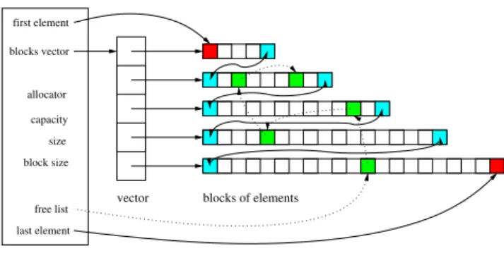
Figure 1 illustrates the memory layout of the Compact_container. In the example, 5 blocks are allocated and 5 elements are on the free list (in green). We see that the container maintains pointers to the first and last elements (in red) for the iterator’s needs, and for the same reason all blocks are chained, hence the first and last elements of each block (in blue) are not usable. It also maintains the size (the number of live elements, here 50), the capacity (the maximum achievable size without re-allocation, here 55) and the current block size (here 21). In addition, but not strictly necessary, a vector stores the pointers to all blocks, in order to be able to reach the blocks more efficiently when allowing block de-allocation. Indeed, de-allocating a block in the middle of the blocks sequence (which could be useful to release memory) prevents the predictability of the size of each block, and hence the constant time reachability of the end of the blocks, which is otherwise the only way to access the next block. A practical advantage of this is that it allows to destroy a container in
first element vector last element free list blocks vector block size size capacity allocator Compact container blocks of elements
Figure 1: Compact_container memory layout.
O(√n) time instead of O(n), when the element’s destructor is trivial (completely optimized
away) as is often the case.
This design is very efficient as the needs for the iterator cause no overhead for live elements, and addition and removal of elements are just a few simple operations in most cases. Memory locality is also rather good overall: if only additions are performed, then the elements become consecutive in memory, and the iterator order is even the order of the additions. For alternating sequences of additions and removals, like a container of cells of an incremental Delaunay triangulation might see, the locality is still relatively good if the points are inserted in a spatial local order such as Hilbert or BRIO. Indeed, for a point insertion, the Bowyer-Watson algorithm erases connected cells, which are placed consecutively on the free list, and requires new cells, consecutively as well, from the free list, to re-triangulate the hole. So, even if some shuffling is unavoidable, this simple mechanism takes care of maintaining a relatively good locality of the data on a large scale.
Experimental comparison We have measured the time and memory space used by the
computation of a (sequential) 3D Delaunay triangulation of 1 million random points using CGAL, only changing the containers used internally to store the vertices and cells. The experiment was conducted on a MacBook Pro with a 2.33 GHz 32 bit Intel processor, 2 GB of RAM, and using the GCC compiler version 4.3.2 with optimization level 2. Using list, the program took 19.3 seconds and used 389 MB of RAM, while using our Compact_container it took 13.3 seconds and used 288 MB. The optimal memory size would have been 258 MB, as computed by the number of vertices and cells times their respective memory sizes (28 and 36 bytes respectively). This means that the internal memory overhead was 51% for list and only 11% for Compact_container.
We also performed the same experiment, this time for 10 million points, on a 64 bit machine with 16 GB of RAM under Linux. We observed almost the same internal memory overheads but with a smaller time difference of still 28%. For 30 million points, the internal memory overhead for Compact_container went down to 8.6%.
Fragmentation Some applications like mesh simplification build a large triangulation and then select a significant fraction of the vertices and remove them. In such cases, the
Compact_containeris not at its best, since it never releases memory blocks to the system
automatically. In fact, such an application would produce a very large free list, with the free elements being spread all over the blocks, producing high fragmentation. Moreover, the iterator would be slower as it skips the free elements one by one (this would even violate the complexity requirements of standard iterators whose increment and decrement operations are required to be amortized constant time). The Compact_container does not provide a specific function to handle this issue, and the recommended way to improve the situation is to copy the container, which moves its elements to a new, compact area.
Parallelization Using the Compact_container in the parallel setting required some changes.
It should be possible to have a shared data structure (e.g. a triangulation class), and change it using several threads concurrently. So the container is required to support concurrent addition and removal operations. At such a low level, thread safety needs to be achieved in an efficient way, as taking locks for each operation would necessarily degrade performance, with lots of expected contention.
The way we extended the Compact_container class is that we chose to have one inde-pendent free list per thread, which completely removed the need for synchronization in the removal operation. Moreover, considering the addition operation, if the thread’s free list is not empty, then a new element can be taken from its head without need for synchronization either, and if the free list is empty, the thread allocates a new block, and adds its elements to its own free list. Therefore, the only synchronization needed is when allocating a new block, since (a) the allocator may not be thread-safe and (b) all blocks need to be known by the container class so a vector of block pointers is collected. Since the size of the blocks
is growing as O(√n), the relative overhead due to synchronization also decreases as the
structure grows.
Note that, since when allocating a new block, all its elements are put on the current thread’s free list, it means that they will initially be used only by this thread, which also helps locality in terms of threads. However, once an element has been added, another thread can remove it, putting it on his own free list. So in the end, there is no guarantee that elements in a block are “owned” forever by a single thread, some shuffling can happen. Nevertheless, we should obtain a somewhat “global locality” in terms of time, memory, and thread (and geometry thanks to spatial sorting, if the container is used in a geometric context).
A minor drawback of this approach is that free elements are more numerous, and the
wasted memory is expected to be O(t√n) for t threads, each typically wasting a part of a
block (assuming an essentially incremental algorithm, since here as well, no block is released back to the allocator).
Element addition and removal are operations which are then allowed to be concurrent. Read-only operations like iterating can also be performed concurrently.
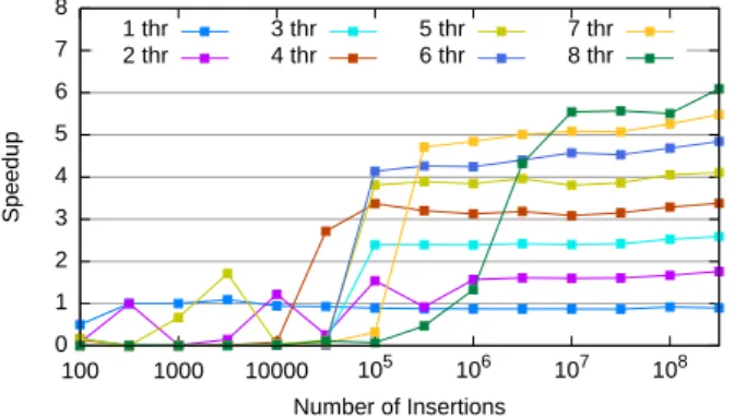
Benchmark Figure 2 shows a synthetic benchmark of the parallel Compact_container alone, by performing essentially parallel additions together with 20% of interleaved deletions, and comparing it to the sequential original version. We see that the container scales very nicely with the number of threads as soon as a minimum number of elements is reached. This benchmark is synthetic, since no computation is performed between the insertions and deletions. We can hope that using it for geometric algorithms will prove it useful even with lower numbers of elements, although this is hard to measure.
0 1 2 3 4 5 6 7 8 100 1000 10000 105 106 107 108 Speedup Number of Insertions 1 thr 2 thr 3 thr 4 thr 5 thr 6 thr 7 thr 8 thr
Figure 2: Speedups obtained for the compact container with additions and 20% of deletions.
4
Spatial sorting
Problem definition and algorithm Many geometric algorithms implemented in CGAL
are incremental, and their speed depends on the order of insertion for locality reasons in geometric space and in memory. For cases where some randomization is still required for complexity reasons, the Biased Randomized Insertion Order method [4] (BRIO) is an optimal compromise between randomization and locality. Given n randomly shuffled points and a parameter α, BRIO recurses on the first ⌊αn⌋ points, and spatially sorts the remaining points. For these reasons, CGAL provides algorithms to sort points along a Hilbert space-filling curve as well as a BRIO.
Since spatial sorting (either strict Hilbert or BRIO) is an important substep of several CGAL algorithms, the parallel scalability of those algorithms would be limited if the spatial sorting was computed sequentially, due to Amdahl’s law. For the same reason, the random shuffling should also be parallelized.
The sequential implementation uses a divide-and-conquer (D&C) algorithm. It recur-sively partitions the set of points with respect to a dimension, taking the median point as pivot. The dimension is then changed and the order is reversed appropriately for each recursive call, such that the process results in arranging the points along a Hilbert curve.
0 1 2 3 4 5 100 1000 10000 100000 106 107 Speedup Input Size 8 thr 7 thr 6 thr 5 thr 4 thr 3 thr 2 thr 1 thr
Figure 3: Speedup for 2D spatial sort.
0 1 2 3 4 5 100 1000 104 105 106 107 108 Speedup Input Size 8 thr 7 thr 6 thr 5 thr 4 thr 3 thr 2 thr 1 thr
Figure 4: Speedup for kd tree construction. Parallelizing this algorithm is straightforward. The partitioning is done by calling the parallel nth_element function, and the parallel random_shuffle for BRIO. The recursive subproblems are processed by newly spawned OpenMP tasks.
Experimental results The speedup (ratio of the running times between the parallel and
sequential versions) obtained for 2D Hilbert sorting are shown in Figure 3. For a small number of threads, the speedup is good for problem sizes greater than 1000 points, but the efficiency drops to about 60% for 8 threads. We blame the memory bandwidth limit for this decline. The results for the 3D case are very similar except that the speedup is 10–20% less
for large inputs. Note that, for reference, the sequential code sorts 106
random points in 0.39s.
5
Kd tree construction
Problem definition and algorithm A kd tree [5] is a fundamental spatial search data
structure, allowing efficient queries for the subset of points contained in an orthogonal query box.
In principle, a kd tree is a dynamic data structure. However, it is unclear how to do balancing dynamically, so worst-case running time bounds for the queries are only given for trees constructed offline. Also, insertion of a single point is hardly parallelizable. Thus, we describe here the construction of the kd tree for an initially given set of points.
The approach is actually quite similar to spatial sorting. The algorithm partitions the data and recursively constructs the subtrees for each half in parallel.
Experimental results The speedup for the parallel kd tree construction of 3-dimensional
random points with double-precision Cartesian coordinates is shown in Figure 4. The achieved speedup is similar to the spatial sort case, a little less for small inputs. Note
6
D-dimensional box intersection
Problem definition We consider the problem of finding all intersections among a set of
n iso-oriented d-dimensional boxes. This problem has applications in fields where complex geometric objects are approximated by their bounding box in order to filter them against some predicate.
Algorithm We parallelize the algorithm proposed by Zomorodian and Edelsbrunner [25],
which is already used for the sequential implementation in CGAL, and proven to perform well in practice. The algorithm is described in terms of nested segment and range trees,
leading to an O(n logd
n) space algorithm in the worst case. Since this is too much space overhead, the trees are not actually constructed, but traversed on the fly. So we end up with a D&C algorithm using only logarithmic extra memory (apart from the possibly quadratic output). For small subproblems below a certain cutoff size, a base-case quadratic-time algorithm is used to check for intersections.
Again, the D&C paradigm promises good parallelization opportunities. We can assign the different parts of the division to different threads, since their computation is usually independent.
However, we have a detail problem in the two most important recursive conquer calls: the data they process is in general not disjoint. Worse, although they do not change the input elements, the recursive calls may reorder them. This is a problem for parallelization, since we cannot just pass the same data to both calls if they are supposed to run in parallel.
Thus, we have to copy2
.
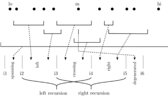
Let us describe this divide step in more detail. The problem is solved dimension by dimension, recursively. In each level, the input consists of two sequences: points and inter-vals. A pivot point m is determined in a randomized fashion, and the sequence of points is partitioned accordingly. The two parts are passed to the two recursive calls, accompanied by the respective intervals. For the left part, all intervals are chosen that have their left end
point left from m. For the right part, all intervals that have their right end point (strictly3)
right of m. Of course, these two sets of intervals can overlap, common elements are exactly the ones spanning m. See Figure 5 for an illustration.
We can reorder the original sequence such that the intervals to the left are at the be-ginning, the intervals to the right at the end, and the common intervals being placed in the middle. Intervals not contained in any part (degenerated to an empty interval in this dimension) can be moved behind the end. Now, we have five consecutive ranges in the
complete sequence. [i1, i2) are the intervals spanning the whole region. They are handled
separately. [i2, i3) and [i4, i5) are respectively the intervals for the left and right recursion
steps only. [i3, i4) are the intervals for both the left and the right recursion step. [i5, i6) are
the ignored degenerate intervals.
2
We could take pointers instead of full objects in all cases since they are only reordered. But this saves only a constant factor and leads to cache inefficiency due to lacking locality, see [1]
3
Whether the comparisons are strict or not, depends on whether the boxes are open or closed. This does not change anything in principle. Here, we describe only the open case.
m
lo hi
i1 i2 i3 i4 i5 i6
left recursion right recursion
spanning left right cros sing degenerated
Figure 5: Partitioning the sequence of inter-vals.
left continuous sequence right continuous sequence
input left rec
right rec
Cas
e 1
left continuous sequence right continuous sequence
input left rec
right rec
Cas
e 2
left continuous sequence right continuous sequence
input left rec
right rec
Cas
e 3
Figure 6: Treating the split sequence of
intervals. Fat lines denote copied
ele-ments.
To summarize, we need [i2, i4) for the left recursion step, and [i3, i5) for the right one,
which overlap. The easiest way to solve the problem is to either copy [i2, i4) or [i3, i5).
But this is inefficient, since for well-shaped data sets (having a relatively small number of
intersections), the part [i3, i4), which is the only one we really need to duplicate, will be quite
small. Thus, we will in fact copy only [i3, i4) to a newly allocated sequence [i′3, i′4). Now
we can pass [i2, i4) to the left recursion, and the concatenation of [i′3, i′4) and [i4, i5) to the
right recursion. However, the concatenation must be made implicitly only, to avoid further copying. The danger arises that the number of these gaps might increase in a sequence range as recursion goes on, leading to overhead in time and space for traversing them, which counteracts the parallel speedup.
However, we will now prove that this can always be avoided. Let a continuous sequence be the original input or a copy of an arbitrary range. Let a continuous range be a range of a continuous sequence. Then, a sequence range consisting of at most two continuous ranges always suffices for passing a partition to a recursive call.
Proof: We can ignore the ranges [i1, i2) and [i5, i6), since they do not take part in this
overlapping recursion, so it is all about [i2, i3), [i3, i4), and [i4, i5). Induction begin: The
original input consists of one continuous range. Induction hypothesis: [i1, i6) consists of at
most two continuous ranges. Inductive step: [i1, i6) is split into parts. If i3is in its left range,
we pass the concatenation of [i2, i3)[i′3, i′4) (two continuous ranges) to the left recursion step,
and [i3, i5) to the right one. Since the latter is just a subpart of [i1, i6), there cannot be
additional ranges involved. If i3 is in the right range of [i1, i6), we pass the concatenation
of [i′
3, i′4)[i4, i5) (two continuous ranges) to the right recursion step, and [i2, i4) to the right
one. Since the latter is just a subpart of [i1, i6), there cannot be additional ranges involved.
The three cases and their treatment are shown in Figure 6.
Deciding whether to subtask The general question is how many tasks to create,
load balancing. On the other hand, the number of tasks T should be kept low in order to limit the memory overhead. In the worst case, all data must be copied for the recursive call, so the size of additional memory can grow with O(T · n). Generally speaking, only concurrent tasks introduce disadvantages, since the additional memory is deallocated after having been used. So if we can limit the number of concurrent tasks to something lower than T , that number will count. There are several criteria that should be taken into account when deciding whether to spawn a task.
• Spawn a new task if the problem to process is large enough (both the number of
intervals and the number of points are beyond a certain threshold value cmin (tuning
parameter)). This strategy strives to amortize for the task creation and scheduling overhead. However, in this setting, the running time overhead can be proportional to the problem size, because of the copying. In the worst case, a constant share of the data must be copied a logarithmic number of times, leading to excessive memory usage.
• Spawn a new task if there are less than a certain number of tasks tmax (tuning
pa-rameter) in the task queue. Since OpenMP does not allow to inspect its internal task queue, we have to count the number of currently active tasks manually, using atomic operations on a counter. This strategy can effectively limit the number of concurrently processed tasks, and so the memory consumption indirectly.
• Spawn a new task if there is memory left from a pool of size s (tuning parameter). This strategy can effectively limit the amount of additional memory, guaranteeing correct termination.
In fact, we combine the three criteria to form a hybrid. All three conditions must be fulfilled.
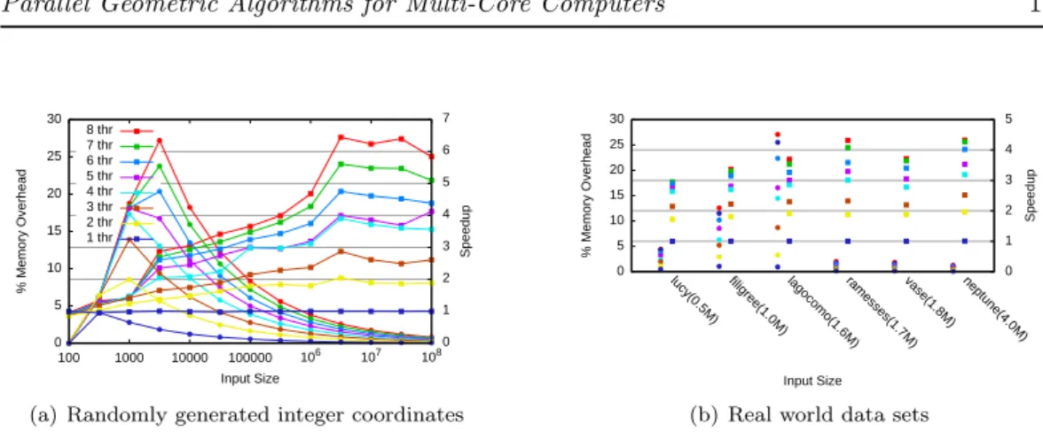
Experimental results 3-dimensional boxes with integer coordinates were randomly
gen-erated as in [25] such that the expected number of intersections for n boxes is n/2.
For the results in Figure 7(a), we used cmin = 100, tmax= 2 · t, and s = 1 · n, where t
is the number of threads. The memory overhead is limited to 100%, but as we can see, the
relative memory overhead is much lower in practice, below 20% for not-too-small inputs4
. The speedups are quite good, reaching more than 6 for 8 cores, and being just below 4 for
4 threads. Note that, for reference, the sequential code performs the intersection of 106
boxes in 1.86s.
Figure 7(b) shows the results for real-world data. We test 3-dimensional models for self-intersection, by approximating each triangle with its bounding box, which is a common application. The memory overhead stays reasonable. The speedups are a bit worse than for the random input of the equivalent size. This could be due to the much higher number of found intersections (∼ 7n).
4
The memory overhead numbers refer to the algorithmic overhead only. For software engineering reasons, e. g. preserving the input sequence, the algorithm may decide to copy the whole input in a preprocessing step.
0 5 10 15 20 25 30 100 1000 10000 100000 106 107 108 0 1 2 3 4 5 6 7 % Memory Overhead Speedup Input Size 8 thr 7 thr 6 thr 5 thr 4 thr 3 thr 2 thr 1 thr
(a) Randomly generated integer coordinates
0 5 10 15 20 25 30
lucy(0.5M) filigree(1.0M) lagocomo(1.6M)ramesses(1.7M)vase(1.8M) neptune(4.0M) 0
1 2 3 4 5 % Memory Overhead Speedup Input Size (b) Real world data sets
Figure 7: Intersecting boxes. Speedup is denoted by squares, relative memory overhead by circles.
7
Bulk insertion into 3D Delaunay triangulations
Given a set S of n points in Rd, a triangulation of S partitions the convex hull of its points
into simplices (cells) with vertices in S. The Delaunay triangulation DT (S) is characterized by the empty sphere property that states the circumsphere of any cell does not contain any other point of S in its interior. A point q is said to be in conflict with a cell in DT (S), if it belongs to the interior of the circumsphere of that cell, and the conflict region of q is defined as the set of all such cells. The conflict region is non-empty, since it must contain at least the cell the point lies in, and is known to be connected.
Related work Perhaps the most direct method for a parallel scheme is to use the D&C
paradigm, recursively partitioning the point set into two subregions, computing solutions for each subproblem, and finally merging the partial solutions to obtain the triangulation. Either the divide or the merge step are usually quite complex, though. Moreover, bulk insertions of points in already computed triangulations is not supported well, as required for many mesh refinement algorithms.
A feasible parallel 3D implementation was first presented by Cignoni et al. [12]. In a complex divide step, the Delaunay wall is constructed, the set of cells splitting regions, before working in parallel in isolation. As pointed out by the authors, this method suffers from limited scalability due to the cost of wall construction. It achieves only a 3 times speedup triangulating 8000 points on an 8-processor nCUBE 2 hypercube. Cignoni et al. [11] also designed an algorithm where each processor triangulates its set of points in an incremental fashion. Although this method does not require a wall, tetrahedra with vertices belonging to different processors are constructed multiple times. A speedup of 5.34 was measured for 8 processors for 20000 uniformly distributed points.
Lee et al. [18], focusing on distributed memory systems, improved this algorithm by exploiting a projection-based partitioning scheme [7], eliminating the merging phase. They
showed that a simpler non-recursive version of this procedure lead to better results for almost all considered inputs. The algorithm was implemented on an INMOS TRAM network of 32 T800 processors and achieved a 6.5 times speedup on 8 processors with 10000 randomly distributed points. However, even their best partitioning method took 75% of the total elapsed time.
The method of Blelloch et al. [7] treats the 2D case using the well-known relation with 3D convex hulls. Instead of directly solving a convex hull problem, another reduction step to 2D lower hull is carried out. It was shown that the resulting hull edges are already Delaunay edges, but the algorithm requires an additional step to construct missing edges. They obtained a speedup of 5.7 on 8 CPUs with uniform point distribution on a shared-memory SGI Power Challenge.
More recently, parallel algorithms avoiding the complexity of the D&C algorithms were published. Kohout et al. [17] proposed parallelizing randomized incremental construction. This is based on the observation that topological changes caused by point insertion are likely to be extremely local. When a thread modifies the triangulation, it acquires exclusive access to the containing tetrahedron and a few cells around it. For a three-dimensional uniform distribution of half a million points, their algorithm reaches speedups of 1.3 and 3.6 using 2 and 4 threads, respectively on a 4 processors Intel Itanium at 800MHz with a 4MB cache and 4GB RAM. We observed, however, that their sequential speed is about one order of magnitude lower than the CGAL implementation, which would make any parallel speedup comparison unfair.
Another algorithm based on randomized incremental construction was proposed by Bland-ford et al. [6]. It employs a compact data structure and follows a Bowyer-Watson ap-proach [9, 24], maintaining an association between uninserted points and their containing tetrahedra [13]. A coarse triangulation is sequentially built using a separate triangulator (Shewchuk’s Pyramid [21]) before threads draw their work from the subsets of points asso-ciated with these initial tetrahedra. This is done in order to build an initial triangulation sufficiently large so as to avoid thread contention. For uniformly distributed points, their algorithm achieved a relative speedup of 46.28 on 64 1.15-GHz EV67 processors with 4GB RAM per processor, spending 6% to 8% of the total running time in Pyramid, but with the smallest instance consisting of 23 million points. Their work targeted huge triangulations
(230.5 points on 64 processors), as they also use compression schemes which would only slow
things down for more common input sizes. In this paper, we are also interested in speeding up smaller triangulations, whose size ranges from a thousand to millions of points (in fact, we tested up to 31 million points, which fits in 16GB of memory).
Sequential framework CGAL provides 2D and 3D incremental algorithms [8] and a
similar approach has also been implemented in d dimensions [16]. After a spatial sort using a BRIO, points are iteratively inserted using a locate step followed by an update step. The locate step finds the cell containing q using a remembering stochastic walk [14] that starts at some cell incident to the vertex created by the previous insertion, and navigates using orientation tests and the adjacency relations between cells. The update step determines the
conflict region of q using the Bowyer-Watson algorithm [9, 24], that is, by checking the empty sphere property for all the neighbors of the cell containing q, recursing using the adjacency relations again. The conflict region is then removed, creating a “hole”, and the triangulation is updated by creating new cells connecting q to the vertices on the boundary of the “hole”. From a storage point of view, a vertex stores its point and a pointer to an incident cell, and a cell stores pointers to its vertices and neighbors. Vertices and cells are themselves stored in two compact containers (see Section 3). Note that there is also an infinite vertex linked to the convex hull through infinite cells. Also worth noting for the sequel is that once a vertex in created, it never moves (this paper does not consider removing vertices), therefore its address is stable, while a cell can be destroyed by subsequent insertions.
Parallel algorithm We attack the problem of constructing DT (S) in parallel by allowing
concurrent insertions into the same triangulation, and spreading the input points over all threads. Our scheme is similar to [6, 17], but with different point location, load management mechanisms and locking strategies.
First, a bootstrap phase inserts a small randomly chosen subset S0 of the points using
the sequential algorithm, in order to avoid contention for small data sets. The size of S0
is a tuning parameter. Next, the remaining points are Hilbert-sorted in parallel, and the resulting range is divided into almost equal parts attributed to all threads. Threads then insert their points using an algorithm similar to the sequential case (location and updating steps), but with the addition that threads protect against concurrent modifications to the same region of the triangulation. This protection is performed using fine-grained locks stored in the vertices. Concerning the storage, the thread-safe compact container described in Section 3 has been used.
Locking and retreating Threads read the data structure during the locate step, but
only the update step locally modifies the triangulation. To guarantee threads safety, both procedures lock and unlock some vertices.
A lock conflict occurs when a thread attempts to acquire a lock already owned by another thread. Systematically waiting for the lock to be released is not an option since a thread may already own other locks, potentially leading to a deadlock. Therefore, lock conflicts are handled by priority locks where each thread is given a unique priority (totally ordered). If the acquiring thread has a higher priority it simply waits for the lock to be released. Otherwise, it retreats, releasing all its locks and restarting an insertion operation, possibly with a different point. This approach avoids deadlocks and guarantees progress. Note that the implementation of priority locks needs attention, since comparing the priority and
acquiring a lock need to be performed atomically5
.
Interleaving A retreating thread should continue by inserting a far away point,
hope-fully leaving the area where the higher priority thread is operating. On the other hand,
5
Since this is not efficiently implementable using OpenMP primitives, we used our own implementation using spin locks based on hardware-supported atomic operations.
inserting a completely unrelated point is impeded by the lack of a expectedly close starting point for the locate step. Therefore, each thread divides its own range into several parts of roughly equal sizes, and keeps a reference vertex for each of them to restart point location. The number of these parts is a tuning parameter of the algorithm. It starts to insert points from the first part. Each time it has to retreat, it switches to the next part in a round-robin fashion. Because the parts are constructed from disjoint ranges of the Hilbert-sorted sequence, vertices taken from different parts are not particularly likely to be spatially close and trigger conflicts. This results in an effective compromise between locality of reference and conflict avoidance.
Locking strategies There are several ways of choosing the vertices to lock.
A simple strategy consists in locking the vertices of all cells a thread is currently consid-ering. During the locate step, this means locking the d + 1 vertices of the current cell, then, when moving to a neighboring cell, locking the opposite vertex and releasing the unneeded lock. During the update step, all vertices of all cells in conflict are locked, as well as the vertices of the cells which share a face with those in conflict, since those cells are also tested for the insphere predicate, and at least one of their neighbor pointers will be updated. Once the new cells are created and linked, the acquired locks can be released. This strategy is simple and easily proved correct. However, as the experimental results show, high degree vertices become a bottleneck with this strategy.
We therefore propose an improved strategy that reduces the number of locks and partic-ularly avoids locking high degree vertices as much as possible. It works as follows: reading a cell requires locking at least two of its vertices, changing a cell requires locking at least d of its vertices, and changing the incident cell pointer of a vertex requires it to be locked. This rule implies that a thread can change a cell without others reading it, but it allows some concurrency among reading operations. Most importantly, it allows reading and changing cells without locking all their vertices, therefore giving some leeway to avoid locking high degree vertices. During the locate step, keeping at most two vertices locked is enough: when using neighboring relations, choosing a vertex common with the next cell is done by choos-ing the one closest to q (thereby discardchoos-ing the infinite vertex). Durchoos-ing the update step, a similar procedure needs to be followed except that once a cell is in conflict, it needs to have d vertices locked, which allows to exclude the furthest vertex from q, with the following caveat: all vertices whose incident cell pointer point to this cell also need to be locked. This measure is necessary so that other threads starting a locate step at this vertex can access the incident cell pointer safely. Once the new cells are created and linked, the incident cell pointers of the locked vertices are updated (and those only) and the locks are released.
The choice of attempting to exclude the furthest vertex is motivated by the consideration of needle shaped simplices for which it is preferable to avoid locking the singled-out vertex as it has a higher chance of being of high degree. For example, the infinite vertex will be locked only when a thread needs to modify the incident cell it points to. Similarly, performing the locate step in a surfacic data set will likely lock vertices which are on the same sheet as q.
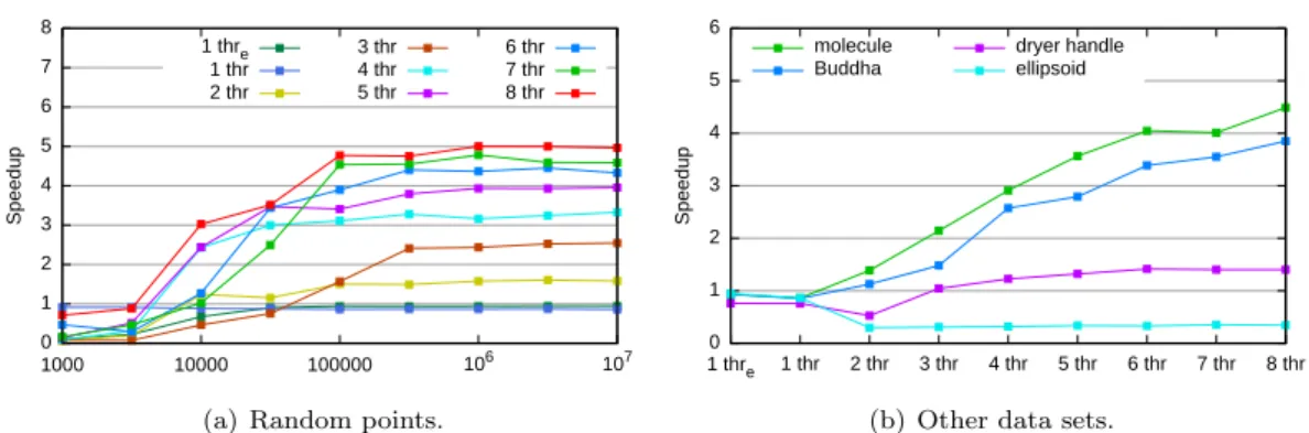
0 1 2 3 4 5 6 7 8 1000 10000 100000 106 107 Speedup 1 thre 1 thr 2 thr 3 thr 4 thr 5 thr 6 thr 7 thr 8 thr
(a) Random points.
0 1 2 3 4 5 6 1 thre 1 thr 2 thr 3 thr 4 thr 5 thr 6 thr 7 thr 8 thr Speedup molecule Buddha dryer handle ellipsoid
(b) Other data sets.
Figure 8: Speedups for 3D Delaunay triangulation.
Experimental results We have implemented our parallel algorithm in 3D using the
sim-ple locking strategy.6
We carried out experiments in 3D on five different point sets, including two synthetic and three real-world data. The synthetic data consist of evenly distributed points in a cube, and 1 million points lying on the surface of an ellipsoid of axes lengths 1, 2 and 3. The real instances are composed of points on the surfaces of a molecule, a Buddha statue, and a dryer handle containing 525K, 543K and 50K points respectively. For
reference, the original sequential code computes a triangulation of 106
random points in 16.57s.
Running time measurement has proven very noisy in practice, especially for small in-stances. For this reason, we iterated the measurements a number of times depending on the input size.
Figures 8(a) and 8(b) show the achieved speedups. We observe that a speedup of almost
5 is reached with 8 cores for 105random points or more. However, we note that the surfacic
data sets are not so positively affected, and we blame the simple locking strategy for that.
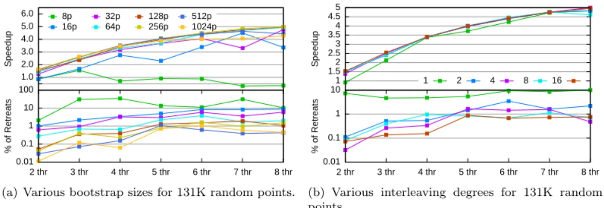
Tuning parameters In order to empirically select generally good values for the
pa-rameters which determine the size of S0 (we chose 100p, where p is the number of threads)
and the interleaving degree (we chose 2), we have studied their effect on the speedup as well as the number of retreats. Figures 9(a) and 9(b) show the outcome of these tests for the random data set, while Appendix A provides figures for other input. A small value like 2 for the interleaving degree already provides most of the benefit of the technique. The bootstrap size has no significant influence on the running time for large data sets, but it affects the number of retreats which may affect small data sets.
6
We lacked time to properly implement and benchmark the improved locking strategy, but we plan to show its results instead in the final version of paper, if the improvement is here as planned.
1.0 2.0 3.0 4.0 5.0 6.0 Speedup 8p 16p 32p 64p 128p 256p 512p 1024p 0.01 0.1 1 10 100 2 thr 3 thr 4 thr 5 thr 6 thr 7 thr 8 thr % of Retreats
(a) Various bootstrap sizes for 131K random points.
1 1.5 2 2.5 3 3.5 4 4.5 5 Speedup 1 2 4 8 16 0.01 0.1 1 10 2 thr 3 thr 4 thr 5 thr 6 thr 7 thr 8 thr % of Retreats
(b) Various interleaving degrees for 131K random points.
Figure 9: Evaluating tuning parameters for 3D Delaunay triangulation.
8
Conclusion and future work
We have described new parallel algorithms for four fundamental geometric problems, espe-cially targeted at shared-memory multi-core architectures, which are increasingly available. These are d-dimensional spatial sorting of points, kd-tree construction, axis-aligned box intersection computation, and bulk insertion of points in Delaunay triangulations. Exper-iments in 3D show significant speedup over their already efficient sequential original coun-terparts, as well as good comparison to previous work for the Delaunay computation for problems of reasonnable size.
In the future, we plan to extend our implementation to cover more algorithms, and then submit it for integration in CGAL once it is stable enough, to serve as a first stone towards a parallel mode which CGAL users will be able to benefit from transparently.
Acknowledgments This work has been supported by the INRIA Associated Team GENEPI,
the NSF-INRIA program REUSSI, the Brazilian CNPq sandwich PhD program, and the French ANR program TRIANGLES. We also thank Manuel Holtgrewe his work on the parallel kd-trees.
References
[1] The CGAL manual on the box intersection performance. http://www.cgal.org/ Manual/3.3/doc_html/cgal_manual/Box_intersection_d/Chapter_main.html# Section_47.8.
[2] Alok Aggarwal, Bernard Chazelle, Leonidas J. Guibas, Colm Ó’Dúnlaing, and Chee-Keng Yap. Parallel computational geometry. Algorithmica, 3(1–4):293–327, 1988. [3] Selim G. Akl and Kelly A. Lyons. Parallel computational geometry. Prentice-Hall, Inc.,
Upper Saddle River, NJ, USA, 1993.
[4] Nina Amenta, Sunghee Choi, and Günter Rote. Incremental constructions con brio. In SCG ’03: Proceedings of the nineteenth annual symposium on Computational geometry, pages 211–219, 2003.
[5] Jon Louis Bentley. Multidimensional binary search trees used for associative searching. Commun. ACM, 18(9):509–517, 1975.
[6] Daniel K. Blandford, Guy E. Blelloch, and Clemens Kadow. Engineering a compact parallel Delaunay algorithm in 3D. In SCG ’06: Proceedings of the twenty-second annual symposium on Computational geometry, pages 292–300, 2006.
[7] Guy E. Blelloch, J. C. Hardwick, G. L. Miller, and D. Talmor. Design and implemen-tation of a practical parallel Delaunay algorithm. Algorithmica, 24(3):243–269, 1999. [8] Jean-Daniel Boissonnat, Olivier Devillers, Sylvain Pion, Monique Teillaud, and Mariette
Yvinec. Triangulations in CGAL. Comput. Geom. Theory Appl., 22:5–19, 2002. [9] A. Bowyer. Computing Dirichlet tesselations. The Computer Journal, 24(2):162–166,
1981.
[10] Anita Liu Chow. Parallel algorithms for geometric problems. PhD thesis, University of Illinois, Urbana-Champaign, IL, USA, 1980.
[11] P. Cignoni, D. Laforenza, C. Montani, R. Perego, and R. Scopigno. Evaluation of
parallelization strategies for an incremental Delaunay triangulator in E3. Concurrency:
Practice and Experience, 7(1):61–80, 1995.
[12] P. Cignoni, C. Montani, R. Perego, and R. Scopigno. Parallel 3D Delaunay triangula-tion. Computer Graphics Forum, 12(3):129–142, 1993.
[13] Kenneth L. Clarkson and Peter W. Shor. Applications of random sampling in compu-tational geometry, ii. Discrete Comput. Geom., 4(5):387–421, 1989.
[14] Olivier Devillers, Sylvain Pion, and Monique Teillaud. Walking in a triangulation. International Journal of Foundations of Computer Science, 13(2):181–199, 2002.
[15] Michael Hoffmann, Lutz Kettner, Sylvain Pion, and Ron Wein. STL extensions for CGAL. In CGAL Editorial Board, editor, CGAL User and Reference Manual. 3.3 edition, 2007.
[16] Samuel Hornus and Jean-Daniel Boissonnat. An efficient implementation of Delaunay triangulations in medium dimensions. Research Report 6743, INRIA, 2008. http: //hal.inria.fr/inria-00343188.
[17] Josef Kohout, Ivana Kolingerová, and Jiří Žára. Parallel Delaunay triangulation in E2
and E3
for computers with shared memory. Parallel Computing, 31(5):491–522, 2005. [18] Sangyoon Lee, Chan-Ik Park, and Chan-Mo Park. An improved parallel algorithm for
Delaunay triangulation on distributed memory parallel computers. Parallel Processing Letters, 11(2/3):341–352, 2001.
[19] Yuanxin Liu and Jack Snoeyink. A comparison of five implementations of 3D delaunay tessellation. In Jacob E. Goodman, János Pach, and Emo Welzl, editors, Combina-torial and Computational Geometry, volume 52 of MSRI Publications, pages 439–458. Cambridge University Press, 2005.
[20] James Reinders. Intel Threading Building Blocks: Outfitting C++ for Multi-core Pro-cessor Parallelism. O’Reilly Media, Inc., 2007.
[21] Jonathan R. Shewchuk. Tetrahedral mesh generation by Delaunay refinement. In Proc. 14th Annu. ACM Sympos. Comput. Geom., pages 86–95, 1998.
[22] Johannes Singler and Benjamin Kosnik. The libstdc++ parallel mode: Software engi-neering considerations. In International Workshop on Multicore Software Engiengi-neering (IWMSE), 2008.
[23] Johannes Singler, Peter Sanders, and Felix Putze. MCSTL: The multi-core standard template library. In Euro-Par ’07: Proceedings of the thirteenth European Conference on Parallel and Distributed Computing, pages 682–694, 2007.
[24] D. F. Watson. Computing the n-dimensional Delaunay tesselation with application to Voronoi polytopes. The Computer Journal, 24(2):167–172, 1981.
[25] Afra Zomorodian and Herbert Edelsbrunner. Fast software for box intersections. Int. J. Comput. Geometry Appl., 12(1-2):143–172, 2002.
Appendix
A
Tuning the parallel Delaunay algorithm
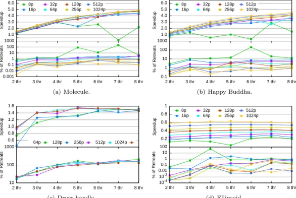
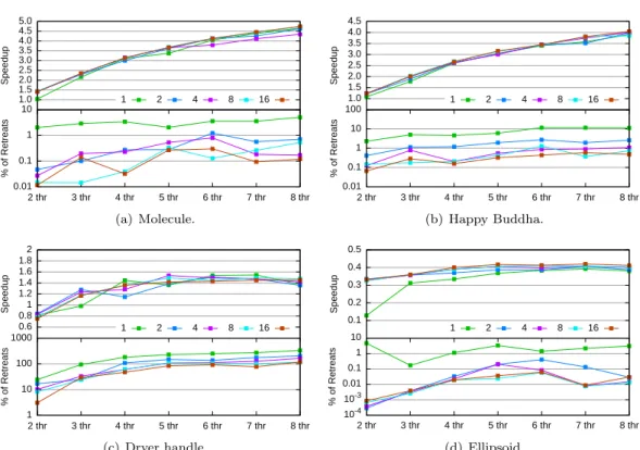
We have shown that our algorithm scales well on random distributions and some surfacic data sets. We introduced the bootstrap size and interleaving degree as tuning parameters which are important in controlling the number of retreats, and we have presented their effect for 131K random points. In this section, we provide several other figures showing detailed measurements on the effect of the tuning parameters for the Delaunay algorithm on various inputs. In addition, we show the breakdown of the running time of our algorithm over different instances.
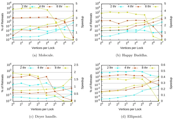
We tried out different bootstrap sizes (see Figure 10), as well as different interleaving degrees (see Figure 11). For the bootstrap, note that a value of 100p already gives enough locality for up to 8 threads to work. It can be noted that even a single increment in the interleaving degree was sufficient to obtain a significant reduction on the number of retreats. We also experimented with several (close-by) vertices sharing a lock, trying to save time on acquisitions and releases. However, the necessary indirection and the additional lock conflicts counteracted all improvement. Figure 12 illustrates the performance degradation introduced by using this mechanism (even with only one vertex per lock using the generic code). Figure 13 shows the effect of increasing the number of vertices per lock.
The cost of the algorithm can be broken down into several parts. These include the locate and update steps, as well as the bootstrap and spatial sort. Updating the triangu-lation requires, in turn, the determination of conflicting cells and the construction of new tetrahedra. There is also a minor part of time spent in copying points to a local array, and shuffling them randomly. All these tasks are performed in parallel. Figure 14 shows this breakdown for building the triangulation of 10M random points. It illustrates that point location and the Bowyer-Watson algorithm (shown as find conflict and create cells) are the main time consuming steps. The algorithm has approximately mantained the same behavior for random points, Buddha and molecule surfaces, achieving good scalability. It slows down, however, in the dryer handle and ellipsoid cases. This reveals the major defi-ciency of the current implementation, that of the infinite vertex which is connected to all points on the convex hull. So, in the ellipsoid case, the insertion of any point requires locking the infinite vertex. The dryer handle also shares this property, but in a minor scale. This can be observed in Figures 14(d) and 14(e).
1.0 2.0 3.0 4.0 5.0 6.0 Speedup 8p 16p 32p 64p 128p 256p 512p 1024p 0.001 0.01 0.1 1 10 100 1000 2 thr 3 thr 4 thr 5 thr 6 thr 7 thr 8 thr % of Retreats (a) Molecule. 1.0 2.0 3.0 4.0 5.0 6.0 Speedup 8p 16p 32p 64p 128p 256p 512p 1024p 0.1 1 10 100 1000 2 thr 3 thr 4 thr 5 thr 6 thr 7 thr 8 thr % of Retreats (b) Happy Buddha. 0.6 0.8 1.0 1.2 1.4 1.6 Speedup 64p 128p 256p 512p 1024p 10 100 1000 2 thr 3 thr 4 thr 5 thr 6 thr 7 thr 8 thr % of Retreats (c) Dryer handle. 0.2 0.4 0.6 0.8 1 Speedup 8p 16p 32p 64p 128p 256p 512p 1024p 10-4 10-3 0.01 0.1 1 10 100 2 thr 3 thr 4 thr 5 thr 6 thr 7 thr 8 thr % of Retreats (d) Ellipsoid.
Figure 10: Algorithm performance on different data sets with bootstrap sizes ranging from 8p to 1024p . Because of huge contention, dryer handle tests were carried out with bootstrap size starting at 64p.
1.0 1.5 2.0 2.5 3.0 3.5 4.0 4.5 5.0 Speedup 1 2 4 8 16 0.01 0.1 1 10 2 thr 3 thr 4 thr 5 thr 6 thr 7 thr 8 thr % of Retreats (a) Molecule. 1.0 1.5 2.0 2.5 3.0 3.5 4.0 4.5 Speedup 1 2 4 8 16 0.01 0.1 1 10 100 2 thr 3 thr 4 thr 5 thr 6 thr 7 thr 8 thr % of Retreats (b) Happy Buddha. 0.6 0.8 1 1.2 1.4 1.6 1.8 2 Speedup 1 2 4 8 16 1 10 100 1000 2 thr 3 thr 4 thr 5 thr 6 thr 7 thr 8 thr % of Retreats (c) Dryer handle. 0.1 0.2 0.3 0.4 0.5 Speedup 1 2 4 8 16 10-4 10-3 0.01 0.1 1 10 2 thr 3 thr 4 thr 5 thr 6 thr 7 thr 8 thr % of Retreats (d) Ellipsoid.
Figure 11: Performance of our algorithm with interleaving degrees 1, 2, 4, 8, and 16.
0 0.2 0.4 0.6 0.8 1 1.2 1 2 3 4 5 6 7 8 0.5 1 1.5 2 2.5 3 3.5 4 4.5 5 5.5 % of Retreats Speedup Number of Threads
not shared shared
Figure 12: Speedups and percentage of retreats during the construction of the 3D Delaunay
triangulation of 106
random points using individual and shared (1 vertex per lock) locking strategies. In both configurations, we have adopted bootstrap and interleaving degree equal to 100p and 2, respectively.
10-4 10-3 10-2 10-1 100 101 102 103 104 20 21 22 23 24 25 26 27 0 1 2 3 4 5 % of Retreats Speedup
Vertices per Lock 2 thr 4 thr 8 thr (a) Molecule. 10-4 10-3 10-2 10-1 100 101 102 103 104 20 21 22 23 24 25 26 27 0 1 2 3 4 5 % of Retreats Speedup
Vertices per Lock 2 thr 4 thr 8 thr (b) Happy Buddha. 10-2 10-1 100 101 102 103 104 20 21 22 23 24 25 26 27 0 0.5 1 1.5 2 2.5 % of Retreats Speedup
Vertices per Lock 2 thr 4 thr 8 thr (c) Dryer handle. 10-5 10-4 10-3 10-2 10-1 100 101 102 103 104 20 21 22 23 24 25 26 27 0 0.1 0.2 0.3 0.4 0.5 0.6 % of Retreats Speedup
Vertices per Lock 2 thr 4 thr 8 thr
(d) Ellipsoid.
0 50 100 150 200 250 seq 1 thre1 thr 2 thr 3 thr 4 thr 5 thr 6 thr 7 thr 8 thr Time (seconds) locate find conflict create cells bootstrap spatial sort random shuffle copy others
(a) Random distribution of 107 points. 0 2 4 6 8 10 12 14 seq 1 thre1 thr 2 thr 3 thr 4 thr 5 thr 6 thr 7 thr 8 thr Time (seconds) locate find conflict create cells bootstrap spatial sort random shuffle copy others (b) Molecule. 0 2 4 6 8 10 12 14 seq 1 thre1 thr 2 thr 3 thr 4 thr 5 thr 6 thr 7 thr 8 thr Time (seconds) locate find conflict create cells bootstrap spatial sort random shuffle copy others (c) Happy Buddha. 0 1 2 3 4 5 6 seq 1 thre1 thr 2 thr 3 thr 4 thr 5 thr 6 thr 7 thr 8 thr Time (seconds) locate find conflict create cells bootstrap spatial sort random shuffle copy others (d) Dryer handle. 0 10 20 30 40 50 60 seq 1 thre1 thr 2 thr 3 thr 4 thr 5 thr 6 thr 7 thr 8 thr Time (seconds) locate find conflict create cells bootstrap spatial sort random shuffle copy others (e) Ellipsoid.
Figure 14: Detailed profiling of the time spent in the various phases of the 3D Delaunay algorithm with bootstrap size 100p and interleaving degree 2.
Unité de recherche INRIA Futurs : Parc Club Orsay Université - ZAC des Vignes 4, rue Jacques Monod - 91893 ORSAY Cedex (France)
Unité de recherche INRIA Lorraine : LORIA, Technopôle de Nancy-Brabois - Campus scientifique 615, rue du Jardin Botanique - BP 101 - 54602 Villers-lès-Nancy Cedex (France)
Unité de recherche INRIA Rennes : IRISA, Campus universitaire de Beaulieu - 35042 Rennes Cedex (France) Unité de recherche INRIA Rhône-Alpes : 655, avenue de l’Europe - 38334 Montbonnot Saint-Ismier (France) Unité de recherche INRIA Rocquencourt : Domaine de Voluceau - Rocquencourt - BP 105 - 78153 Le Chesnay Cedex (France)