HAL Id: hal-00729008
https://hal.inria.fr/hal-00729008
Submitted on 7 Sep 2012
HAL is a multi-disciplinary open access
archive for the deposit and dissemination of
sci-entific research documents, whether they are
pub-lished or not. The documents may come from
teaching and research institutions in France or
abroad, or from public or private research centers.
L’archive ouverte pluridisciplinaire HAL, est
destinée au dépôt et à la diffusion de documents
scientifiques de niveau recherche, publiés ou non,
émanant des établissements d’enseignement et de
recherche français ou étrangers, des laboratoires
publics ou privés.
Fully Dynamic Maintenance of Arc-Flags in Road
Networks
Gianlorenzo d’Angelo, Mattia d’Emidio, Daniele Frigioni, Camillo Vitale
To cite this version:
Gianlorenzo d’Angelo, Mattia d’Emidio, Daniele Frigioni, Camillo Vitale. Fully Dynamic
Mainte-nance of Arc-Flags in Road Networks. 11th International Symposium on Experimental Algorithms
(SEA2012), Jun 2012, Bordeaux, France. pp.135-147, �10.1007/978-3-642-30850-5_13�. �hal-00729008�
Fully Dynamic Maintenance of Arc-Flags in
Road Networks
Gianlorenzo D’Angelo1, Mattia D’Emidio2, Daniele Frigioni2, and Camillo
Vitale2
1 MASCOTTE Project, I3S(CNRS/UNSA)/INRIA, France
gianlorenzo.d [email protected]
2 Dept. of Electrical and Information Engineering, University of L’Aquila, Italy
{mattia.demidio;daniele.frigioni}@univaq.it, [email protected]
Abstract. The problem of finding best routes in road networks can be solved by applying Dijkstra’s shortest paths algorithm. Unfortunately, road networks deriving from real-world applications are huge yielding unsustainable times to compute shortest paths. For this reason, great research efforts have been done to accelerate Dijkstra’s algorithm on road networks. These efforts have led to the development of a number of speed-up techniques, as for example Arc-Flags, whose aim is to com-pute additional data in a preprocessing phase in order to accelerate the shortest paths queries in an on-line phase. The main drawback of most of these techniques is that they do not work well in dynamic scenarios. In this paper we propose a new algorithm to update the Arc-Flags of a graph subject to edge weight decrease operations. To check the practical performances of the new algorithm we experimentally analyze it, along with a previously known algorithm for edge weight increase operations, on real-world road networks subject to fully dynamic sequences of op-erations. Our experiments show a significant speed-up in the updating phase of the Arc-Flags, at the cost of a small space and time overhead in the preprocessing phase.
1
Introduction
The problem of finding best connections in transportation networks has received a lot of attention in the last years. If travel times are assigned to the edges of the graph representing the network, this problem can be easily solved by applying Dijkstra’s algorithm to find the shortest path between two points. Unfortunately, transportation networks deriving from real-world applications tend to be huge yielding unsustainable times to compute shortest paths. For this reason, great research efforts have been done over the last decade to accelerate Dijkstra’s al-gorithm on typical instances of transportation networks, such as road or railway networks (see [5] for a recent overview). These research efforts have led to the development of a number of speed-up techniques, whose aim is to compute ad-ditional data in a preprocessing phase in order to accelerate the shortest paths queries during an on-line phase. However, most of the speed-up techniques devel-oped in the literature do not work well in dynamic scenarios, when edge weights
changes occur to the network due to traffic jams or delays of trains. In other words, the correctness of these speed-up techniques relies on the fact that the network does not change between two queries. Unfortunately, such situations arise frequently in practice. In order to keep the shortest paths queries correct, the preprocessed data need to be updated. The easiest way is to recompute the preprocessed data from scratch after each change to the network. This is in gen-eral unfeasible since even the fastest methods need too much time. In gengen-eral, the typical update operations that can occur on a network can be modelled as insertions and deletions of edges and edge weight changes (weight decrease and weight increase). When arbitrary sequences of the above operations are allowed, we refer to the fully dynamic problem, otherwise we refer to the partially dynamic problem; if only insertions and weight decrease (deletion and weight increase, re-spectively) operations are allowed, then the partially dynamic problem is known as the incremental (decremental, respectively) problem.
Related Works. We refer here only to papers on the dynamic case and refer to [5] as a survey for the static case. A number of efforts have been done in the last years to accelerate the computation of shortest paths in dynamic scenarios [1–4, 6, 13, 15]. The first of these techniques was Geometric Containers [15], whose key idea is to allow suboptimal containers after a few updates. However, this approach yields a loss in query performance. The same holds for the dynamic variant of Arc-Flags [9] proposed in [2], where, after a number of updates, the query performances get worse yielding only a low speed-up over Dijkstra’s algorithm. In [13] the authors combine ideas from highway hierarchies [12] and overlay graphs [14] yielding very good query times in dynamic road networks. The ALT algorithm, introduced in [7] works considerably well in dynamic scenarios where edge weights can increase their value. Also in this case, query performances get worse if too many edges weights change [6]. Summarizing, all above techniques work in a dynamic scenario as long as the number of updates is small. As soon as the number of updates is greater than a certain value, it is better to repeat the preprocessing from scratch. To our knowledge, the only other dynamic technique known in the literature with no loss in query performance is that in [13]. In [4], a very practically efficient algorithm has been given to compute shortest paths in continental road graphs with arbitrary metrics, whose efficiency is also due to the use of parallelism. This algorithm is fast enough to be used in dynamic scenarios for the recomputation from scratch of shortest paths. Recently, a data structure named Road-Signs has been introduced in [3] to compute and update the Arc-Flags of a graphs. In detail, in [3] the authors define an algorithm to preprocess Road-Signs and a decremental algorithm to update them each time that a weight increase operation occurs on an edge of the graph. As the updating algorithm is able to correctly update Arc-Flags, there is no loss in query performance. They also experimentally analyze this algorithm in real-world road networks showing that it yields a significant speed-up in the updating phase of Arc-Flags with respect to the recomputation from-scratch, at the price of a small space and time overhead in the preprocessing phase. However, the solution in [3] is not able to update Arc-Flags in a fully dynamic scenario.
Contribution of the paper. We propose a new incremental algorithm which is able to update the Arc-Flags of a graph by updating Road-Signs, during a se-quence of weight decrease operations. Since the new incremental algorithm uses the same data structures of the decremental solution of [3], then the combina-tion of these two solucombina-tions can be used to update Arc-Flags in a fully dynamic scenario. To check the practical usefulness of this combination we implemented the two algorithms and performed an extensive experimental study against the recomputation from scratch of Arc-Flags on fully dynamic sequences of weight increase and weight decrease operations on real world road networks. The re-sults of our experiments can be summarized as follows: in comparison to the recomputation from-scratch of Arc-Flags, we obtained a significant speed-up in the updating phase, at the cost of a small space and time overhead in the preprocessing phase. In detail, we experimentally show that the fully dynamic algorithm is able to update the Arc-Flags between 40 and 431 times faster than the recomputation from scratch in average. However, in order to compute and store the Road-Signs, we need an overhead in the preprocessing phase and in the space occupancy. We experimentally show that such an overhead is small compared to the speed-up gained in the updating phase. In fact, the preprocess-ing requires, in average, 2.10 and 2.36 times the time and the space required by Arc-Flags, respectively.
2
Preliminaries
Road Graphs. A road graph is a weighted directed graph G = (V, E, w), used to model real road networks, where nodes represent points on the network, edges represent road segments between two points and the weight function w : E → R+
represents an estimate of the travel time needed to traverse road segments. Given G, we denote as ¯G= (V, ¯E) the reverse graph of G where ¯E= {(v, u) | (u, v) ∈ E}. A minimal travel time route between two crossings S and T in a road network corresponds to a shortest path from the node s representing S and the node t representing T in the corresponding road graph. The total weight of a shortest path between nodes s and t is called distance and it is denoted as d(s, t). A partition of V is a family R = {R1, R2, . . . , Rr} of subsets of V called regions,
such that each node v ∈ V is contained in exactly one region. Given v ∈ Rk, v is a
boundary node of Rk if there exists an edge (u, v) ∈ E such that u 6∈ Rk. Minimal
routes in road networks can be computed by shortest paths algorithms such as Dijkstra’s one. In order to perform an s-t query, the algorithm grows a shortest path tree starting from s and stopping as soon as it visits t. A simple variation of Dijkstra’s algorithm is bidirectional Dijkstra which grows two shortest path trees starting from both s and t. In detail, the algorithm performs a visit of G starting from s and a visit of ¯Gstarting from t. The algorithm stops as soon the two visits meet at some node in the graph.
Arc-Flags. The preprocessing phase of Arc-Flags first computes a partition R = {R1, R2, . . . , Rr} of V and then associates a label to each edge (u, v) in E. A
label contains, for each region Rk∈ R, a flag Ak(u, v) which is true if and only
if a shortest path in G towards a node in Rk starts with (u, v). The set of flags
of an edge (u, v) is called Arc-Flags label of (u, v). The preprocessing phase associates also Arc-Flags to edges in the reverse graph ¯G. The query phase of Arc-Flags consists of a modified version of the bidirectional Dijkstra’s algorithm: the forward search only considers those edges for which the flag of the target node’s region is true, while the backward search follows only those edges having a true flag for the source node’s region. The main advantage of Arc-Flags is its easy query algorithm combined with an excellent query performance. However, preprocessing is very time-consuming since it grows a full shortest path tree from each boundary node of each region. This is unpractical in dynamic scenarios where, in order to keep correctness of queries, the preprocessing phase has to be performed from scratch any time that an edge weight changes.
Road-Signs. Given a road graph G = (V, E, w), a partition R = {R1, R2, . . . , Rr}
of V in regions, an edge (u, v) ∈ E and a region Rk∈ R, the Road-Sign RSk(u, v)
of (u, v) to Rk is the subset of boundary nodes b of Rk, such that there exists
a shortest path from u to b that contains (u, v). The Road-Signs of (u, v) are represented as a boolean vector, whose size is the overall number of boundary nodes, where the i-th element is true if and only if the i-th boundary node is contained in RSk(u, v), for some region Rk. Hence, such a data structure requires
O(|E| · |B|) memory, where B is the set of boundary nodes of G induced by R. Notice that, in [3] it has been also proposed a technique to compact road signs that requires O((|E| − |V |) · |B|) overall space. The Road-Signs of G can be computed in the preprocessing phase of Arc-Flags. Given an edge (u, v) and a region Rk, Ak(u, v) is set to true if and only if (u, v) is an edge in at least one of
the shortest path trees grown for the boundary nodes of Rk. Such a procedure
can be generalized to compute also Road-Signs. In fact, it is enough to add the boundary node b to RSk(u, v) if (u, v) is in the tree grown for b.
3
Incremental update of Arc-Flags
Given a road graph G = (V, E, w) and a partition R = {R1, R2, . . . , Rr} of V in
regions, we consider the problem of updating the Arc-Flags of G in a dynamic scenario where a sequence of only weight decrease operations C = (c1, c2, . . . , ch)
occur on G. We denote as Gi = (V, E, wi) the graph obtained after i weight
decrease operations, 0 ≤ i ≤ h, G0≡ G. Each operation ci decreases the weight
of one edge ei= (xi, yi) of an amount γi>0, such that wi(ei) = wi−1(ei)−γi>0
and wi(e) = wi−1(e), for each edge e 6= ei in E. Our algorithm is based on the
following proposition given in [3], which provides a straightforward method to compute the Arc-Flags of a graph given the Road-Signs of such graph.
Proposition 1. [3] Given G = (V, E, w), a partition R = {R1, R2, . . . , Rr} of
V, an edge (u, v) ∈ E and a region Rk ∈ R, the following conditions hold:
(ii) if RSk(u, v) 6= ∅, then Ak(u, v) = true;
(iii) if u or v is not in Rk and RSk(u, v) = ∅, then Ak(u, v) = f alse.
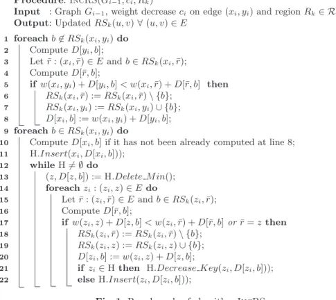
Hence in what follows, we describe how our solution updates Road-Signs. The algorithm is denoted as IncRS and its pseudo-code is given in Figure 1. The algorithm is based on the observation that, when ci occurs, all the shortest
paths which contain (xi, yi) in Gi−1 (i.e. before ci) are shortest paths also in
Gi (i.e. after ci). Therefore, if some boundary node for some region Rk belongs
to RSk(xi, yi) before ci it belongs also to RSk(xi, yi) after ci and no update is
needed for it. However, it could happen that the shortest path from xi to some
boundary node b of Rk in Gi−1 does not contain (xi, yi) but, after the weight
decrease, the new shortest path in Gi contains (xi, yi). In this case, b needs to
be added to RSk(xi, yi) and removed from RSk(xi, w), where (xi, w) is the edge
outgoing xi whose road signs b belongs to. Same arguments can be applied to
the incoming edges of xi, (z, xi): if a boundary node belongs to RSk(z, xi) and
RSk(xi, yi) before ci, then it belongs also to RSk(z, xi) after ci; if a boundary
node b is in RSk(xi, yi) (because it was already in RSk(xi, yi) or because it has
been added to it as a consequence of ci) and it does not belong to RSk(z, xi)
before ci, then it might be added to RSk(z, xi) in the case that the shortest path
from z to b in Gicontains the sub-path (z, xi, yi). We iteratively apply the same
arguments to the other edges of the graph, starting from xi and traversing its
incoming edges. Note that, if at some point of the iteration we find out that the shortest path from a node z to some boundary node b does not decrease, then we do not need to add or remove b to any incoming edge of z. This allows us to reduce the search space of the algorithm.
IncRS works in two phases. In the first phase (lines 1–8) RSk(xi, yi) is updated by possibly adding new boundaries b 6∈ RSk(xi, yi) to it. This phase
is performed for each b 6∈ RSk(xi, yi) separately (line 1). In the pseudo-code,
when needed, we store distances between a node u and a boundary b in data structure D[u, b] and we use an heap H to compute the minimum among the computed distances. Since each boundary node is processed separately, these data structures are overwritten at each computation, hence requiring O(n) space in the worst case. In detail, at lines 2 and 3–4 we compute the distances from yi to b and from node ¯r such that b ∈ RSk(xi,r) to b, respectively. Then, at¯
line 5, we check whether the weight of the path passing through yi is smaller
than that passing through ¯r(that is the shortest path from xi to b in Gi−1). In
the affirmative case, we update the road signs by adding b to RSk(xi, yi) and
removing b from RSk(xi,r) (lines 6–7). Moreover, we store the new distance¯
from xi to b in D[xi, b] (line 8) in order to use it in the next phase. In the
second phase (lines 9–22) the road signs are updated for each b ∈ RSk(xi, yi)
separately. The updating is done by mimicking the Dijkstra’s algorithm, that is by greedily visiting the reverse graph starting from xiand stopping when a node
does not need to update the road signs of its outgoing edges wrt b. At line 11, H is initialized by inserting xi into it using D[xi, b] as key. If b was already in RSk(xi, yi), then D[xi, b] has not been computed at line 8 and hence it is
Procedure: IncRS(Gi
−1, ci, Rk)
Input : Graph Gi−1, weight decrease cion edge (xi, yi) and region Rk∈ R
Output: Updated RSk(u, v) ∀ (u, v) ∈ E
1 foreach b 6∈ RSk(xi, yi) do 2 Compute D[yi, b]; 3 Let ¯r: (xi,¯r) ∈ E and b ∈ RSk(xi,¯r); 4 Compute D[¯r, b]; 5 if w(xi, yi) + D[yi, b] < w(xi,r) + D[¯¯ r, b] then 6 RSk(xi,¯r) := RSk(xi,¯r) \ {b}; 7 RSk(xi, yi) := RSk(xi, yi) ∪ {b}; 8 D[xi, b] := w(xi, yi) + D[yi, b]; 9 foreach b ∈ RSk(xi, yi) do
10 Compute D[xi, b] if it has not been already computed at line 8;
11 H.Insert(xi, D[xi, b])); 12 while H 6= ∅ do 13 (z, D[z, b]) := H.Delete M in(); 14 foreach zi: (zi, z) ∈ E do 15 Let ¯r: (zi,r) ∈ E and b ∈ RS¯ k(zi,r);¯ 16 Compute D[¯r, b]; 17 if w(zi, z) + D[z, b] < w(zi,r) + D[¯¯ r, b] or ¯r= z then 18 RSk(zi,r) := RS¯ k(zi,r) \ {b};¯ 19 RSk(zi, z) := RSk(zi, z) ∪ {b}; 20 D[zi, b] := w(zi, z) + D[z, b];
21 if zi∈ H then H.Decrease Key(zi, D[zi, b]));
22 else H.Insert(zi, D[zi, b]));
Fig. 1. Pseudo-code of algorithm IncRS.
D[z, b] is extracted from H. Then, for each node zi such that (zi, z) ∈ E, at
lines 14–22 we perform the same steps done for xi and (xi, yi): we compute the
distance from ¯r such that b ∈ RSk(zi,r) to b; we check whether the weight of¯
the path from zi to b passing through z is smaller than that passing through ¯r
and, in the affirmative case, we update the road signs by adding b to RSk(zi, z)
and removing it from RSk(zi,r); finally, we store the new distance from z¯ i to b
in D[zi, b] and insert zi into H or decrease its key if it already belongs to H.
The following theorem states the correctness of IncRS.
Theorem 1. Given G = (V, E, w) and a partition R = {R1, R2, . . . , Rr} of V ,
for each (u, v) ∈ E and Rk∈ R, IncRS correctly updates RSk(u, v) and Ak(u, v)
after a weight decrease operation on an edge of G.
Proof. Let us consider a region Rk ∈ R and a weight decrease operation ci
on edge (xi, yi). From Proposition 1, it is enough to show that IncRS correctly
updates RSk(u, v) after ci, for each (u, v) ∈ E. Given an edge (u, v), we denote as
RSk(u, v) and RSk′(u, v) the road-signs of (u, v) before and after ci, respectively.
As ci decreases the weight of (xi, yi), then RSk(xi, yi) ⊆ RS′k(xi, yi),
boundary nodes in RS′
k(xi, yi), that is RSk′(u, v) \ RSk(u, v) ⊆ RSk′(xi, yi) and
RSk(u, v) \ RSk′(u, v) ⊆ RSk′(xi, yi). It follows that phase one (lines 1–8)
cor-rectly updates the road-signs of edges outgoing from xi. The road-signs of the
remaining edges are updated in phase two, whose correctness is shown separately for each boundary node b ∈ RS′
k(xi, yi) and derives from the following facts.
F1 The nodes are extracted from H at line 13 in non-decreasing order of keys. Let us consider two nodes u and v extracted from H at times tu and tv with
keys D[u, b] and D[v, b], respectively. By contradiction, suppose that tu< tvand
D[u, b] > D[v, b]. Since at line 13 the node with the minimum key is extracted, at time tu, D[u, b] was minimum and hence either u has been extracted into
H after tu or its key has been decreased after tu. In both cases, the algorithm passed the test at line 17 which implies that there exists a node v1 and a time
tv1 < tv such that D[v1, b] < D[v, b] < D[u, b], where D[v1, b] is the key of v1
at time tv1 when v1is extracted from H. If we iteratively repeat this arguments
for node v1, we obtain a sequence of nodes v ≡ v0, v1, v2, . . . , vk, where vk≡ xi,
such that, if we denote as D[vj, b] the key of vj when it is extracted from H at
time tvj, then D[vj+1, b] < D[vj, b] and tvj+1 < tvj for each j = 0, 1, . . . k − 1.
For the condition at line 12, one of the nodes in the sequence vj has to belong
to H with key D[vj, b] < D[u, b] at time tu which contradicts the fact that, at
time tu, node u is the node with the minimum key.
F2 A node is extracted from H at line 13 at most once.
Suppose that a node u is extracted from H at two different times t1< t2. Then,
node u has been inserted into H at two different times, denoted as ¯t1 and ¯t2,
when it does not belong to H. It follows that [¯t1, t1] ∩ [¯t2, t2] = ∅. Further, let us
denote as Dt1[u, b] (Dt2[u, b], resp.) the key of u at time ¯t1 (¯t2, resp.) which is
equal to that at time t1 (t2, resp.). Let us consider the two (possibly different)
nodes v1 and v2 which are extracted from H immediately before times ¯t1 and
¯
t2, respectively. Let us analyze the keys extracted from H. At time ¯t1, v1 is
extracted with key D[v1, b], D[u, b] is set to Dt1[u, b] = w(u, v1) + D[v1, b] and
b is added to RSk(u, v1). At time t1, u is extracted with key Dt1[u, b]. At time
¯
t2, v2 is extracted with key D[v2, b], and D[u, b] is set to Dt2[u, b] = w(u, v2) +
D[v2, b], it follows that the test at line 17 returned true and, as b ∈ RSk(u, v1),
w(u, v2) + D[v2, b] < w(u, v1) + D[v1, b]. Hence Dt2[u, b] < Dt1[u, b]. At time t2,
uis extracted with key Dt2[u, b] and, since t1< t2, this contradicts Fact F1.
F3 For each edge (u, v) such that RS′
k(u, v) 6= RSk(u, v), u is inserted into H.
We show a stronger statement that is: if a node changes its distance to b ∈ RS′
k(u, v) it is inserted into H. By contradiction, let us consider the node u such
that: it changes its distance to b, it is not inserted into H, and its distance to b after ci is minimal among the nodes with the same properties. By this last
property, the node v on the shortest path from u to b after ci is inserted into H.
When v is extracted from H, either b belongs to RSk(u, v) or w(u, v) + D[v, b] <
w(u, ¯r) + D[¯r, b], where ¯r is the node such that b ∈ RSk(u, ¯r). In both cases, u
is inserted into H at line 22.
F4When a node u is extracted from H at line 13, for each (u, v) ∈ E, RSk(u, v)
graph n. of nodes n. of edges %mot %nat %reg %urb lux 30 647 75 576 0.55 1.95 14.77 82.71 dnk 469 110 1 090 148 24.02 3.06 0.48 72.45 bel 458 403 1 164 046 22.90 2.92 0.52 73.62 aut 722 512 1 697 902 27.60 5.33 1.71 65.21 esp 695 399 1 868 838 33.22 6.34 1.51 58.87 ned 892 027 2 278 824 0.40 0.56 5.16 93.86 swe 1 546 705 3 484 378 19.54 2.86 0.45 77.10
Table 1. Tested road graphs. 1st col.: the graph; 2nd and 3rd col.s: number of nodes and edges in the graph; 4th–7th col.s: percentage of edges into categories: motorways (mot), national roads (nat), regional roads (reg), and urban streets (urb).
By contradiction, let us consider the first node u whose outgoing edges have wrong road-signs when u is extracted from H. Let us consider the node v such that b ∈ RSk(u, v) when u is extracted, that is v is the node that was extracted
from H immediately before the last time that either u is inserted into H or its key is decreased. As u is the first node whose outgoing edges have wrong road-signs when it is extracted from H, then the road-road-signs of the edges outgoing from v are correctly updated. Moreover, also the road-signs of edges outgoing from w, for each (u, w) ∈ E are correctly updated. In fact two cases may arise: if w changes the road-signs of its outgoing edges then, by Fact F3, it is inserted into H, by facts F1 and F2, it is extracted before u and hence, by hypothesis, it correctly updates the road-signs of its outgoing edges; otherwise the road-signs of its outgoing edges are already correct. In any case, when u is inserted into H the distances used in the test of line 17 are correctly computed and hence the road signs are correctly updated. ¤ From a theoretical point of view, IncRS requires a computational complexity which is, in the worst case, comparable to that of the recomputation from scratch of Arc-Flags. However, IncRS focuses the computation only on the nodes that change shortest paths to a subset of the boundary nodes (and possibly on the neighbors of such nodes). In contrast, the recomputation from scratch computes all the shortest paths from any boundary node to each other node of the network. This difference is difficult to be captured by a worst case analysis and this motivates the experimental study of the next section.
4
Experimental study
In this section, we compare the performances of the incremental algorithm pro-posed in this paper and the decremental algorithm of [3], whose combination is named here DynRS, on fully dynamic sequences of weight change operations against the recomputation from scratch of Arc-Flags. We used the implementa-tion of Arc-Flags of [2]. Furthermore, it has been shown in [10] that the best query performances for Arc-Flags are achieved when partitions are computed by using arc-separator algorithms. For this reason, we used arc-separators obtained
1e+00 1e+01 1e+02 1e+03 1e+04 1e+05
mot nat reg urb
1e+00 1e+01 1e+02 1e+03 1e+04 1e+05 1e+06 1e+07 1e+08
mot nat reg urb
Fig. 2. Speed-up factors of the fully dynamic algorithm for the road network of Sweden, without (left) and with (right) outliers.
by the METIS library [8]. Our experiments are performed on a workstation equipped with a Quad-core 3.60 GHz Intel Xeon X5687 processor, with 12MB of internal cache and 24 GB of main memory. The program has been compiled with GNU g++ compiler 4.4.3 under Linux (kernel 2.6.32).
We consider seven road graphs available from PTV [11] representing the road networks of Luxembourg, Denmark, Belgium, Austria, Spain, Netherlands and Sweden, denoted as lux, dnk, bel, aut, esp, ned and swe, respectively. In each graph, edges are classified into four categories according to their speed limits: motorways (mot), national roads (nat), regional roads (reg) and urban streets (urb). The main characteristics of these graphs are reported in Table 1. We consider fully dynamic sequences of updates simulating disruptions on road networks built as follows. The most significant operation that can occur on a road segment is the increase of a weight, which simulates a delay in the travel time on that segment due, for instance, to a traffic jam. This operation is usually followed by a weight decrease on the same road segment which simulates the restore from the delay. Hence, for each operation in the sequence that increases the weight of an edge (xi, yi) of a quantity γi, there is a corresponding subsequent
operation which decreases the weight of edge (xi, yi) of the same amount γi. We
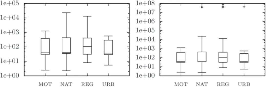
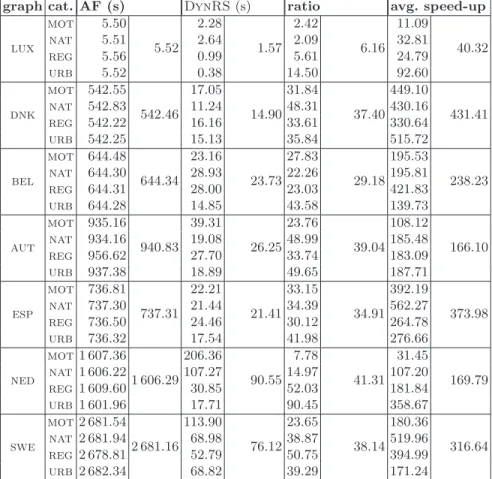
execute, for each graph considered and for each road category, random sequences of 100 weight-change operations as described above. The weight-change amount for each operation is chosen uniformly at random in [25%, 75%] of the weight of the edge involved in that operation. As a performance indicator, we choose the time used by the algorithms to complete a single update during the execution of a sequence. We measure, as speed-up factor, the ratio between the time required by the recomputation from scratch of Arc-Flags and that required by DynRS. The results are reported in Fig. 2–3, and in Table 2.
Fig.s 2 and 3 show two box-plot diagrams representing the values of the speed-up factors obtained for swe and ned. For each category, we represent minimum value, first quartile, median value, third quartile, and maximum value. In both figures, the diagram on the left does not show outlier values while the diagram
1e+00 1e+01 1e+02 1e+03 1e+04
mot nat reg urb
1e+00 1e+01 1e+02 1e+03 1e+04 1e+05 1e+06 1e+07 1e+08
mot nat reg urb
Fig. 3. Speed-up factors of the fully dynamic algorithm for the road network of the Netherlands, without (left) and with (right) outliers.
on the right does. Outlier values occur when DynRS performs much better than Arc-Flags because the number of Road-Signs changed is very small. We consider a test as outlier if the speed-up factor is 1000 times the speed-up factor median value. Even without outliers, the speed-up gained by DynRS is high.
Notice that, in the case of swe (Fig. 2), the speed-up factors are quite similar on the different categories, thus highlighting an independency from categories. This is the typical behavior of road networks, as shown also for bel, dnk, esp and aut in Table 2, where we report the average time of the recomputation from-scratch of Arc-Flags and the average time of DynRS, the average ratios between these quantities and the speed-up factors. The only exceptions are lux and ned, where the percentage of motorways is very low. This is the reason why we highlight the behavior of DynRS on ned in Fig. 3, where the speed-up factor reaches the highest values when update operations occur on urban edges, while it is smaller when they occur on motorway edges. In fact, when an update operation occurs on urban edges, the number of shortest paths that change is small compared to the case that an update operation occurs on motorways edges. This implies that DynRS, which selects the nodes that change such shortest paths and focus the computation only on such nodes, performs better than the recomputation from-scratch of the shortest paths from any boundary node.
We note that, the speed-up factor increases with the size of the network. This can be explained by the fact that, when an edge update operation occurs, it affects only a part of the graph, hence only a subset of the edges in the graph need to update their Arc-Flags or Road-Signs. In most of the cases, this part is small compared to the size of the network and, with high probability, it corresponds to the subnetwork close to the edge increased or closely linked to it. In other words, it is unlike that a traffic jam in a certain part of the network affects the shortest paths of another part which is far or not linked to the first one. Clearly, this fact is more evident when the road network is big. In conclusion, it is evident from Table 2, that DynRS outperforms the recomputation from-scratch by far and that it requires reasonable computational time.
graph cat. AF (s) DynRS(s) ratio avg. speed-up lux mot 5.50 5.52 2.28 1.57 2.42 6.16 11.09 40.32 nat 5.51 2.64 2.09 32.81 reg 5.56 0.99 5.61 24.79 urb 5.52 0.38 14.50 92.60 dnk mot 542.55 542.46 17.05 14.90 31.84 37.40 449.10 431.41 nat 542.83 11.24 48.31 430.16 reg 542.22 16.16 33.61 330.64 urb 542.25 15.13 35.84 515.72 bel mot 644.48 644.34 23.16 23.73 27.83 29.18 195.53 238.23 nat 644.30 28.93 22.26 195.81 reg 644.31 28.00 23.03 421.83 urb 644.28 14.85 43.58 139.73 aut mot 935.16 940.83 39.31 26.25 23.76 39.04 108.12 166.10 nat 934.16 19.08 48.99 185.48 reg 956.62 27.70 33.74 183.09 urb 937.38 18.89 49.65 187.71 esp mot 736.81 737.31 22.21 21.41 33.15 34.91 392.19 373.98 nat 737.30 21.44 34.39 562.27 reg 736.50 24.46 30.12 264.78 urb 736.32 17.54 41.98 276.66 ned mot1 607.36 1 606.29 206.36 90.55 7.78 41.31 31.45 169.79 nat 1 606.22 107.27 14.97 107.20 reg 1 609.60 30.85 52.03 181.84 urb 1 601.96 17.71 90.45 358.67 swe mot2 681.54 2 681.16 113.90 76.12 23.65 38.14 180.36 316.64 nat 2 681.94 68.98 38.87 519.96 reg 2 678.81 52.79 50.75 394.99 urb 2 682.34 68.82 39.29 171.24
Table 2. Avg update times and speed-up factors of DynRS. 1st col.: graph; 2nd col.: category where the weight changes occur; 3rd and 4th col.s: avg computational time for Arc-Flags and DynRS, resp.; 5th col.: ratio between the values of the 3rd and the 4th col.s; 6th col.: avg speed-up factors of DynRS against Arc-Flags.
Regarding the preprocessing phase, in Table 3 we report the computational time and the space occupancy required by Arc-Flags and DynRS. Table 3 shows that, for computing Road-Signs along with Arc-Flags, we need about twice the computational time required for computing only Arc-Flags, which is a small overhead compared to the speed-up gained in the updating phase. The same observation can be done regarding the space occupancy. In fact, Table 3 also shows that the space required for storing both Road-Signs and Arc-Flags is between 1.44 and 3.48 times that required to store only Arc-Flags.
References
1. A. Berger, M. Grimmer, and M. Mller-Hannemann. Fully dynamic speed-up tech-niques for multi-criteria shortest path searches in time-dependent networks. In In
graph reg. AF (s) AF+RS (s) t. ratio AF (B) AF+RS (B) s. ratio lux 64 5.52 11.79 2.14 1 209 216 1 744 531 1.44 dnk 128 542.46 1 104.16 2.04 17 442 368 43 932 508 2.52 bel 128 644.34 1 373.11 2.13 18 624 736 64 759 010 3.48 aut 128 940.83 1 995.93 2.12 27 166 432 78 720 055 2.90 esp 128 737.31 1 446.65 1.96 29 901 408 67 664 666 2.26 ned 128 1 606.29 3 214.34 2.00 36 461 184 64 612 836 1.77 swe 128 2 681.16 5 986.62 2.23 55 750 048 163 151 588 2.93 Table 3. Preprocessing time and space. 1st col.: graph; 2nd col.: number of regions; 3rd col.: preprocessing time, in seconds, of Arc-Flags; 4th col.: preprocessing time, in seconds, of Arc-Flags and Road-Signs; 5th col.: ratio between the values reported in the 4th and the 3rd column; 6th col.: space required, in Bytes, to store Arc-Flags; 7th col.: space required, in Bytes, to store Arc-Flags and Road-Signs; 8th col.: ratio between the values of the 7th and the 6th column.
9th Int. Symposium on Experimental Algorithms (SEA’10), volume 6049 of Lecture Notes in Computer Science, pages 35–46. Springer, 2010.
2. E. Berrettini, G. D’Angelo, and D. Delling. Arc-flags in dynamic graphs. In Proc. of the 9th Workshop on Algorithmic Approaches for Transportation Modeling, Optimization, and Systems (ATMOS 2009). Schloss Dagstuhl, Germany, 2009.
3. G. D’Angelo, D. Frigioni, and C. Vitale. Dynamic arc-flags in road networks. In 10th Int. Symp. on Exp. Algorithms (SEA2011), volume 6630 of Lecture Notes in Computer Science, pages 88–99, 2011.
4. D. Delling, A. V. Goldberg, T. Pajor, and R. F. Werneck. Customizable route planning. In Proc. 10th Int. Symposium on Experimental Algorithms (SEA’11), volume 6630 of Lecture Notes in Computer Science, pages 376–387. Springer, 2011.
5. D. Delling, P. Sanders, D. Schultes, and D. Wagner. Engineering Route Planning Algorithms. In Algorithmics of Large and Complex Networks, volume 5515 of LNCS, pages 117–139. 2009.
6. D. Delling and D. Wagner. Landmark-Based Routing in Dynamic Graphs. In 6th Work. on Exp. Algorithms (WEA’07), volume 4525 of LNCS, pages 52–65, 2007.
7. A. V. Goldberg and C. Harrelson. Computing the Shortest Path: A* Search Meets Graph Theory. In 16th Annual ACM–SIAM Symp. on Discrete Algorithms (SODA’05), pages 156–165, 2005.
8. G. Karypis. METIS - A Family of Multilevel Partitioning Algorithms, 2007.
9. U. Lauther. An extremely fast, exact algorithm for finding shortest paths. Static Networks with Geographical Background, 22:219–230, 2004.
10. R. H. M¨ohring, H. Schilling, B. Sch¨utz, D. Wagner, and T. Willhalm. Partitioning Graphs to Speedup Dijkstra’s Algorithm. ACM J. Exp. Algorithmics, 11:2.8, 2006.
11. PTV AG - Planung Transport Verkehr. http://www.ptv.de, 2008.
12. P. Sanders and D. Schultes. Engineering Highway Hierarchies. In 14th European Symp. on Algorithms (ESA’06), volume 4168 of LNCS, pages 804–816, 2006.
13. P. Sanders and D. Schultes. Dynamic Highway-Node Routing. In 6th Work. on Exp. Algorithms (WEA’07), volume 4525 of LNCS, pages 66–79, 2007.
14. F. Schulz, D. Wagner, and C. Zaroliagis. Using Multi-Level Graphs for Timetable Information in Railway Systems. In 4th Work. on Algorithm Engineering and Experiments (ALENEX’02), volume 2409 of LNCS, pages 43–59, 2002.
15. D. Wagner, T. Willhalm, and C. Zaroliagis. Geometric Containers for Efficient Shortest-Path Computation. ACM J. Exp. Algorithmics, 10:1.3, 2005.