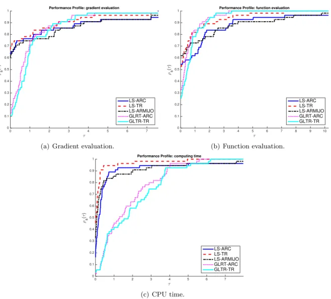
A line-search algorithm inspired by the adaptive cubic regularization framework with a worst-case complexity O(−3/2)
E. Bergou ∗ Y. Diouane† S. Gratton‡ December 4, 2017
Abstract
Adaptive regularized framework using cubics (ARC) has emerged as an alternative to line-search and trust-region for smooth nonconvex optimization, with an optimal complexity amongst second-order methods. In this paper, we propose and analyze the use of a special (iteration dependent) scaled norm in ARC of the formkxkM =
√
x>M xforx∈Rn, where M is a symmetric positive definite matrix satisfying specific secant equation. Within the proposed norm, ARC behaves as a line-search algorithm along the Newton direction, with a special backtracking strategy and acceptability condition. Under appropriate assumptions, the obtained algorithm enjoys the same convergence and complexity properties as ARC, in particular the complexity for finding an approximate first-order stationary point isO(−3/2).
Furthermore, using the same scaled norm in the trust-region framework, we have derived a second line-search algorithm. The good potential of the obtained algorithms is showed on a set of large scale optimization problems.
Keywords: Nonlinear optimization, unconstrained optimization, line-search methods, adaptive regularized framework using cubics, trust-region methods, worst-case complexity.
1 Introduction
We consider the following unconstrained optimization problem:
x∈minRn
f(x), (1)
where f :Rn→ Ris a given smooth function known as the objective function. Classical itera- tive methods for solving (1) are trust-region (TR) [8, 19] and line-search (LS) [10] algorithms.
Recently, the use of cubic regularization has been first investigated by Nesterov and Polyak [17]
and then Cartis et al [5] propose a generalization to an adaptive regularized framework using cubics (ARC).
∗MaIAGE, INRA, Universit´e Paris-Saclay, 78350 Jouy-en-Josas, France ([email protected]).
†Institut Sup´erieur de l’A´eronautique et de l’Espace (ISAE-SUPAERO), Universit´e de Toulouse, 31055 Toulouse Cedex 4, France ([email protected]).
‡INP-ENSEEIHT, Universit´e de Toulouse, 31071 Toulouse Cedex 7, France ([email protected]).
The worst-case evaluation complexity of finding an -approximate first-order critical point using TR or LS methods is shown to be computed in at most O(−2) function or gradient evaluations, where∈(0,1) is a user-defined accuracy threshold on the gradient norm [16, 14, 7].
ARC takes at mostO(−3/2) function or gradient evaluations to reduce the gradient norm below , and thus it is improving substantially the worst-case complexity over the classical TR/LS methods [4]. Such complexity bound can be improved using higher order regularized models, we refer the reader for instance to the references [2, 6].
More recently, a non-standard TR method [9] is proposed with the same worst-case complex- ity bound as ARC. It is proved also that the same worst-case complexityO(−3/2) can be achieved by mean of a specific variable-norm in a TR method [15] or using quadratic-regularization [3]. All previous approaches use a cubic sufficient-descent condition instead of the more usual predicted- reduction based descent. Generally, they need to solve more than one linear system in sequence at each outer iteration, this makes the computational cost per iteration expensive (By outer iteration, one means the sequence of the iterates generated by the the algorithm). In this work, under appropriate assumptions, we will derive an algorithm with the same worst-case complexity of O(−3/2) without imposing any cubic sufficient-descent condition on the objective function and requiring only to solve (approximately) one linear system per iteration to get a trial point.
In [1], it has been shown how to use the so-called energy norm in the ARC/TR framework when a symmetric positive definite (SPD) approximation of the objective function Hessian is available. Within the energy norm, ARC/TR methods behave as LS algorithms along the Newton direction, with a special backtracking strategy and an acceptability condition in the spirit of ARC/TR methods. As far as the model of the objective function is convex (i.e., the approximate Hessian is SPD), in [1] we developed a methodology to make ARC behaves as an LS algorithm and showed that the resulting algorithm enjoys the same convergence and complexity analysis properties as ARC, in particular the first-order complexity bound of O(−3/2). In the complexity analysis of ARC method [4], it is required that the Hessian approximation has to approximate accurately enough the true Hessian (see [4, Assumption AM.4]), obtaining such convex approximation may be out of reach when handling nonconvex optimization. This paper generalizes the proposed methodology in [1] to handle nonconvex models.
In this paper, we show that by using a special scaled norm the computational cost of the ARC subproblem is nearly the same as solving a linear system. In fact, the proposed approach consists of the use of a scaled norm to define the regularization term in ARC subproblem. The chosen scaled norm is of the formkxkM =
√
x>M xforx∈Rn, where M is an SPD matrix that satisfies a specific secant equation. At each iteration we choose a possible different matrix M. (So, M =Mk where the subscript k is the outer iteration index). Assuming that the Newton direction is not orthogonal with the gradient off at the current iterate, the specific choice ofM renders the ARC subproblem solution collinear with the Newton step and hence leads to an LS algorithm, along the Newton direction. The obtained LS algorithm enjoys the same convergence and worst-case complexity results as ARC method. Additionally, using subspace methods, we also consider a large-scale variant for the case where matrix factorizations are not affordable, implying that only iterative methods for computing a trial step can be used.
Compared to ARC (when using the`2-norm to define the regularization term in the subprob- lem), the dominant computational cost (regardless the function evaluation cost) of the resulting algorithm is mainly the cost of successful iterations. In fact, using the proposed scaled norm, the cost of the subproblem solution for unsuccessful iterations is getting inexpensive and requires only an update of a scalar.
An interesting feature of the obtained LS algorithm is the strategy of proceeding line search along the Newton direction which leads to the optimal complexity of ARC (independently from the convexity of the quadratic approximation of f). This is not the typical strategy that one may follow for defining a line-search method, especially when f is concave around the current iterate. The reason of using the Newton direction rather than another descent direction is to keep the worst case complexity bound of order −3/2. In fact, minimizing along the Newton direction ensures the existence of a scaled norm (which is uniformly equivalent to the Euclidean norm) such that a stationary point of the cubic model can be found along the same direction.
Hence, the convergence and complexity analysis can be deduced directly from ARC algorithm.
With a different direction, one is not sure about the existence of a scaled norm with the desired properties.
The proposed analysis of the obtained LS algorithm assumes that the Newton direction is not orthogonal with the gradient off during the minimization process. To satisfy such assumption, we propose to check first if there exists an approximate of the Newton direction (among all the iterates generated using a subspace method) which is not orthogonal with the gradient and that satisfies the desired properties. If the subspace method reaches the exact solution and the assumption is still violated, we avoid such assumption by minimizing the cubic model using the `2-norm until a successful outer iteration is found. This procedure is included in the final LS algorithm. We note that in our numerical tests the latter restoration procedure was never activated, we believe from the practical point of view that such assumption is not very restrictive.
Similar analysis is applied to the TR framework, where using the same scaled norm (as in ARC) we show that TR method behaves as an LS algorithm. Numerical illustrations (over a test set of large scale optimization problems) are given in order to assess the efficiency of the obtained LS algorithms.
We organize this paper as follows. In Section 2, we introduce the ARC method using a general scaled norm. Section 3 analyses the minimization of the cubic model and discusses the choice of the scaled norm that simplifies solving the ARC subproblem. Section 4 derives the obtained LS algorithm on the base of ARC (when the proposed scaled norm is used) and discusses how the iteration dependentM-norm can be chosen uniformly equivalent to the Euclidean norm. We end the section by stating the necessary stopping criteria that is needed to maintain the complexity of ARC when the subproblem is solved iteratively. Similarly to ARC and using the same scaled norm, an LS algorithm in the spirit of TR algorithm is proposed in Section 5. Numerical tests are illustrated and discussed in Section 6. Conclusions and future improvements are given in Section 7.
Throughout this paperk · k will denote the vector or matrix`2-norm. k.kM will denote the scaled norm which is of the form kxkM =
√
x>M x for x ∈ Rn and where M is a given SPD matrix. We denote also by sgn(α) the sign of a real α.
2 The ARC framework
At a given iterate xk, we define mQk :Rn→R as an approximate second-order Taylor approxi- mation of the objective function f around xk, i.e.,
mQk(s) = f(xk) +s>gk+1
2s>Bks, (2)
where gk =∇f(xk) is the gradient off at the current iterate xk, and Bk is a symmetric local approximation of the Hessian off atxk. For ARC [5], the trial stepskapproximates the global minimizer of the cubic model mCk(s) =mQk(s) +13σkksk3M
k, i.e., sARCk ≈arg min
s∈Rn
mCk(s), (3)
where Mk is a positive definite matrix, and σk>0 is a dynamic positive parameter that might be regarded as the reciprocal of the TR radius in TR algorithms (see [5]). The parameter σk is taking into account the agreement between the objective function f and the model mCk. To decide whether the trial step is acceptable or not a ratio between the actual reduction and the predicted reduction is computed, as follows:
ρk = f(xk)−f(xk+sARCk )
f(xk)−mQk(sARCk ) . (4) For a given scalar 0 < η < 1, the kth outer iteration will be said successful if ρk ≥ η, and unsuccessful otherwise. For all successful iterations we set xk+1 = xk+sARCk ; otherwise the current iterate is kept unchangedxk+1=xk. We note that, unlike the original ARC [5, 4] where the cubic model is used to evaluate the denominator in (4), in the nowadays works related to ARC, only the quadratic approximation mQk(sARCk ) is used in the comparison with the actual value of f without the regularization parameter (see [2] for instance). Algorithm 1 gives a detailed description of ARC.
Algorithm 1: ARC algorithm.
Data: select an initial pointx0 and the constant 0< η <1. Set the initial regularization σ0>0, and the constants 0< ν1 ≤1< ν2.
fork= 1,2, . . . do
Step 1: compute the gradientgk and an approximated Hessian Bk;
Step 2: compute the stepsARCk as an approximate solution of (3) such that
mCk(sARCk ) ≤ mCk(sCauchyk ) (5) wheresCauchyk =−δCauchyk gk andδCauchyk = arg min
t>0 mCk(−tgk) ; Step 3: if ρk ≥η then
setxk+1=xk+sARCk and σk+1 =ν1σk; else
setxk+1=xk and σk+1 =ν2σk; end
end
The Cauchy step sCauchyk , defined in Step 2 of Algorithm 1, is computationally inexpensive compared to the computational cost of the global minimizer ofmCk. The condition (5) onsARCk is sufficient for ensuring global convergence of ARC to first-order critical points. Under appropriate assumptions, convergence results of Algorithm 1 can be found in [5, 2]. Moreover, in this case, the algorithm ensures a function-evaluation complexity bound of order −2 to guarantee
kgkk ≤ , (6)
where >0 is a pre-defined constant.
IfBkis set to be equal to the exact Hessian of the problem in Step 1 of Algorithm 1, one can improve the function-evaluation complexity to be of the order of −3/2 for ARC algorithm by imposing, in addition to the Cauchy decrease, another termination condition on the computation of the trial stepsARCk (see [4, 2]). Such a termination condition is of the form
k∇mCk(sARCk )k ≤ ζksARCk k2, (7) where ζ >0 is a given constant chosen at the start of the algorithm.
When only an approximation of the Hessian is available in Step 1 of Algorithm 1, an ad- ditional condition has to be imposed on the Hessian approximation Bk in order to ensure an optimal complexity of order −3/2. Such condition is often considered as (see [4, Assumption AM.4]):
k(∇2f(xk)−Bk)sARCk k ≤CksARCk k2 (8) for all k≥0 and for some constantC >0.
From now on, we will assume that first-order stationarity is not reached yet, meaning that the gradient of the objective function is non null at the current iteration k (i.e.,gk6= 0).
3 On the cubic model minimization
In this section, we will mostly focus on the solution of the subproblem (3) for a given outer iteration k. Thus the subscript kwill be dropped to keep the notations simple. In a precedent work [1], when the matrix B is assumed to be positive definite, we showed that the minimizer sARC of the cubic model defined in (3) is getting collinear with the Quasi-Newton direction (−B−1g) when the matrixM is set to be equal to B. In this section we generalize our proposed approach to cover the case where the linear system Bs = −g admits a solution and B is not necessarily SPD. We will explicit the condition to impose on the matrix M in order to get the solution of the ARC subproblem at a modest computational cost.
3.1 Exact solution of the ARC subproblem
For the purpose of this subsection, the vectorsQ will denote an exact solution ofBs=−gwhen it exists (i.e., sQ corresponds to a stationary point ofmQ). Moreover, assuming that sQ is not orthogonal with the gradientg, letdNdenotes a scaled Quasi-Newton direction, i.e.,dN=− sQ
g>sQ. For the sake of simplicity, in what comes next, we shall refer to dN as the Newton direction.
Note that such direction is a descent direction for the objective function f (i.e. g>dN <0). In this subsection, we state our precise assumption formally as follows:
Assumption 3.1 The model mQ admits a stationary point sQ such as |g>sQ| ≥ dkgkksQk where d>0 is a pre-defined positive constant.
When such assumption is violated, in Section 4, we explain our proposed approach to restore such assumption in the final algorithm (see Algorithm 2).
In what comes next, we definesARCN as the Newton-like step associated with the minimization of the cubic modelmC:
sARCN =αNdN, where αN = arg min
t>0 mCk(tdN). (9)
The next theorem gives the explicit form of sARCN .
Theorem 3.1 Let Assumption 3.1 hold. The Newton-like step (9) is given by:
sARCN = δNsQ, where δN= 2 1−sgn(g>sQ)
r
1 + 4σks|g>QskQ3M|
. (10)
Proof. Indeed, for all t >0, one has mC(tdN)−mC(0) = tg>dN+t2
2[dN]>[BdN]>+σt3
3 kdNk3M =−t− 1 g>sQ
t2
2 +σksQk3M
|g>sQ|3 t3
3. We compute the value of the parametert at which the unique minimizer of the above function is attained. Let αN denotes this optimal parameter. Taking the derivative of (11) with respect tot and equating the result to zero, one gets
0 = −1− 1
g>sQαN +σksQk3M
|g>sQ|3 (αN)2, (11) and thus, since αN >0,
αN =
1 g>sQ +
r 1
g>sQ
2
+ 4σks|g>QsQk3M|3
2σks|g>QsQk3M|3
= 2g>sQ
−1 + sgn(g>sQ) r
1 + 4σks|g>QskQ3M|
.
Hence,sARCN =δNsQ, where δNARC= 2
1−sgn(g>sQ) r
1+4σksQk
3 M
|g>sQ|
.
In general, the matrixM can be chosen arbitrarily as long as it is an SPD matrix. Our goal, in this paper, is to determine how we can choose the matrix M so that the Newton-like step sARCN becomes a stationary point of subproblem (3). The following theorem gives explicitly the necessary and sufficient condition on the matrixM to reach this aim.
Theorem 3.2 Let Assumption 3.1 hold. The stepsARCN is a stationary point for the subproblem (3) if and only if there exists θ >0 such that M sQ = g>θsQg. Note that θ=ksQk2M.
Proof. Indeed, if we suppose that the step sARCN is a stationary point of the subproblem (3), this means that
∇smC(sARCN ) = g+BsARCN +σksARCN kMM sARCN = 0, (12) In another hand, sARCN = αNdN where dN = −g>sQsQ and αN > 0 solution of −1− g>1sQαN +
σksQk3M
|g>sQ|3 (αN)2= 0. Hence, we obtain that
0 = ∇smC(sARCN ) =g+ αN
g>sQg−σ(αN)2 ksQkM
|g>sQ| M sQ g>sQ
=
1 + αN g>sQ
g−
σksQk3M
|g>sQ|3 (αN)2 g>sQ ksQk2MM sQ
=
σksQk3M
|g>sQ|3 (αN)2 g− g>sQ ksQk2MM sQ
.
Equivalently, we conclude that M sQ = g>θsQgwhere θ=ksQk2M >0.
The key condition to ensure that the ARC subproblem stationary point is equal to the Newton-like step sARCN , is the choice of the matrix M which satisfies the following secant-like equationM sQ= g>θsQgfor a givenθ >0. The existence of such matrixM is not problematic as far as Assumption 3.1 holds. In fact, Theorem 4.1 explicits a range ofθ >0 for which the matrix M exists. Note that in the formula of sARCN such matrix is used only through the computation of the M-norm of sQ. Therefore an explicit formula of the matrix M is not needed, and only the value ofθ=ksQk2M suffices for the computations.
When the matrixM satisfies the desired properties (as in Theorem 3.2), one is ensured that sARCN is a stationary point for the modelmC and hence condition (7) is automatically satisfied.
However, in addition to such condition, ARC algorithm imposes on the approximate step also to satisfy the Cauchy decrease condition (5) for a givenσ. The latter condition is not guaranteed by sARCN as the modelmC may be non-convex. In the next theorem, we show that for a sufficiently largeσ,sARCN is getting the global minimizer of mC and thus satisfying the Cauchy decrease is not an issue anymore.
Theorem 3.3 Let Assumption 3.1 hold. LetM be an SPD matrix which satisfiesM sQ= g>θsQg for a fixed θ >0. If the matrix B+σksARCN kMM is positive definite, then the step sARCN is the unique minimizer for the subproblem (3).
Proof. Indeed, using [8, Theorem 3.1], we have that, for a given vector s∗, it is a global minimizer ofmC if and only if it satisfies
(B+λ∗M)s∗ =−g
where B +λ∗M is positive semidefinite matrix and λ∗ = σks∗kM. Moreover, if B +λ∗M is positive definite,s∗ is unique.
SinceM sQ= g>θsQg, by applying Theorem 3.2, we see that (B+λNM)sARCN =−g
withλN =σksARCN kM. Thus, if we assume thatB+λNM is positive definite matrix, thensARCN is the unique global minimizer of the subproblem (3).
Theorem 3.3 states that the stepsARCN is the global minimizer of the cubic modelmC as far as the matrix B+λNM is positive definite, whereλN =σksARCN kM. Note that
λN = σksARCN kM = 2σksQkM
1−sgn(g>sQ) r
1 + 4σks|g>QskQ3M|
→+∞ asσ → ∞.
Thus, sinceM is an SPD matrix and the regularization parameterσis increased for unsuccessful iterations in Algorithm 1, the positive definiteness of matrixB+λNM is guaranteed after finitely many unsuccessful iterations. In other words, one would have insurance that sARCN will satisfy the Cauchy decrease after a certain number of unsuccessful iterations.
Another important practical consequence of Theorem 3.3 is that solving exactly the ARC subproblem amounts to computing the solution of the linear system Bs = −g and evaluating the scalar in (10). This means that solving the subproblem, while varying the value of σ,
is inexpensive once the solution of Bs = −g is found. This remark will be essential when considering unsuccessful steps in the overall optimization algorithm. Another consequence is that the subproblem solution can be obtained using a direct method if the matrix B is not too large. Typically, one can use the LDLT factorization to solve this linear system. In the next section we consider the case where Bs=−g is solved iteratively.
3.2 Approximate solution using subspace methods
For large scale optimization problems, computing sQ can be prohibitively computationally ex- pensive. We will show that it will be possible to relax this requirement by letting the step sQ be only an approximation of the exact solution.
For an approximate solution, as far as the global convergence of Algorithm 1 is concerned, all what we need is that the solution of the subproblem (3) yields a decrease in the cubic model which is as good as a the Cauchy decrease as emphasized in (5). In practice, a version of Algorithm 1 solely based on the Cauchy step would suffer from the same drawbacks as the steepest descent algorithm on ill-conditioned problems and faster convergence can be expected if the matrix B influences also the minimization direction. The main idea consists of achieving a further decrease on the cubic model (better that the Cauchy decrease) by projection onto a sequence of embedded Krylov subspaces. We now show how to use a similar idea to compute a solution of the subproblem that is computationally cheap and yields the global convergence of Algorithm 1.
A classical way to approximate the exact solutionsQis by using subspace methods (typically a Krylov subspace method). For that, let Li be a subspace of Rn and l its dimension. Let Qi denotes ann×lmatrix whose columns form a basis of Li. Thus for alls∈ Li, we haves=Qiz, for some z ∈Rl. We will denote by [sQ]i an exact stationary point of the model function mQ over the subspace Li (when it exists)). We define [sARCN ]i as the projection, onto the subspace Li, of the step sARCN associated with the subproblem (3), that is [sARCN ]i = QizN where zN is the Newton-like step associated to the following reduced subproblem:
min
z∈Rl
f(x) +z>Q>i g+1
2z>Q>i BQiz+1 3σkzk3
Q>iM Qi. (13) We update Assumption 3.1 in this subsection as follows:
Assumption 3.2 The model mQ admits a stationary point [sQ]i over the subspace Li such as
|g>[sQ]i| ≥dkgkk[sQ]ik where d>0 is a pre-defined positive constant.
As already mentioned in the exact case, a procedure to restore the violation of such assumption will be included in the final algorithm (see Algorithm 2).
We will now give the extension of the results shown in the previous subsection (the exact case). The next two theorems are the extension of Theorems 3.1 and 3.2 in the inexact case.
Theorem 3.4 Let Assumption 3.2 hold. Then one has
[sARCN ]i = [δN]i[sQ]i where [δN]i = 2 1−sgn(g>[sQ]i)
r
1 + 4σk[s|g>Q[s]Qik]i3M|
. (14)
Proof. Indeed, one has [sARCN ]i = QizN, where zN is the Newton-like step associated to the reduced subproblem (13). Hence by applying Theorem 3.1 to the reduced subproblem (13), it follows that
zN = [δN]izQ where [δN]i = 2 1−sgn((Q>i g)>zQ)
s 1 + 4
σkzQk3
Q>
iM Qi
|(Q>ig)>zQ|
,
where zQ is a stationary point of the quadratic part of the minimized model in (13). Thus, by substitutingzN in the formula [sARCN ]i =QizN, one gets
[sARCN ]i = Qi
2 1−sgn((Q>i g)>zQ)
s 1 + 4
σkzQk3
Q>
i M Qi
|Q>i g)>zQ|
zQ
= 2
1−sgn(g>QizQ) r
1 + 4σkQ|g>iQziQzkQ3M|
QizQ= 2
1−sgn(g>[sQ]i) r
1 + 4σk[s|g>Q[s]Qik]i3M|
[sQ]i.
Theorem 3.5 Let Assumption 3.2 hold. The step [sARCN ]i is a stationary point for the sub- problem (3) over the subspace Li if and only if there exists θ > 0 such that M satisfies M[sQ]i = g>[sθQ]ig .
Proof. The proof is similar to the proof of Theorem 3.2 by considering [sQ]i instead ofsQ. As in the exact case, the key assumption to ensure that, the step [sARCN ]i is a stationary point of (13), is the use of theM-norm whereM is satisfying the following condition: M[sQ]i =
θ
g>[sQ]ig, for a given θ >0. Under Assumption 3.2, the existence of such matrixM is addressed in Theorem 4.1. Again we note that only θis needed for the computation of the desired step.
Similarly to the exact case one can deduce the following result on the optimality of [sARCN ]i
over the subspace Li.
Theorem 3.6 Let Assumption 3.2 hold. Let M be an SPD matrix which satisfies M[sQ]i =
θ
g>[sQ]ig for a fixedθ >0. If the matrixQ>i (B+σk[sARCN ]ikMM)Qi is positive definite, then the step [sARCN ]i is the unique minimizer of the subproblem (3) over the subspace Li.
Proof. Indeed, one has M[sQ]i = g>[sθQ]ig meaning that Q>i M QizQ = θ
(Q>ig)>zQQ>i g. Hence, if we suppose that the matrix Q>i (B +λNM)Qi is positive definite, by applying Theorem 3.2 to the reduced subproblem (13), we see that the step zN is the unique global minimizer of the subproblem (13). We conclude that [sARCN ]i =QizN is the global minimizer of the subproblem (3) over the subspace Li.
Note that, when the growing subspaces Li reach the whole spaceRn, the subspace approx- imation (in exact arithmetics) gives the exact solution of the linear system. On the base of this remark, from now on, we will consider that sQ is computed using a subspace method as described in Subsection 3.2.
4 ARC algorithm using a specific M-norm
In this section, using the proposed M-norm, we show that ARC framework (Algorithm 1) behaves as an LS algorithm. For the sake of clarity, the subscript k is reused to indicate the outer iteration index all over our analysis. In the sequel,sQk will denote an approximate solution of the linear system Bks=−gk when it exists.
Under Assumption 3.2 and given an SPD matrix Mk such that MksQk = θk
gk>sQkgk. By using the Mk-norm in the definition of the cubic model mCk, an approximate stationary point of the subproblem (3) is of the form
sARCk = δksQk, where δk = 2 1−sgn(g>ksQk)
r
1 + 4σkks
Q kk3
Mk
|g>ksQk|
. (15)
Moreover, on the base of Theorem 3.6 and using the update mechanism ofσk in the algorithm, one can guarantee that, after a finite number of unsuccessful iterations, the approximate solution sARCk will satisfy the Cauchy decrease condition (5) as it will approach the global minimum of the cubic model mCk.
For unsuccessful iterations in Algorithm 1, it is required only to update the value of σk
while the current step direction is kept unchanged. Hence, the approximate solutions of the subproblem given by (15) can be obtained only by updating the step-sizeδk. This means that the computational cost ofunsuccessfuliterations is getting cheap compared to solving subproblem as required by ARC when the Euclidean norm is used (see e.g. [5]). As a consequence, the use of the specific proposedMk-norm in Algorithm 1 leads to a new formulation of ARC algorithm where the dominant computational cost is the cost of successful iterations. With such choice of the matrixMk, ARC algorithm behaves as an LS method with a specific backtracking strategy and an acceptance criteria in the sprite of ARC algorithm. The trial step is of the formsARCk =δksQk where the step lengthδk>0 is chosen such as
ρk= f(xk)−f(xk+sARCk ) f(xk)−mQk(sARCk )
≥η and mCk(sARCk )≤mCk(sCauchyk ), (16) or, equivalently,
f(xk+δksQk)≤f(xk) +η
δkgk>sQk +δk2
2[sQk]>BksQk
and mCk(δksQk)≤mCk(−δCauchyk gk).
The step lengths δk and δkCauchy are computed respectively as follows:
δk = 2
1−sgn(g>ksQk) r
1 + 4σkks
Q kk3
Mk
|g>ksQk|
, (17)
and
δkCauchy = 2
g>kBkgk
kgkk2 +
r g>
kBkgk
kgkk2
2
+ 4σkkgkk
3 Mk
kgkk2
(18)