On the use of the energy norm in trust-region and adaptive cubic regularization subproblems

On the use of the energy norm in trust-region and adaptive cubic regularization subproblems

E. Bergou

Y. Diouane

S. Gratton

March 6, 2017

Abstract

We consider solving unconstrained optimization problems by means of two popular glob- alization techniques: trust-region (TR) algorithms and adaptive regularized framework using cubics (ARC). Both techniques require the solution of a so-called “subproblem” in which a trial step is computed by solving an optimization problem involving an approximation of the objective function, called “the model”. The latter is supposed to be adequate in a neigh- borhood of the current iterate. In this paper, we address an important practical question related with the choice of the norm for defining the neighborhood. More precisely, assuming here that the HessianB of the model is symmetric positive definite, we propose the use of the so-called “energy norm” – defined by kxkB =√

x^TBxfor allx∈Rⁿ – in both TR and ARC techniques. We show that the use of this norm induces remarkable relations between the trial step of both methods that can be used to obtain efficient practical algorithms. We furthermore consider the use of truncated Krylov subspace methods to obtain an approxi- mate trial step for large scale optimization. Within the energy norm, we obtain line search algorithms along the Newton direction, with a special backtracking strategy and an accept- ability condition in the spirit of TR/ARC methods. The new line search algorithm, derived by ARC, enjoys a worst-case iteration complexity ofO(^−3/2). We show the good potential of the energy norm on a set of numerical experiments.

Keywords: Nonlinear optimization, unconstrained optimization, trust-region algorithm, adaptive regularized framework using cubics, line search algorithm, energy norm, Krylov subspace methods,

conjugate gradient.

1 Introduction

In this paper, we consider the following unconstrained optimization problem:

x∈

min

f(x), (1)

where f :

is a given smooth function. We propose to solve (1) by means of trust-region (TR) methods [7] or an adaptive regularized framework using cubics (ARC) [6]. In recent years,

∗MaIAGE, INRA, Universit´e Paris-Saclay, 78350 Jouy-en-Josas, France ([email protected]).

†Institut Sup´erieur de l’A´eronautique et de l’Espace (ISAE-SUPAERO), Universit´e de Toulouse, 31055 Toulouse Cedex 4, France ([email protected]).

‡INP-ENSEEIHT, Universit´e de Toulouse, 31071 Toulouse Cedex 7, France ([email protected]).

there has been a constant interest in the TR techniques [7, 11, 9], while ARC algorithms for unconstrained optimization enjoy a growing interest [3, 6, 5, 16, 14, 4]. The key principle of these two approaches is the (possibly iterative) minimization of objective function models (often, but not always, quadratic or cubic). During such minimization process, a control of the step length is used either trough an explicit constraint formulation or through a specific penalization term; that minimization stage is known as the “subproblem”. Both TR and ARC frameworks can also be seen as regularization techniques as they control and impose restrictions on a certain parameter (a TR radius or a regularization parameter). TR algorithms are well established and studied, see [7] and references therein, whereas ARC methods are relatively newer and exhibit good performance in terms of global and local convergence properties as we briefly describe now.

Numerical experiments indicate that ARC algorithms can be competitive with TR approaches when solving small-scale problems [6]. ARC algorithms are also famous since they improve substantially the worst-case iteration and gradient evaluation complexity over the classical TR methods [5]. Such improvement has been recently extended to modified TR methods [9] where a specific step update mechanism is proposed. The proposed TR algorithm exhibits the same worst-case complexity bound as ARC algorithms and enjoys the same convergence properties (fast local and global convergence) as the classical TR methods.

For both frameworks, the trial step from one iterate to the next is approximated by min- imizing a given model of the objective function while the next iterate is maintained in a pre- specified neighborhood of the current iterate. An important practical aspect of TR and ARC techniques is on the use of an appropriate description of the neighborhood. In this paper, we focus on the neighborhoods defined as spheres for some scaled versions of the Euclidean norm, i.e.

=

√

x

M x where M is a symmetric positive definite (SPD) matrix. Under such consideration, approximating the subproblem solution requires (approximately) solving a non-linear system, derived from the optimality conditions, by applying a zero-finding solver to the so-called “secular equation” [7]. Practical approaches to get an approximate solution are proposed in [7, 4, 6, 11], where the solution of the secular equation is typically approximated over specific evolving subspaces using Krylov methods. The main drawback of such approaches is there expensive computational cost as they may require solving multiple linear systems in sequence.

Our approach for choosing M is related to ideas developed, for instance, when solving infinite-

dimensional linear problems arising in elliptic partial differential equations. In fact, it is common

to recourse to iterative techniques for solving the corresponding linear systems after discretiza-

tion. In this setting, finding a sound stopping criterion is essential to overcome both over- and

under- solving the regarded problem, i.e. appropriately balance the error due to the truncation

of the iterative solver and the discretization error. It can be shown that it is theoretically nat-

ural and practically relevant to work with the scaled Euclidean norm where M is chosen as the

matrix of the linear system itself [2, 1]. For optimization problems, the use of the absolute-value

of the Hessian (that corresponds to the energy norm in the case of a positive definite Hessian)

to define the trust region in the TR algorithms was proposed in [7, Section 7.7.1] as “the ideal

trust region” that reflects the proper scaling of the underlying problem. For a large scale indef-

inite Hessian, computing the absolute-value is certainly a computationally expensive task. This

means that for large scale optimization problems the use of the absolute-value energy norm can

be seen as out of reach, and was not further considered in [7]. In this paper, we investigate the

use of the energy norm instead of a general scaled norm for both the TR and ARC algorithms in

the situation where the Hessian of the model is SPD, which we believe is common. To mention

only one widespread application, it occurs when a Gauss-Newton approach is used for solving nonlinear least-squares problems.

In this paper we show that, for locally convex model in TR/ARC framework, the compu- tational cost of the associated subproblem is nearly the same as solving a linear system (i.e., approximating a minimizer of the associated quadratic model), and does not involve nonlinear iterations. We also consider a large-scale variant for the case where matrix factorizations are not affordable, implying that only iterative methods for computing a trial step can be used. In this case, we propose a truncated Krylov subspace method for the subproblem. Using our subprob- lem solvers, we also consider the performance of the overall unconstrained optimization solver and show that the energy norm may produce much better results than a standard Euclidean norm based algorithm. Most notably, our approach is very economical because the dominant computational cost of our TR/ARC algorithms is mainly the cost of successful iterations in the TR/ARC algorithms, solving the subproblem for unsuccessful iterations being straight-forward and inexpensive. The proposed approaches are in practice line search algorithms along the New- ton direction, with a special backtracking strategy and an acceptability condition in the spirit of TR/ARC methods. We show that the proposed line search approach, derived by the ARC framework, enjoys a worst-case iteration complexity of

).

The outline of this paper is as follows. In Section 2 we recall a unified framework for uncon- strained optimization gathering both TR algorithms and the ARC approaches and assuming a general scaled norm is used for the step size control. In Section 3, we present closed formulas for the solution of the subproblem when the energy norm is considered, and propose both direct and iterative scheme for computing it. In Section 4 we derive the overall unconstrained optimization algorithm and discuss possible stopping criteria to maintain the complexity of TR and ARC when the subproblem is solved iteratively. In Section 5, preliminary numerical experiments with basic implementations are presented that show the good behavior of our energy norm algorithm.

Finally, in Section 6 we draw some perspectives and conclusions.

2 TR/ARC algorithms

In this section, we describe the subproblem that occurs in the k

iteration when solving the optimization problem (1) in both the TR algorithms (e.g., [7]) and ARC algorithms (e.g., [6]).

Formally in a basic TR algorithm, one computes a trial step s

by approximately solving

s∈

min

f (x

) + s

g

+

s

B

s = m

(s) (2) s. t.

∆

,

where ∆

> 0 is known as the TR radius, g

=

) is the gradient of f at the current iterate x

, and B

is a symmetric approximation to the local Hessian of f at the point x

. The scaled norm

may vary along the iterations and M

is a symmetric positive definite matrix.

Once the trial step s

is determined, the objective function is computed at x

+ s

and

compared with the value predicted by the model at this point. If the model value predicts

sufficiently well the objective function, the trial point x

+ s

will be accepted and the TR is

eventually expanded. If the model turns out to predict poorly the objective function, the trial

point is rejected and the TR is contracted. For a basic ARC algorithm, the trial step s

is

computed as an approximate minimizer of a cubic model m

: s

= arg min

s∈Rⁿ

m

(s) = m

(s) + 1

3 σ

k

, (3)

where σ

> 0 is a dynamic positive parameter that more or less plays the same role as the inverse of the TR radius (see [6]). Similarly to TR algorithms, the update of the parameter σ

takes into account the agreement between the objective function f and the model m

. The parameter σ

and the current iterate are updated following similar principles as those used for

∆

and x

in the TR methods. More formally, for both frameworks, a ratio between the actual reduction and the predicted reduction plays an important role to decide whether the trial step is acceptable or not. In the TR case, the ratio is of the following form:

ρ

= f (x

)

f (x

+ s

)

f (x

)

m

(s

) , (4) and in the adaptive cubic regularization case is of the form

ρ

= f (x

)

f (x

+ s

)

f (x

)

m

(s

) . (5) To keep the notation simple, and unless it introduces some ambiguity, we will use ρ

for both ρ

and ρ

. For a given scalars 0 < η

η

< 1, the k

iteration will be said very successful if ρ

η

, successful if ρ

[η

, η

), and unsuccessful otherwise. In all successful iterations we set x

= x

+ s

; otherwise the current iterate is kept unchanged x

= x

. Algorithm 1 gives a detailed description of both algorithms (TR and ARC frameworks). The generic name

‘ALGO’ stands either for ‘TR’ or ‘ARC’ in the sequel.

For the purpose of this paper, we will assume that the approximate Hessian matrix B

is positive definite for all iterations.

Assumption 2.1 For all k, the approximate Hessian matrix B

of the model is symmetric positive definite.

To ensure the global convergence of Algorithm 1, the trial step is required to provide a decrease greater than or equal to the reduction attained by the so-called Cauchy step which, in the TR case, is defined as follows:

s

=

g

, where α

= arg min

t>0

;

m

(−tg

), (6) and in the adaptive cubic regularization case:

s

=

g

, where α

= arg min

t>0

m

(−tg

). (7) The Cauchy step associated to the minimization of the unconstrained quadratic model m

(s) is of the following form:

s

=

g

, where α

= arg min

t>0

m

(−tg

) =

k

. (8)

Under classical assumptions, convergence results of Algorithm 1 can be found in [6, 7]. In

the rest of the paper, we will mostly focus on the subproblem minimization for a given iteration

k. The iteration subscript k will therefore be dropped to keep the notations simple.

Algorithm 1: A generic TR/ARC algorithm.

Initialization: Select an initial point x

and constants 0 < η

< η

< 1. If ALGO=‘TR’, set the initial radius ∆

and the constants 0

τ

τ

1. Else set the initial regularization σ

> 0 and the constants 1 < ν

ν

. Set k = 0.

Until convergence:

1. Model definition :

Compute the model gradient g

and its Hessian B

. 2. Compute the step :

If ALGO=‘TR’, compute the step s

as an approximate solution of (2). Else compute the step s

as an approximate solution of (3).

3. Accept the trial point :

If ALGO=‘TR’, compute ρ

= ρ

as in (4). Else, compute ρ

= ρ

as in (5).

If ρ

η

, set x

= x

+ s

; otherwise x

= x

. 4. Parameter update:

If ALGO=‘TR’ set

∆







[∆

, +∞) if ρ

η

, [very successful ] [τ

∆

, ∆

] if η

ρ

< η

, [successful ] [τ

∆

, τ

∆

] Otherwise. [unsuccessful ] Else set

σ







(0, σ

] if ρ

η

, [very successful ] [σ

, ν

σ

] if η

ρ

< η

, [successful]

[ν

σ

, ν

σ

] Otherwise. [unsuccessful]

Increment k by one.

3 TR/ARC subproblems with the energy norm

In the following, we suppose that Assumption 2.1 holds and that the matrix M in the scaled norm is equal to the model Hessian matrix B. In this section we derive the formula for computing the subproblem solution of the TR/ARC algorithms when the energy norm is used.

Each iteration of Algorithm 1 requires mainly to solve (possibly inexactly) a subproblem of

type (2)-(3). Finding an efficient solver to the subproblem is obviously essential to keep the

work-per-iteration low. We prove that in the energy norm setting, approximating the solutions

of (2)-(3) is as expensive as approximating the solution of a single unconstrained quadratic

optimization problem.

3.1 Exact solution of the TR/ARC subproblem

In what follows, we will denote by s

the exact solution of the unconstrained quadratic opti- mization problem:

s

= arg min

s∈Rⁿ

m

(s) =

g. (9)

Theorem 3.1 The exact solutions s

and s

of the subproblems (2)-(3) are respectively of the following form:

s

= δ

s

, where δ

= min 1, ∆

!

, (10)

and

s

= δ

s

, where δ

= 2 1 +

q

1 + 4σks

. (11)

Proof. Let s

be a solution of (2). The matrix B is positive definite, thus if

∆, then the optimization problem (2) has a unique solution s

= s

. The case where

> ∆ implies that the solution s

lies on the boundary of the TR (i.e.

= ∆). It follows from the first and second-order necessary and sufficient (as B is positive definite) optimality conditions on the subproblem (2), that s

is unique and satisfies

g + Bs

+ λ

Bs

= 0,

with λ

0 is the so-called Lagrange multiplier. Which implies that s

= 1

1 + λ

s

. Since

= ∆, one concludes that

λ

=

∆

1 and s

= ∆

s

.

On the other hand, let s

be a solution of (3). It follows from the first and second-order necessary optimality conditions at s

:

∇_s

m

(s

) = g + (1 + λ

)Bs

= 0, and for all vectors w

,

w

m

(s

)

w = w

(1 + λ

)B + λ

Bs

Bs

T!

w

0.

where λ

= σks

.

The matrix B is definite positive, hence for all w

w

(1 + λ

)B + λ

Bs

Bs

T!

w

w

(1 + λ

)B w > 0, thus s

is the unique minimizer of (3) and of the following form

s

= 1

1 + λ

s

where λ

= σks

= σ

1 + λ

. Then λ

is solution of the following equation

λ

+ λ

σks

= 0.

Since λ

0, one has

λ

=

−1 + q

1 + 4σks

2 ,

and hence, s

= δ

s

, where δ

=

∗

=

1+

√

1+4σks^Q_∗k_B

.

A direct consequence of this result is that solving exactly the TR or ARC subproblem (in the energy norm setting) is as expensive as minimizing the model m

without constraints. It simply amounts to scaling the solution of the linear system Bs =

by a scalar that is easy to evaluate.

This means that solving the subproblem for any values of ∆ or σ is inexpensive once the solution of Bs =

is found. This remark will be essential when considering unsuccessful steps in the overall optimization algorithm. Another consequence is that the subproblem solution can be obtained by using a direct method based on the Cholesky factorization provided that B is not too large for such an approach. In the next section we consider the case where Bs =

is solved iteratively.

3.2 Approximate solution of the subproblem using Krylov subspace methods Theorem 3.1 shows that the dominant computational cost to get the exact solution of the subproblem is that of the computation of s

. For large scale optimization problems, computing s

can be prohibitively computationally expensive. We relax this requirement by letting the step s

be an approximation of the exact solution.

As far as the global convergence of Algorithm 1 is concerned, all what we need is that the

solution of the subproblems (2)-(3) yields a decrease in the model (quadratic or cubic) that is

as good as a fraction of the Cauchy decrease. The latter is obtained by minimizing the model

along the negative gradient direction [6, 7]. In practice, a version of Algorithm 1 solely based

on the Cauchy step would suffer from the same drawbacks as the steepest descent algorithm

on ill-conditioned problems and faster convergence can be expected if the matrix B influences

also the computation. This idea is, for instance, implemented in the standard Steihaug-Toint

conjugate gradient algorithm for the TR method [7], in which a Cauchy step is computed and

the model is further decreased by projection onto a sequence embedded Krylov subspaces. We

now show how to use a similar idea to compute a solution of the subproblem in the energy norm

that is cheap to compute and yields a global convergence of the minimization algorithm.

The truncated CG method belongs to the class of methods relying on Krylov subspaces, which are spanned by the current gradient g and by vectors formed by repeated multiplication of g by the system matrix B. Formally, the i

Krylov subspace defined by B and g is defined by:

K_i

(B, g) = span{g, Bg, . . . , B

g}.

The short-hand notation

will be used in the sequel since the dependence on B and g is clear from the context. Note that these subspaces are nested, i.e.,

.

Let A

denote any matrix whose columns form a basis of

. We will denote by s

the exact solution of the unconstrained quadratic optimization problem over the subspace

:

s

= arg min

s∈Ki

m

(s) =

(A

BA

)

A

g. (12) The Cauchy step can be regarded as the first iteration of a Krylov subspace method when applied to the unconstrained quadratic model m

. Since the Krylov subspaces are nested, the decrease attained on the quadratic model at the first iteration of the subspace method (i.e., the Cauchy step) is kept along the iterations [17]:

m

(s

)

m

(s

)

m

(s

), i = 1, . . . . (13) In Theorem 3.1, we showed that the exact solutions of the subproblems (2)-(3) are collinear to the step of the unconstrained quadratic subproblem. We now show that explicit formula can also be derived when using projection on Krylov subspace and that the TR and ARC projected solutions enjoy similar collinearity properties as in Theorem 3.1.

Theorem 3.2 The exact solutions s

and s

of the subproblems (2)-(3) over the i

th Krylov subspace

are respectively of the following form:

s

= δ

s

, where δ

= min 1, ∆

!

, (14)

and

s

= δ

s

, where δ

= 2 1 +

q

1 + 4σks

. (15)

Proof. Let l denote the dimension of the subspace

and A

be an n

l matrix whose columns form a basis of

. Thus for all s

, we have s = A

z, for some z

.

For the TR algorithm, let s

be the exact solution of the subproblem (2) over the subspace

, and letting

s

= A

z

, (16)

we have that z

is the exact solution of the following optimization problem

kzk_AT

min

iM Ai≤∆

f(x) + z

A

g + 1

2 z

A

BA

z. (17)

Hence, applying Theorem 3.1 to the reduced minimization problem (17), it follows that arg min

kzkAT

iBAi≤∆

f (x) + z

A

g + 1

2 z

A

BA

z = min 1, ∆

iBAi

!

z

where z

is the exact solution of the following unconstrained quadratic optimization problem : z

= arg min

z∈R^l

f(x) + z

A

g + 1

2 z

A

BA

z =

BA

)

A

g. (18) Thus, from equation (16), one concludes that

s

= A

min 1, ∆

iBAi

!

z

!

= min 1, ∆

kA_i

z

!

A

z

= min 1, ∆

ks^Q_i k_B

!

s

.

In the other hand, for the ARC algorithm, let s

be the exact solution of the subproblem (3) over the subspace

, and letting

s

= A

z

, (19)

we have that z

is the exact solution of the following optimization problem min

z∈R^l

f (x) + z

A

g + 1

2 z

A

BA

z + 1

3 σkzk

iBAi

(20)

Hence, applying Theorem 3.1 to the reduced minimization problem (20), it follows that arg min

z∈R^l

f (x) + z

A

g + 1

2 z

A

BA

z + 1

3 σkzk

iBAi

= 2

1 +

1 + 4σkz

z

Thus, from equation (19), one concludes that s

= A





2 1 +

1 + 4σkz

z





= 2

1 +

1 + 4σkA

z

A

z

= 2

1 +

1 + 4σks

s

.

Since the first iteration of the Krylov subspace method when applied to the unconstrained

quadratic m

(s) corresponds exactly to the Cauchy point (i.e., s

= s

). Theorem 3.2

implies that s

and s

correspond respectively to the Cauchy steps s

and s

.

Corollary 3.1 The Cauchy steps s

and s

can be obtained from s

=

B

g as follows:

s

= δ

s

, where δ

= min 1, ∆

!

, (21)

and

s

= δ

s

, where δ

= 2 1 +

q

1 + 4σks

. (22)

4 TR/ARC algorithms using the energy norm

In [7, 6], the convergence of the TR/ARC algorithms is established in the case where the norms that are used to control the step size are iteration dependent and uniformly equivalent. In practice, the most common choices for these norms are the l

, l

, or l

norms or scaled variant of those. For a general scaled norm (different from the energy norm) Newton or secant methods are used to solve the subproblem which require to solve iteratively many linear systems [6, 7].

When using the energy norm, notice that unsuccessful iterations of Algorithm 1 require only a parameter update (∆ if the TR method is used and σ otherwise) and the current step direction is kept unchanged. In this case, the approximate solutions of the subproblems are obtained only by updating the step-sizes δ

and δ

, which just involve one additional energy norm computation. This means that the computational cost of unsuccessful iterations is getting limited (see Theorems 3.1-3.2) compared to solving linear system as required in, say, the l

norm approach. As a consequence, the use of the energy norm in Algorithm 1 leads to a new algorithm where the dominant computational cost is mainly the cost of successful iterations. Algorithm 2 details the adaptation of the classical algorithms ARC and TR when the energy norm is used.

The obtained algorithms are in practice line search algorithms along the direction s

with a special backtracking strategy and an acceptability condition of the form ρ

η

, instead of the standard Armijo rule. We denote the new TR/ARC algorithm by TR-EN/ARC-EN algorithm, where EN is standing for the Energy Norm. Again the string ALGO denotes the name of the algorithm, i.e., it is either ‘TR-EN’ or ‘ARC-EN’.

Based on the references [5, 6], the TR-EN/ARC-EN algorithm ensures convergence to first- order critical points and with steepest descent like function evaluation complexity bound of order

to guarantee

kgk_M ≤

(23)

where > 0 is pre-specified constant and M is a given symmetric positive definite matrix.

By imposing a more stringent termination condition on the solution of the trial step s

, one can improve function-evaluation complexity to be of the order of

to ensure (23) for the ARC-EN algorithm (see [5]). Such termination condition, known as the “s-rule”, is of the type

k∇m^C

(s

)k

κ s

(24)

Algorithm 2: A generic TR-EN/ARC-EN algorithm.

Initialization: Select an initial point x

as well as constants 0 < η

< η

< 1. If

ALGO=‘TR-EN’, set the initial radius ∆

and the constants 0

τ

τ

1. Else set the initial regularization σ

> 0 and the constants 01 < ν

ν

. Set k = 0.

Until convergence:

1. Model definition :

Compute the gradient model g

and its Hessian B

. 2. Compute an approximated quadratic step :

Compute a step s

for which

m

(s

)

m

(s

), where the Cauchy point

s

=

g

, and α

= arg min

t>0

m

(−tg

) =

k

.

3. Until the iteration is successful

(i) Compute TR-EN/ARC-EN step:

If ALGO=‘TR-EN’, set δ

= min(1,

ks^Q_kk_Bk

). Else δ

=

1+

q

1+4σkks^Q_kk_Bk

. Set s

= δ

s

. (ii) Accept the trial point:

If ALGO=‘TR-EN’, compute ρ

= ρ

as in (4). Else, compute ρ

= ρ

as in (5). If ρ

η

, set x

= x

+ s

and the iteration is successful; otherwise x

= x

, B

= B

, g

= g

and s

= s

.

(iii) Parameter update:

If ALGO=‘TR-EN’ set

∆







[∆

, +∞) if ρ

η

, [τ

∆

, ∆

] if η

ρ

< η

, [τ

∆

, τ

∆

] Otherwise.

Else set

σ







(0, σ

] if ρ

η

, [σ

, ν

σ

] if η

ρ

< η

, [ν

σ

, ν

σ

] Otherwise.

Increment k by one.

for some constant κ s > 0 chosen at the start of the algorithm.

Using the energy norm, in the next proposition, we show that the “s-rule” condition (24) can be expressed only in terms of s

and

.

Proposition 4.1 For ARC-EN algorithm, imposing the “s-rule” condition (24) is equivalent to the following condition

k∇m^Q

(s

)k

κ s δ

= 4κ s

1 +

1 + 4σks

!2

(25) Proof. Indeed, one has s

= δ

s

thus

∇m^C

(s

) = g + Bs

+ σks

Bs

= g + δ

+ σ(δ

)

Bs

By definition of δ

, one has σks

(δ

)

+ δ

= 1, which implies

∇m^C

(s

) = g + Bs

=

(s

).

Hence, the “s-rule” condition (24) is being equivalent to the termination condition (25).

First order optimality conditions imply that

(s

)k

= 0; the termination condition (25) is therefore satisfied when s

is the exact solution of the quadratic minimization problem.

One hopes of course that the termination condition will occur well before convergence to the exact solution. Algorithm 3 summarized a second-order variant of ARC-EN which is guaranteed to have improved function-evaluation worst-case complexity of order

to ensure (23). Using Proposition 4.1, the proof is exactly the same as in [5]. In other words, we showed a possible way to derive a line search approach (i.e., ARC-EN(s) ) enjoying a worst-case iteration complexity of

).

Finally and most importantly, using the energy norm still leaves the important freedom to add an additional preconditioner to the problem. In this case, one would solve the quadratic problem with preconditioning until the criterion (24) is met. This is expected to happen early along the Krylov iterations when the preconditioner for the linear system Bs =

is good enough. The next section investigates how TR-EN/ARC-EN algorithms perform in practice.

5 Numerical results

In this section we report the results of some preliminary experiments performed in order to assess the efficiency and the robustness of the proposed algorithms (TR-EN and ARC-EN). At the end of this section we report results of our proposed algorithms when different methods for approximating the solution of the subproblem are used. We implement all the algorithms as Matlab m-files.

5.1 Implementation details and test strategy

For the numerical experiments in this section, we solve exactly the subproblem (9) using the

backslash operator (which uses the LAPACK Fortran library).

Algorithm 3: ARC-EN(s) Algorithm.

In each iteration k of Algorithm 2, compute s

in Step 2 as an approximate solution of B

s =

,

such that the termination condition

kB_k

s

+ g

κ s δ

(26) is satisfied, where δ

=

1+

q

1+4σkks^Q_kk_Bk

and κ s > 0 is a contant chosen at the beginning of the algorithm.

Since our proposed approach behaves in practice as line search procedures, in all our tests, we add a comparison with Newton method using a line search strategy (standard Armijo rule).

The trial step is of the form s

= α

s

where s

is the solution of the the the subproblem (9), and the step length α

> 0 is chosen such as

f(x

+ s

)

f (x

) + 10

g

s

,

The appropriate value of α

is estimated using a backtracking approach with a contraction factor set to 0.9 and where the step length is initially chosen to be 1. The Newton method with the line search will be called NEWTON-LS.

The solvers TR-EN/ARC-EN and NEWTON-LS are compared with TR/ARC using the Lanczos- based solver GLTR/GLRT implemented in GALAHAD [12]. The two subproblem solvers are coded in Fortran and interfaced with Matlab using the default parameters. The matrix M

in the scaled norms is fixed to identity matrix. The other parameters defining the original TR-GLTR/ARC-GLRT method (Algorithm 1) and the proposed TR-EN/ARC-EN algorithm (Algorithm 2) are chosen as described in [6]. We add also in our TR comparison the TR-DOGLEG method of Powell [18] as its computational cost for solving the subproblem is comparable with that of TR-EN.

For all algorithms the maximum number of “outer iterations”, that are iterations in the un- constrained minimizer, is set to 100000. Similarly to NEWTON-LS, only successful outer iterations of TR-EN/ARC-EN algorithm will be counted as outer iterations. In fact, unsuccessful iterations in Algorithm 2 can be seen as a specific backtracking strategy to satisfy the acceptance criterion ρ

η

. All the algorithms stop when

kg_kk ≤

with = 10

.

We use the Mor´ e/Garbow/Hillstrom test problems [15] which are implemented in Matlab.

All the test problems are smooth and have a least-squares structure (meaning that the objective function is of the form f (x) =

(x)k

where F :

). Unlike the CUTEr test problems, the Jacobian matrix of the residual function F for all the test problems [15] is available in Matlab.

Thus, one can obtain locally convex models (i.e., symmetric positive definite approximation of the local Hessian) using a Gauss-Newton approximation of the type:

B (x) = J

(x)

J

(x) +

I

,

where J

(x) is the Jacobian matrix of the residual vector function F at the point x, I

is the identity matrix.

is a regularization parameter used to avoid a possible singularity of the matrix B , in our experiments we fixed

= 10

.

The problems description is reported in Table 1. We use the standard starting points sug- gested in [15] for all the problems. To have a large bed-test, we create additional problems by varying the problem dimension n when it is possible (typically n = 10, 50, 100, 200 and 300).

Dimension n of problems 2

n

9 10

n

20 21

n

50 51

n

300

# of problems 22 13 8 19

Table 1: The distribution of the number of variables of the problems in the test set.

To compare the performance of the algorithms we use performance profiles proposed by Dolan and Mor´ e [10] over a variety of problems. Given a set of problems

(of cardinality

and a set of solvers

ρ(τ ) of a solver s is defined as the fraction of problems where the performance ratio r

is at most τ

ρ(τ ) = 1

|P|

size{p

: r

τ

The performance ratio r

is in turn defined by r

= t

min{t

: s

,

where t

> 0 measures the performance of the solver s when solving problem p (seen here as the function evaluation and the outer iteration number). Better performance of the solver s, relatively to the other solvers on the set of problems, is indicated by higher values of ρ(τ ). In particular, efficiency is measured by ρ(1) (the fraction of problems for which solver s performs the best) and robustness is measured by ρ(τ ) for τ sufficiently large (the fraction of problems solved by s). Following what is suggested in [10] for a better visualization, we will plot the performance profiles in a log

-scale (for which τ = 1 will correspond to τ = 0).

5.2 Results

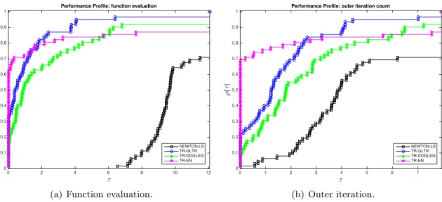
We consider first the TR algorithms. In Figure 1 the performance profiles show that TR-EN improves the efficiency of the TR algorithms on the tested problems. In fact, the outer iteration performance profiles (see Figure 1(b)) show that the use of the energy norm leads to a significant improvement on terms of the efficiency (for τ = 0, on 70% of the tested problems TR-EN performs the best, 23% for TR-GLTR, and around 10% for TR-DOGLEG). The use of the l

norm leads to a better robustness (i.e., TR-GLTR and TR-DOGLEG are solving a large percentage of the tested problem for large τ values). The same analysis applies in terms of function evaluation (see Figure 1(a)) where the efficiency of TR-GLTR and TR-DOGLEG is slightly improved compared to the out iterations performance profiles (but not as good as TR-EN). NEWTON-LS method is performing the worst on the tested problems, both in terms of efficiency and robustness.

For the ARC algorithms, see Figure 2, the performance profiles show that the use of the

energy norm (i.e., ARC-EN) improves the efficiency of the ARC algorithms over the tested prob-

lems. Unlike the TR performance profiles, NEWTON-LS is the most efficient method in terms of the

τ

0 2 4 6 8 10 12

ρ(τ)

0 0.1 0.2 0.3 0.4 0.5 0.6 0.7 0.8 0.9 1

Performance Profile: function evaluation

NEWTON-LS TR-GLTR TR-DOGLEG TR-EN

(a) Function evaluation.

τ

0 1 2 3 4 5 6 7

ρ(τ)

0 0.1 0.2 0.3 0.4 0.5 0.6 0.7 0.8 0.9 1

Performance Profile: outer iteration count

NEWTON-LS TR-GLTR TR-DOGLEG TR-EN

(b) Outer iteration.

Figure 1: TR performance profiles for the 62 optimization problems under consideration.

outer iteration number, see Figure 2(b). In fact, on over 50% of the tested problems NEWTON-LS performs the best, while ARC-EN solves 28% and ARC-GLTR around 20%. Regarding the function evaluation performance profile, see Figure 2(a), NEWTON-LS method looses its efficiency due to the backtracking strategy employed for each outer iteration. ARC-EN outperforms (by far) both solvers on terms of efficiency (in over 76% of the tested problems ARC-EN performs the best, and around 24% for ARC-GLTR). In terms of robustness, ARC-GLTR and ARC-EN exhibit similar performance. Again, as for TR algorithms, NEWTON-LS is performing the worst on the tested problems regarding the robustness.

τ

0 1 2 3 4 5 6 7 8

ρ(τ)

0 0.1 0.2 0.3 0.4 0.5 0.6 0.7 0.8 0.9 1

Performance Profile: function evaluation

NEWTON-LS ARC-GLRT ARC-EN

(a) Function evaluation.

τ

0 1 2 3 4 5 6 7 8

ρ(τ)

0 0.1 0.2 0.3 0.4 0.5 0.6 0.7 0.8 0.9 1

Performance Profile: outer iteration count

NEWTON-LS ARC-GLRT ARC-EN

(b) Outer iteration.

Figure 2: ARC performance profiles for the 62 optimization problems under consideration.

5.3 Test problems with many degrees of freedom

In this section we solve three large scale convex optimization problems from [13]. The first one is called MINSURF and consists of finding the surface with minimal area that lies above an obstacle with given boundary conditions. The second optimization problem, called IP, is an inverse problem from image processing. The third test case, called IGNISC, is an optimal-control problem related to a solide-ignition model. MINSURF and IGNISC are tested with n = 10000, for the IP optimization our tests are performed using n = 3969. The initial iterate for all the tested algorithms and problems is set to zero.

In our previous numerical experiments we solved exactly the subproblem (9). However, for large scale optimization problems finding the exact solution may be out of reach. In this section for TR-EN, ARC-EN and NEWTON-LS, such case is geared by mean of the truncated CG method.

The solvers TR-EN/ARC-EN and NEWTON-LS will be compared to TR-GLTR/ARC-GLRT. For the TR comparison, the TR-dogleg approach will be replaced by TR-ST which denotes a TR method that uses the Steihaug-Toint approach [7] to approximate the solution of TR subproblems. The TR-ST is the most commonly used in TR methods for approximating the solution of large scale TR sub-problems. The subproblem solvers GLTR and GLRT are tested using the default parameters (as in GALAHAD [12]). The NEWTON-LS and TR-ST subproblems are declared to be solved when the relative residual error is getting less than 10

.

For TR-EN/ARC-EN, we use a stopping criterion of the form (26). To quantify the sensibility of such termination condition (i.e., s-rule) two different values of κ

(1 and 10

are tested). Each iteration of the steps 1, 2 and 3 of TR-EN/ARC-EN (see Algorithm 2) formed an outer iteration.

Within each outer iteration, we must solve the minimization problem involving m

(s) at step 2 by means of the aforementioned truncated CG method. This procedure will be called the inner iteration minimization.

Figure 3 depicts the values of the objective function over outer iterations during the appli- cation of TR/ARC algorithms on the three large scale optimization problems. For all the tested algorithms the variation of the objective function value is more significant at the early stages of the optimization process. The TR-EN/ARC-EN algorithms outperform the other methods on the tested problems. In fact, for the three optimization problems, the use of the energy norm ensures a better decrease on the objective function value with a faster convergence speed. For the TR comparison, TR-ST and TR-EN (with κ

= 10

) give comparable performance in terms of outer iterations and converge faster than the other methods on the tested problems (i.e., in less than 10 outer iterations).

The TR-EN/ARC-EN algorithms are performing better using an accurate termination condi- tion, i.e., κ

= 10

. A high accuracy on the termination conditions can be computationally very demanding in terms of the inner iterations number. Table 2 outlines such a statement on the tested problems, it shows the variation of the number of inner iterations during the application of TR-EN/ARC-EN algorithms. As expected, for a large value of κ

, the number of inner iterations is by far less than the number required when using a tight termination condition. We note also that, for the tested problems, the choice of κ

is problem dependent. In fact, for MINSURF and IP problems the obtained results with the two different accuracies κ

= 1 and 10

are still very close, meaning that the choice of κ

does not affect significantly the number of outer iterations.

However, for IGNISC problem, the accuracy of the termination condition affects the speed of

convergence.