HAL Id: insu-03230914
https://hal-insu.archives-ouvertes.fr/insu-03230914
Submitted on 20 May 2021
HAL is a multi-disciplinary open access
archive for the deposit and dissemination of
sci-entific research documents, whether they are
pub-lished or not. The documents may come from
teaching and research institutions in France or
abroad, or from public or private research centers.
L’archive ouverte pluridisciplinaire HAL, est
destinée au dépôt et à la diffusion de documents
scientifiques de niveau recherche, publiés ou non,
émanant des établissements d’enseignement et de
recherche français ou étrangers, des laboratoires
publics ou privés.
Causes of the long-term variability of southwestern
South America precipitation in the IPSL-CM6A-LR
model
Julian Villamayor, Myriam Khodri, Ricardo Villalba, Valérie Daux
To cite this version:
Julian Villamayor, Myriam Khodri, Ricardo Villalba, Valérie Daux. Causes of the long-term
variabil-ity of southwestern South America precipitation in the IPSL-CM6A-LR model. Climate Dynamics,
Springer Verlag, 2021, �10.1007/s00382-021-05811-y�. �insu-03230914�
(will be inserted by the editor)
Causes of the long-term variability of southwestern
1
South America precipitation in the IPSL-CM6A-LR
2
model
3
Juli´an Villamayor · Myriam Khodri ·
4
Ricardo Villalba · Val´erie Daux
5
Received: date / Accepted: date
6
Abstract Southwestern South America (SWSA) has undergone frequent and
per-7
sistent droughts in recent decades with severe impacts on water resources, and
8
consequently, on socio-economic activities at a sub-continental scale. The local
9
drying trend in this region has been associated with the expansion of the
sub-10
tropical drylands over the last decades. It has been shown that SWSA
precipi-11
tation is linked to large-scale dynamics modulated by internal climate variability
12
and external forcing. This work aims at unravelling the causes of this long-term
13
trend toward dryness in the context of the emerging climate change relying on a
14
large set simulations of the state-of-the-art IPSL-CM6A-LR climate model from
15
the 6th phase of the Coupled Model Intercomparison Project. Our results
iden-16
tify the leading role of dynamical changes induced by external forcings, over the
17
local thermodynamical effects and teleconnections with internal global modes of
18
sea surface temperature. Our findings show that the simulated long-term changes
19
of SWSA precipitation are dominated by externally forced anomalous expansion
20
of the Southern Hemisphere Hadley Cell (HC) and a persistent positive Southern
21
Annular Mode (SAM) trend since the late 1970s. Long-term changes in the HC
ex-22
F. Author
LOCEAN-IPSL, Sorbonne Universit´e/CNRS/IRD/MNHN
4 place Jussieu 75005 Paris, France E-mail: julian.villamayor@locean.ipsl.fr
tent and the SAM show strong co-linearity. They are attributable to stratospheric
23
ozone depletion in austral spring-summer and increased atmospheric greenhouse
24
gases all year round. Future ssp585 and ssp126 scenarios project a dominant role
25
of anthropogenic forcings on the HC expansion and the subsequent SWSA
dry-26
ing, exceeding the threshold of extreme drought due to internal variability as soon
27
as the 2040s, and suggest that these effects will persist until the end of the 21st
28
century.
29
Keywords Subtropical Andes drying trend · Hadley Cell expansion · Decadal
30
variability · External forcing · CMIP6 · Detection and attribution · Future
31
scenarios
32
1 Introduction
33
The southwestern South America (SWSA) region encompasses the Andean Cordillera
34
and adjacent territories from the Pacific coast to the continental arid lowlands in
35
Argentina and south of the dry Altiplano. This region is characterized by a marked
36
precipitation gradient from < 100 mm in the north (25 - 28◦ S) to well over 2000
37
mm in the south (40 - 45◦S). Precipitation primarily occurs during austral winter
38
(June-August, JJA) associated with passing fronts embedded in the mid-latitude
39
Westerly flow and enhanced by the orographic effect of the Andes Mountains
40
(Montecinos and Aceituno, 2003; Garreaud et al., 2013; Viale et al., 2019).
Lati-41
tudinal variations in the southeastern Pacific anticyclone and the subtropical jet
42
stream modulate the seasonality of these fronts, which commonly form at the
43
poleward limit of the Southern Hemisphere (SH) Hadley Cell (HC) (Montecinos
44
and Aceituno, 2003; Barrett and Hameed, 2017). Closely linked to large-scale
at-45
mospheric circulation, SWSA precipitation supports the many glaciers and lakes
46
in the Andes and contributes to the flow of major streams and rivers along the
47
Cordillera. Indeed, most rivers originate in the upper Andes, where precipitation
48
is comparatively higher than in adjacent territories (Masiokas et al., 2019). With
49
some regional differences, SWSA has undergone a striking drying trend since the
1980s (e.g., Garreaud et al., 2013, 2017, 2020; Boisier et al., 2016, 2018), with
51
marked glacier retreats and lake-area reductions without precedent over the last
52
millennium (Garreaud et al., 2017; Pab´on-Caicedo et al., 2020). A robust drying
53
trend of around -28 mm per decade during the austral winter rainy season has been
54
found in the southern part of SWSA (Boisier et al., 2018). In the northern drier
55
regions, the larger amplitude of the high-frequency variability in austral summer
56
(December-February, DJF) and fall (March-May, MAM) complicates the detection
57
of consistent trends in precipitation. However, a reduction in river streamflows
sug-58
gests that a drying tendency is also taking place in spring (September-October,
59
SON) and summer in the north sector of SWSA (Boisier et al., 2018). Although
60
they display lower drought than observed, model simulations for the historical
pe-61
riod of the 5thphase of the Coupled Model Intercomparison Project (CMIP5) can
62
capture such drying tendency in response to external anthropogenic forcings (Vera
63
and D´ıaz, 2015; Boisier et al., 2018). Due to the important socio-economic and
eco-64
logical impacts of changes in water resources in SWSA (CR2, 2015; Norero and
65
Bonilla, 1999; Rosegrant et al., 2000; Meza et al., 2012), it is critical to investigate
66
further and quantify the potential impacts of climate change in this region.
67
Low-frequency rainfall changes in SWSA are also associated with internal
cli-68
mate variability. Indeed, during austral winter and spring, SWSA annual moisture
69
conditions are tightly linked to the southeastern Pacific sea surface temperature
70
(SST) variability (Rutllant and Fuenzalida, 1991; Garreaud et al., 2009; Quintana
71
and Aceituno, 2012; Boisier et al., 2016) related to the El Ni˜no Southern
Oscil-72
lation (ENSO), the leading mode of interannual climate variability in the Pacific
73
Ocean (e.g., McPhaden et al., 2006). Long-term ENSO fluctuations imprint a
pan-74
Pacific pattern of coherent SST decadal variability (Newman et al., 2016) through
75
atmospheric teleconnections (e.g., Alexander et al., 2002). This pattern is known
76
as the Interdecadal Pacific Oscillation (IPO) and is the leading mode of
inter-77
nal, decadal to multidecadal variability in the Pacific Ocean (Folland et al., 1999;
78
Meehl and Hu, 2006). It is also typically referred to as its manifestation in the
wintertime North Pacific SST, the so-called Pacific Decadal Oscillation (Mantua
80
et al., 1997). During the positive (negative) phase, the IPO is characterized by
81
an ENSO-like pattern of warm (cold) SST anomalies across the tropical Pacific,
82
which extends in the subtropics over the eastern boundaries of the Pacific Ocean
83
(Trenberth and Hurrell, 1994; Meehl et al., 2009). The IPO has experienced a
84
trend from a positive (i.e., El Ni˜no-like) to a negative (La Ni˜na-like) phase over
85
the 1980-2014 period associated with an anomalous southward shift and spin-up of
86
the southeastern Pacific anticyclone (Jebri et al., 2020) and of the mid-latitudinal
87
storm-tracks over SWSA during the rainy season (Quintana and Aceituno, 2012;
88
Boisier et al., 2016, 2018).Thus, the concurrent IPO shift from positive to
nega-89
tive phase might have contributed to the current prevailing SWSA dry conditions
90
(Masiokas et al., 2010; Quintana and Aceituno, 2012; Boisier et al., 2016).
How-91
ever, during DJF and MAM seasons, rainfall interannual-to-decadal fluctuations
92
are also significantly influenced by the dominant mode of atmospheric circulation
93
variability in the mid-latitudes of the SH, the Southern Annual Mode (SAM),
94
also known as the Antarctic Oscillation (Gong and Wang, 1999; Thompson and
95
Wallace, 2000; Thompson et al., 2000). During SAM positive phases, a zonally
96
symmetric atmospheric pressure gradient is observed with negative and positive
97
anomalies over Antarctica and the mid-latitudes, respectively, favoring an
anoma-98
lous poleward shift of the circumpolar westerlies and more constrained zonal flow
99
in mid-latitudes (Thompson and Wallace, 2000; Thompson et al., 2000), resulting
100
in less frontal rainfall in SWSA (Garreaud et al., 2009). These symmetric features
101
and the impact on SWSA precipitation are reversed during the negative SAM
102
phase.
103
The SWSA drying trends over recent decades could also result from external
104
forcings. For instance, an intensification of the global hydrological cycle is projected
105
under global warming due to a more extensive water vapour loading of the
atmo-106
sphere, resulting in enhanced E-P (evaporation minus precipitation) in evaporative
107
regions, and reduced E-P in precipitative regions according to the ”wet-get-wetter,
dry-get-drier” paradigm (Helpd and Soden, 2006; Seager et al., 2010). Several
ob-109
servational datasets, CMIP5 models and reanalyses also suggest an essential role
110
of externally forced large-scale dynamical changes. Observed southward shifts of
111
the subtropical drying regions and mid-latitudes baroclinic eddies during late
aus-112
tral spring and summer have been associated with the SAM positive trend and
113
the expansion of the HC in recent decades (e.g., Gillett and Thompson, 2003;
Pre-114
vidi and Liepert, 2007; Quintana and Aceituno, 2012; Boisier et al., 2018). The
115
HC expansion and SAM positive trends have both been attributed to increasing
116
atmospheric greenhouse gases (GHGs) concentration and stratospheric ozone
de-117
pletion (e.g., Polvani et al., 2011; Kim et al., 2017; Jebri et al., 2020). However, the
118
tendency toward more La Ni˜na events in relation to the recent IPO trend may also
119
contribute to the HC poleward shift (Nguyen et al., 2013; Allen and Kovilakam,
120
2017) and to more frequent positive SAM phases (Carvalho et al., 2005; Fogt et al.,
121
2012). The counteracting effect of the recent ozone recovery (Eyring et al., 2010)
122
and the intensification of GHGs effect (Andreae et al., 2005) is a source of
uncer-123
tainty for the understanding of the future state of these modes (Fogt and Marshall,
124
2020).
125
To our knowledge, previous studies have not explicitly examined (i) the
re-126
spective contribution of anthropogenic forcing and internal climate variability on
127
the decadal-to-longer term variance of SWSA rainfall throughout the last century
128
and a half and (ii) the specific role of direct thermodynamical and dynamical
129
changes in SWSA related to the HC expansion and SAM trend. These are two
130
major points that are addressed in this study along with (iii) the attribution of
131
the modulation of SWSA precipitation to specific sources of external forcing over
132
the last decades (iv) and its projected changes for the 21st century. Here, we
as-133
sess the SWSA hydroclimate changes over the last century using observations,
134
reanalyses and sets of 20 to 32 member-ensemble simulations conducted with the
135
stand-alone LMDz6A-LR atmospheric component (Hourdin et al., 2020) and the
136
IPSL-CM6A-LR coupled model (Boucher et al., 2020) as part of the 6th phase
of the CMIP exercise (CMIP6; Eyring et al., 2016). The paper is organized as
138
follows: in the next two sections, the data and methods used are introduced, the
139
results obtained are presented in section 4 and discussed in section 5. A summary
140
and the main conclusions are provided in section 6.
141
2 Data
142
2.1 The atmospheric and coupled model
143
We used the CMIP6 version of the Institut Pierre- Simon Laplace (IPSL)
stand-144
alone atmosphere model, called LMDz6A-LR (Hourdin et al., 2020) and the
cou-145
pled atmosphere-ocean general circulation model (GCM), called IPSL-CM6A-LR
146
(Boucher et al., 2020). LMDz6A-LR is coupled to the ORCHIDEE (d’Orgeval
147
et al., 2008) land surface component, version 2.0. In IPSL-CM6A-LR, the
LMDz6A-148
LR is coupled to the oceanic component Nucleus for European Models of the
149
Ocean (NEMO), version 3.6, which includes other models to represent sea-ice
150
interactions (NEMO-LIM3; Rousset et al., 2015) and biogeochemistry processes
151
(NEMO-PISCES; Aumont et al., 2015). LR stands for low resolution, as the
at-152
mospheric grid resolution is 1.25◦ in latitude, 2.5◦ in longitude and 79 vertical
153
levels (Hourdin et al., 2020). Compared to the 5A-LR model version and other
154
CMIP5-class models, IPSL-CM6A-LR was significantly improved in terms of the
155
climatology, e.g., by reducing overall SST biases and improving the latitudinal
156
position of subtropical jets in the SH (Boucher et al., 2020). The IPSL-CM6A-LR
157
is also more sensitive to CO2 forcing increase (Boucher et al., 2020) and
repre-158
sents a more robust global temperature response than the previous CMIP5 version
159
consistently with current state-of-the-art CMIP6 models (Zelinka et al., 2020).
160
2.2 Experimental protocol
161
This study is based on a set of climate simulations generated as part of CMIP6
162
(Table 1). We relied on the pre-industrial control (piControl) coupled run with
the external radiative forcing fixed to pre-industrial values for a measure of the
164
internal climate variability generated by the IPSL-CM6A-LR model.
165
We also used the 32-member ensemble of simulations for the historical period
166
(1850-2014), which is branched on random initial conditions from the piControl
167
run to ensure that ensemble members are largely uncorrelated during the
simu-168
lation. All 32 members of this ensemble (referred to as the historical ensemble)
169
use the historical natural and anthropogenic forcings following CMIP6 protocol
170
(Eyring et al., 2016). They include concentrations of GHGs from 1850 to 2014
171
provided by (Meinshausen et al., 2017) while the standard CMIP6 tropospheric
172
and stratospheric ozone concentration were obtained from the Chemistry-Climate
173
Model Initiative (Checa-Garcia et al., 2018). Tropospheric aerosols, from
natu-174
ral and anthropogenic sources (Hoesly et al., 2018; van Marle et al., 2017) are
175
also included along with historical stratospheric natural forcings, corresponding
176
to spectral solar irradiance-stratospheric ozone cycles (Matthes et al., 2017) and
177
the main volcanic eruptions prescribed with the aerosol optical depth (Thomason
178
et al., 2018).
179
Detection and attribution 10-member ensembles (Gillett et al., 2016) are also
180
utilized to understand the role of the different external forcing components in the
181
context of climate change. These experiments are equivalent to the historical ones
182
but include each forcing individually namely either GHGs (hist-GHG),
strato-183
spheric ozone depletion (hist-stratO3), aerosols (hist-aer) and natural (hist-nat)
184
while maintaining other forcing at their 1850 level.
185
Two 6-member ensembles for the 21stcentury (2015-2100) future projections
186
scenarios branched on randomly selected historical members at the year 2014 are
187
also analyzed (O’Neill et al., 2016): the ssp585 equivalent to ∼8.5 W m-2
in-188
creased radiative forcing in the year 2100 due to GHG emissions (the highest
189
future pathway across all CMIP6 scenarios) and the ssp126 mitigation scenario,
190
which assumes the lowest of plausible radiative forcing effects (2.6 W m-2) in 2100
191
assuming substantial mitigation against global warming.
Finally, we also use AMIP historical (amip-hist) simulations, which use the
193
same external forcings since 1870 as the historical experiment but with imposed
ob-194
served monthly SST on the LMDz6A-LR atmospheric component. Further details
195
about external forcings implementation strategies in the experiments mentioned
196
above are given in Lurton et al. (2020).
197
2.3 Observational data
198
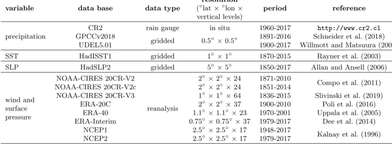
In addition to model outputs, different observational products are used: in situ
199
and gridded observations data sets and reanalyses (Table 2). We analyze in situ
200
monthly precipitation data from 1960 to 2017 from rain gauges in 129 stations
201
located along the Andes, between 70◦ - 73◦ W and 20.5◦ - 46.5◦ S provided
202
by the Chilean Center for Climate and Resilience Research, Climate Explorer
203
(http://explorador.cr2.cl) (Fig. 1). Note that the station coverage is relatively
204
sparse outside the 27◦ - 43◦ S region in SWSA. We also rely on gridded products
205
of monthly precipitation provided by the Global Precipitation Climatology Centre
206
(version 2018; GPCCv2018) and the University of Delaware Air Temperature and
207
Precipitation (version 5.01; UDEL5.01), each of which using different
interpola-208
tion methods. Note in Fig. 1 that the data coverage of the observations used for
209
the reconstruction of these gridded products is consistent with that of the in situ
210
observations, which are quite sparse outside SWSA in southern South America.
211
We use the Hadley Centre Sea Ice and Sea Surface Temperature version 1
212
(HadISST) gridded reconstruction of SST observations, which are used as
bound-213
ary conditions in the LMDz6A-LR model amip-hist CMIP6 simulations. To study
214
the atmospheric dynamics, we also analyze the meridional wind and the
sur-215
face pressure variables from several reanalyses: the NOAA-CIRES 20th Century
216
Reanalysis versions 2 (20CRv2), 2c (20CRv2c) and 3 (20CRv3), the ERA-20C,
217
ERA40 and ERA-Interim reanalyses of the European Centre for Medium-Range
218
Weather Forecasts and the National Center for Environmental Prediction (NCEP)
and the National Center for Atmospheric Research (NCAR) reanalysis version 1
220
(NCEP1) and 2 (NCEP2).
221
3 Methods
222
3.1 Trend analyses and statistical testing
223
All anomalies are calculated by removing the monthly mean seasonal cycle of the
224
entire covered period (Table 1) from the time series before calculating seasonal
av-225
erages (MAM, JJA, SON and DJF). To focus only on the variability from decadal,
226
interdecadal or longer time scales, time series are low-pass filtered (LPF) using a
227
Butterworth filter with a cut-off period of 8, 13 or 40 years, respectively
(But-228
terworth, 1930). The linear trend for each month over 1979-2014 is obtained by
229
applying least squares on unfiltered yearly time series of monthly mean
precipi-230
tation and represented in terms relative to the climatological mean (% decade-1).
231
In this case, trend values are statistically tested with a Student t-test with the
232
number of degrees of freedom corresponding to the total number of years minus
233
one. To evaluate the ensemble-mean trend representativeness, we also indicate the
234
regions where at least 80% of the members display trends of the same sign than
235
the ensemble mean. The consistency between the anomalies of the climate
param-236
eters and the modes of variability was estimated using the regression coefficient
237
(α) between these variables. When the time series are spatially distributed the
re-238
sulting regression coefficients are presented as regression patterns. In this case, the
239
ensemble-mean regression coefficients are statistically tested using a random-phase
240
test, based on Ebisuzaki (1997), adapted to the regression (details in Villamayor
241
et al. (2018)). In turn, the level of uncertainty among individual members is
indi-242
cated by showing the grid points, where at least 80% of them display a regression
243
coefficient of the same sign as the ensemble mean. When considering regionally
244
averaged time series for the ensemble mean, the uncertainty of the resulting
gression coefficient is quantified by representing the range of values obtained with
246
all members individually.
247
3.2 Climate indices
248
We consider five main sets of climate indices that are introduced below. Note that
249
for ensemble simulations, the ensemble-mean index refers to the indices calculated
250
from outputs previously averaged across all members. The 95% confidence interval
251
among individual members, according to a Student t-test, is shown to quantify the
252
uncertainty of the ensemble-mean indices .
253
3.2.1 SWSA precipitation indices
254
Empirical Orthogonal Function analysis of the 8-year LPF rainfall anomalies in
255
southern South America (25◦ - 58◦ S, 65◦ - 80◦ W) is performed to isolate the
256
leading mode of variability at decadal-to-longer time scales. The first Principal
257
Component (PC1) for each season is standardized to get a measure of the
vari-258
ance. Regions with the highest variance are then used to build regional indices by
259
averaging values over: 34◦ - 49◦ S, 71◦ - 77◦ W in MAM; 28◦ - 40◦ S, 70◦ - 76◦
260
W in JJA; 30◦ - 43◦S, 70◦- 77◦ W in SON and 39◦- 50◦ S, 72◦ - 78◦W in DJF.
261
3.2.2 Global Warming and IPO sea surface temperature indices
262
A global warming index (GW) is calculated by spatially averaging 40-year LPF
263
annual-mean SST anomalies (SSTAs) over 45◦S - 60◦N. Residual SSTAs are then
264
derived by regressing out the GW SSTAs pattern. To analyze the IPO influence on
265
SWSA rainfall, an IPO index is computed using the residual SSTA following the
266
tripole approach of Henley et al. (2015), defined as the central equatorial Pacific
267
SST (10◦ S - 10◦ N, 170◦ E - 90◦ W) minus the average of northwest (25◦ - 45◦
268
N, 140◦ E - 145◦ W) and southwest (15◦ - 50◦ S, 150◦ E - 160◦ W) Pacific SST.
269
The resulting IPO index is then LPF with a 13-year cut-off period.
3.2.3 Southern Annular Mode and Hadley Cell extent indices
271
Seasonal SAM indices are computed for each season as the standardized PC1 of
272
the 8-year LPF sea level pressure (SLP) anomalies in the SH, south of 20◦ S. In
273
order to describe the variability of the latitudinal position of the poleward edge of
274
the HC in the SH, we define an index of the HC extent (HCE) for each season as
275
the linearly interpolated latitude for which the 500-hPa meridional streamfunction
276
(ψ500) is equal to zero between 20◦ and 40◦ S.
277
3.3 Decomposition of SWSA precipitation variance
278
A decomposition of the variance of SWSA precipitation into the components
ex-279
plained by the IPO and the GW SST indices is performed based on a multilinear
280
regression analysis (Mohino et al., 2016). According to this, the total variance of
281
SWSA precipitation (var[P R]) can be expressed in terms of the regression
coeffi-282
cients from the multilinear fitting that correspond to each index (αIPO and αGW,
283
respectively) and a residual (var[ε]) as follows:
284
var[P R] = αIP O2+ αGW2+ var[ε] (1)
The residual term stands for the variance of the residual of the multilinear fitting,
285
namely the variance that cannot be explained by the IPO and the GW indices.
286
These three components are expressed as percentage of the total variance of SWSA
287
precipitation.
288
3.4 Total moisture budget decomposition
289
A decomposition of the change in the net moisture budget, expressed as
precipi-290
tation minus evaporation (P-E), into purely thermodynamic and dynamic
compo-291
nents is performed in this work. According to the moisture budget equation, P-E
292
equals the divergence of the moisture flux (Brubaker et al., 1993). The moisture
flux is the mass-weighted and vertical integral of the product between the specific
294
humidity (q) and the horizontal winds (u). Therefore, a change in P-E (δ(P − E))
295
implies changes in q (i.e., thermodynamic changes (δT H) and u (i.e., dynamic
296
changes (δDC). Considering such a change as an anomaly with respect to a
ref-297
erence period (denoted with subscript r), the thermodynamic and the dynamic
298
components can be separated using the following approach (Seager et al., 2010):
299
δ(P − E) = δT H + δDC + RES (2)
Following Ting et al. (2018), we define δT H and δDC as follows:
300 δT H ≈ − 1 gρw · ∇ ps Z 0 ur· δq dp (3) 301 δDC ≈ − 1 gρw · ∇ ps Z 0 δur· q dp (4)
where g is the gravitational acceleration, ρw the density of water, p pressure levels
302
and psthe surface pressure.
303
The residual component (RES) mostly accounts for the moisture convergence
304
changes due to transient eddies, but also includes nonlinear terms that are typically
305
neglected in the approach of δT H and δDC (Seager et al., 2010; Ting et al., 2018).
306
3.5 Probability Density Functions of precipitation linear trend
307
To further evaluate the role of the IPO phase shift (such as during the 1979-2014
308
period) on SWSA precipitation trends in our model as compared to observations,
309
we performed Probability Density Functions (PDFs) of the linear trend of SWSA
310
precipitation for 36-year periods separately for ensemble members with a positive
311
or negative IPO trend that is significant at the 5% level during the period
(re-312
sulting in 25 members of each category). The two resulting PDFs are statistically
313
compared by testing the null hypothesis that both present independent normal
distributions with equal means and equal but unknown variances at the 20%
sig-315
nificance level, according to a t-test. A t-test is also used to evaluate whether mean
316
trend values are significantly different from zero.
317
4 Results
318
4.1 Model validation
319
In this section, we present a comparison of the amip-hist and historical simulations
320
with observational products to evaluate the ability of, respectively, the atmospheric
321
component and the coupled model to simulate main aspects of precipitation in
322
SWSA, such as climatology and tendency. We also check simulated IPO phase
323
shifts and the emerging HC expansion, which are addressed in relation to the
324
recent drying trend in SWSA.
325
4.1.1 SWSA precipitation
326
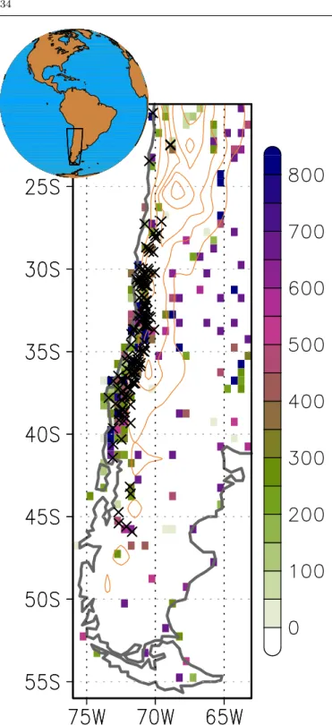
The SWSA region rainfall annual cycle over the period common to observations
327
and simulations (1960-2014) is represented in Fig. 2 (left panel). Considering the
328
spatial coverage of observations in SWSA (Fig. 1), the model validation is
re-329
stricted to a latitudinal band between 20◦ - 47◦ S. This band is roughly 5◦
longi-330
tude width (i.e., two grid points in the model) and centered in 73.75◦W. Most of
331
the rain gauge stations are located in the west Chilean territories adjacent to the
332
Andes where precipitation is enhanced by the orographic blocking effect on the
333
westerly atmospheric flow (Falvey and Garreaud, 2007; Smith and Evans, 2007;
334
Viale et al., 2019). The rain gauge observed annual cycle shows a latitudinal
migra-335
tion of rainfall sustaining marked dry and wet seasons in austral summer (DJF)
336
and winter (JJA), respectively (Fig. 2a). The onset of the rainy season occurs
337
gradually during fall (MAM), with maximum rainfalls registered around 37◦ S in
338
June. This regional maximum is not well captured by the gridded observations,
339
most likely because of interpolation procedures applied to rain gauge data (Figs.
2c and 2e). The rainy season demise occurs in spring (SON), before minimum
341
values are reached in summer.
342
The amip-hist and historical simulations reproduce the observed mean annual
343
cycle, with the onset in MAM, the rainy season in JJA with a maximum in June
344
around 37◦ S, the demise in SON and the dry season in DJF (Figs. 2g and 2i).
345
The model seems to overestimate climatological values north of 35◦ S and south
346
of 40◦S. This discrepancy may instead be attributable to the lack of observations
347
at these latitudes. There is also a high level of uncertainties in observations
re-348
garding the climatological amount. Annual rainfalls reach around 1460 mm in rain
349
gauge observations where it is most rainy between 35◦S and 40◦S, while gridded
350
products values are about two thirds of this amount (i.e., 910 mm in GPCCv2018
351
and 890 mm in UDEL5.01). Model ensemble-means for amip-hist and historical
352
simulations amount 1670 and 1450 mm respectively, with an ensemble standard
353
deviation of around 25 mm in both cases, which is close to in situ observations.
354
However, historical simulations generally give smaller values than amip-hist,
espe-355
cially during the rainy season. This difference is independent of the size of both
356
ensembles (not shown) and most likely related to the influence of the observed
357
SSTs in amip-hist runs.
358
The annual cycle of the linear trend relative to the climatological mean over
359
the last 36 years (1979-2014) is represented in Fig. 2 (right panel). A significant
360
drying around 33◦ - 40◦S in April-May and around 29◦- 36◦S in July is observed
361
consistently in all observations datasets (Figs. 2b,d,f). These drying trends indicate
362
a delay in the onset of the rainy season and less rainfall during the rainy season.
363
Although weak and not significant, negative trend values in September, together
364
with the features described before, suggest that, in general, there is a tendency
365
towards shorter and less effective rainy season in SWSA over the last decades.
366
The H¨ovmoller diagrams from gridded observations show positive trend during
367
late spring and summer south of 40◦ S, suggesting that the southernmost part of
SWSA has become wetter (Figs. 2d and 2f). However, this result is poorly reliable
369
due to the lack of observations in this part of the Andes (Fig. 1).
370
Both amip-hist and historical simulations indicate a widespread drying
rela-371
tive to the simulated climatology along the year, with a maximum from around
372
∼40◦ S in DJFM to ∼27◦ S in MJJAS (Figs. 2h and 2j), suggesting a
shorten-373
ing and weakening of the rainy season. The drying trend is in general stronger
374
in amip-hist simulations than in historical runs (independently of the ensemble
375
size, not shown). All amip-hist members include the same observed SST, while
376
in historical simulation, SST variability is largely uncorrelated among ensemble
377
members. Averaging the historical ensemble allows therefore damping the
influ-378
ence of SST on the simulated rainfall trends with respect to the role of external
379
forcing. Differences with amip-hist on the other hand, emphasize the contribution
380
of observed SST variability. The drying trend during the onset and demise of the
381
rainy season is more intense and significant in the amip-hist ensemble mean than
382
in the historical one. This suggests a dominant role of observed SST variability
383
(such as the shift toward a negative IPO) in the rainy season shortening during
384
1979-2014, probably amplified by external forcing influence.
385
To summarize, despite the constraints of comparing local observations with
386
gridded data from GCMs due to the complex orography of the region, the model
387
can reproduce the main observed rainfall climatological features and recent trends.
388
Differences between the amip-hist and the historical coupled simulations suggest
389
a combination of internal and external factors in driving the SWSA drying trend.
390
Previous generation CMIP5 models show an overall underestimation of the SWSA
391
precipitation response to external forcing (Vera and D´ıaz, 2015; Boisier et al.,
392
2018) that is coherent with the IPSL-CM6A-LR simulations. On the other hand,
393
a preliminary CMIP6 multi-model study places the IPSL-CM6A-LR among the
394
GCMs that best represent the atmospheric changes over southeast Pacific that
395
modulate SWSA rainfall during the last century (Rivera and Arnould, 2020), which
supports the use of this model to study the long-term precipitation variability in
397
this region.
398
4.1.2 IPO phase shifts
399
We also evaluate the model ability to simulate IPO phase shifts comparable to the
400
observed shift over the 1979-2014 period addressed by Boisier et al. (2016) in terms
401
of the amplitude of the associated SST anomalies. To this aim, Fig. 3 represents
402
IPO indices from observational data (HadISST1) over 1870-2014 and from the
403
piControl run over a representative period of equal length, as well as the linear
404
trend values obtained along both IPO indices in centered running windows of 15-40
405
years long. The trend graphics show blue and red colored plumes, corresponding
406
to negative and positive trend values, respectively. The plumes resulting from the
407
piControl IPO index are, in general, narrower than those from observations. This
408
reveals that the model underestimates the observed persistence of the IPO phases.
409
However, the model succeeds in simulating 36-year IPO phase shifts of up to -0.2
410
◦C per decade comparable to the one observed over 1979-2014.
411
4.1.3 Hadley Cell expansion
412
To evaluate the model’s ability to reproduce the HC expansion in recent decades,
413
we compare the linear trend of the seasonal HCE indices calculated with eight
414
different reanalyses and the amip-hist and historical simulations for their common
415
23-year period (1979-2001) and for a 40-year period (1971-2010), common to the
416
simulations and five reanalyses (Fig. 4). The trend values obtained over the short
417
period show large dispersion between the different members of the amip-hist and
418
historical simulations, compared with those of the longer period. This shows the
419
dependence of the tendency of the HCE index on short-term stochastic internal
420
variability. In the longer term, the trend is more robust across model members
421
suggesting an influence of external forcings. Comparing across seasons, the
simu-422
lated HCE trend is better constrained among members in JJA and most uncertain
in DJF, when the HC is most variant and presents wider expansion. Regarding
424
observations, the trend values obtained from reanalyses show large spread as well.
425
Despite the large uncertainty, when the 40-year long period is considered, there is
426
solid agreement among reanalyses regarding the Southern HC expansion towards
427
the pole in recent decades (Grise et al., 2019).
428
The model simulates trends that are within the range of those in the
reanal-429
yses. The trend of the simulated HCE in the ensemble mean is negative in all
430
seasons and in both amip-hist and historical simulations, being widest in DJF. In
431
MAM, the poleward expansion of the HCE is the weakest and close to zero when
432
simulated by the historical simulation, while the amip-hist simulation shows a
433
broader expansion. In contrast, during the other seasons, the simulated
ensemble-434
mean expansion is similar in both simulations, being wider in the historical over
435
the 40-year-period. These results suggest that the external forcing mostly induces
436
the HC poleward expansion in JJA, SON and particularly in DJF, but in MAM
437
this effect is weak and, presumably, the influence of SST internal variability is also
438
relevant.
439
4.2 Relative roles of forced versus internal variability on SWSA precipitation
440
decadal variability and trend
441
In this subsection, we focus on the amip-hist ensemble to unravel the contribution
442
of observed SST to SWSA precipitation low-frequency variability. The first PCs
443
of the 8-year LPF seasonal precipitation anomalies account for much of the total
444
decadal-scale rainfall variability in southern South America (25◦- 58◦ S; 65◦- 80◦
445
W). The explained total variance of the PC1 is 59.1% in MAM, 75.7% in JJA,
446
67.0% in SON and 69.9% in DJF. These indices together with their respective
447
regression patterns show that most of the precipitation variability in southern
448
South America is concentrated in a dipole of opposite anomalies between the
449
middle (25◦- 45◦S) and high (> 50◦ S) latitudes in SWSA (Fig. 5). The seasonal
450
patterns in DJF and MAM also present significant anomalies in subtropical South
America east of the Andes showing an opposite sign to those recorded in middle
452
SWSA latitudes.
453
These regression patterns allow identifying where the most substantial
low-454
frequency variability occurs in the amip-hist simulations (boxed areas in Fig. 5).
455
These regions vary depending on the season, showing a north-to-south shift from
456
winter (JJA) to summer (DJF), respectively, and are co-located with the centers
457
of maximum rainfall linear trends (gray contours in Fig. 5). These regions with
458
the most substantial negative rainfall anomalies are associated with PC1s positive
459
long-term trend (Fig. 5, left panels), which accounts for nearly the total tendency
460
of the area-averaged precipitation anomalies for each season (Table 3). From 1970
461
to 2014 a deficit of 6.2 mm per decade and around 15.2 mm per decade is simulated
462
for the rainy (JJA) and dry summer (DJF) seasons respectively.
463
Previous studies have shown evidence for the influence of SST internal
vari-464
ability and external forcings on SWSA rainfall recent changes (e.g., Boisier et al.,
465
2016, 2018). In line with these previous works and to identify potential connections
466
between simulated low-frequency variations of SWSA precipitation and observed
467
internal modes of climate variability, we regress PC1s on anomalies of SST, SLP
468
and wind (Fig. 6) before and after removing the long-term trend signal in PC1s
469
with a 3rd-degree polynomial fit (dotted lines in Fig. 5). Such detrending will allow
470
emphasizing typical SST and teleconnection patterns related to internal variability
471
modes.
472
Without detrending, SST regression patterns show warm anomalies almost
473
globally distributed except in the tropical Pacific where an IPO-like relative
cool-474
ing dominates all year round (left panel in Fig. 6). The warm pattern is most
475
widespread in DJF, with strong anomalies over western Pacific, the Indian and
476
Atlantic Oceans, especially in the southern basin, and weakest in JJA. In turn,
477
the tropical Pacific cooling is more intense in SON and JJA and almost negligible
478
in DJF and MAM. This global SST pattern is reminiscent of an IPO negative
479
phase combined with the global warming signal induced by external forcing. In
DJF and MAM surface winds and SLP anomalies show a poleward shift of the
481
westerlies and a SLP maximum slightly south of 30◦ S associated with the SWSA
482
drying. This suggests a link with the strengthening of the SAM with a weaker
483
influence of the negative IPO pattern on the SWSA drying in austral summer and
484
fall, in agreement with Boisier et al. (2018).
485
Regression patterns obtained with the detrended PC1s highlight a sea-level
486
pressure high and significant anomalous easterlies in Southeastern Pacific in JJA
487
and SON, suggesting an atmospheric teleconnection with a negative IPO-like SSTA
488
pattern most prominent in austral winter and spring (right panel in Fig. 6).
Ex-489
tratropical SLP anomalies are less zonally symmetric than with the non-detrended
490
PC1s with an anomalous jet of westerlies passing through SWSA south of around
491
45◦S, which is coherent with the anomalous SLP gradient. Therefore, this pattern
492
may suggest that, in response to a negative IPO, there is a poleward shift of the
493
storm-tracks embedded in the zonal flow (Garreaud et al., 2013), resulting in less
494
intrusion of humid air masses over middle latitudes in SWSA. Comparison of
re-495
gression patterns before and after PC1s detrending indicates therefore that
precip-496
itation trends in winter (JJA) and spring (SON) are largely influenced by internal
497
IPO related SST variability (Boisier et al., 2016). On the other hand, high-latitude
498
atmospheric circulation associated with the SST warming signal dominates SWSA
499
rainfall trends especially in summer (DJF) and fall (MAM) (e.g., Boisier et al.,
500
2018).
501
To further evaluate the respective roles of the global warming and internal SST
502
variability on SWSA precipitation, a multilinear regression analysis over
1870-503
2014 is performed using as predictands the simulated seasonal indices of SWSA
504
precipitation (i.e., area-weighted mean over boxed areas in Fig. 5) and the IPO
505
and GW observed SST indices as predictors (Fig. 7). The results show that the
506
IPO barely explains 19% and 15% of the precipitation low-frequency total variance
507
in JJA and SON, respectively, and that its contribution is almost null in MAM
508
and DJF (Fig. 7). The GW index explains a larger proportion of rainfall variance
in all the seasons except in JJA. The external forcing influence is exceptionally
510
remarkable in DJF, where the GW dominates the precipitation variance above the
511
IPO, which shows very little impact. However, the explained variance by the GW
512
index only represents the indirect external forcing influence on SWSA rainfalls
513
through induced SST anomalies. It does not account for the externally forced
514
changes in atmospheric dynamics and direct thermodynamic effects in SWSA.
515
The fact that the residual component is considerably large in all seasons suggests
516
that SST changes are not a significant driver of the SWSA precipitation variability
517
at decadal-to-longer time scales.
518
A possible explanation for the low response of the simulated SWSA
precipita-519
tion to the IPO could be due to the unrealistically weak atmospheric teleconnection
520
simulated by the model. However, the SLP anomalies regressively associated with
521
the IPO in JJA over southeastern Pacific (blue box in Fig. 6b) in HadSLP2
ob-522
servations (0.24 hPa per standard deviation) lies within one standard deviation
523
of the ensemble-mean values of the amip-hist and historical simulations
(respec-524
tively, 0.32 ± 0.14 and 0.34 ± 0.15 hPa per standard deviation). Hence, we cannot
525
attribute the relatively weak influence of the internal SST decadal variability on
526
simulated rainfall to insufficient sensitivity of the atmospheric component of the
527
model to SST anomalies.
528
The SWSA precipitation response to the IPO simulated in amip-hist,
histori-529
cal and piControl simulations (see Table 1) are shown in the bottom panel of Fig.
530
7. MAM and DJF rainfall responses are positive in the amip-hist and historical
531
ensembles, but weak and not emerging from the internal variability as represented
532
by the piControl simulation. In turn, this positive signal is significant in amip-hist
533
in JJA and SON, the strongest being in JJA. In the historical simulations, the
534
response to the IPO is also positive and strongest in JJA but not significant as
535
in all seasons, consistently with the unforced piControl run. These observation
536
suggest that the difference in the SWSA response to IPO between forced and
un-537
forced coupled model simulations is not significant. Therefore, according to these
results, it can be inferred that the IPO can impact on the simulated SWSA
pre-539
cipitation. Still, its influence is weak as compared to external forcing and only
540
robustly reproducible with the SST-forced amip-hist simulations in JJA and, to a
541
lesser extent, in SON. Next, we examine the relative influences of dynamical and
542
thermodynamical external forcings on the low-frequency variability and trend of
543
SWSA rainfalls.
544
4.3 Role of dynamical vs. thermodynamical changes in SWSA
545
In the previous subsection, anomalous poleward shift of the zonal circulation in
546
high-latitudes in the SH is attributed to external forcings. This suggests that
ex-547
ternal forcings act on SWSA precipitation through dynamical changes. However, it
548
has been shown that long-term dynamical changes cannot account for all the
exter-549
nally forced trend in subtropical precipitation with direct thermodynamic effects
550
playing an important role (Schmidt and Grise, 2017). Therefore, the question arises
551
as to whether the forced component of precipitation in SWSA is mostly induced
552
by dynamic or thermodynamic processes. To shed light on the leading process, we
553
express the change in the net surface moisture budget as the difference of
precipita-554
tion minus evaporation (P-E) over 2005-2014 versus 1851-1910 (δ(P −E)). Besides,
555
we decompose P-E into a thermodynamic component (δT H), due to changes in the
556
specific humidity, a dynamic component (δDC) due to changes in circulation, and a
557
third component associated with transient eddies (Seager et al., 2010). The change
558
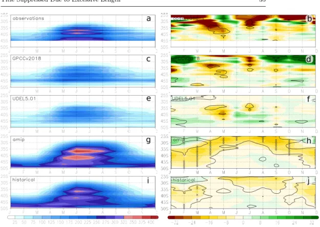
of the annual mean P-E obtained from the ensemble-mean historical simulations
559
roughly presents a hemispheric pattern that represents the ”wet gets wetter and
560
dry gets drier” paradigm of Helpd and Soden (2006) (Fig. 8a). It is worth noting
561
that the deficit of moisture supply in SWSA stands out across other extratropical
562
continental regions of the SH. The decomposition of the change of seasonal
mois-563
ture supply (Fig. 8b), reveals that changes in the atmospheric circulation account
564
for a large share of the total change compared to the direct thermodynamic effects
565
of external forcing in all seasons. Consistent with these findings, in the next
tion, we examine the potential large-scale dynamics sources associated with the
567
induced SWSA drying.
568
4.4 Connections between the HCE, SAM and SWSA rainfall
569
An anomalous shift of the circumpolar circulation in the SH high-latitudes, like
570
the one shown by the regression patterns of the undetrended PC1s of SWSA
pre-571
cipitation on circulation forcings (Fig. 6), has been related to a persistent positive
572
SAM trend and a widening of the HC in response to external forcings (e.g., Gillett
573
and Thompson, 2003; Amaya et al., 2018). The historical ensemble mean shows
574
that the seasonal low-frequency indices of SWSA precipitation, HCE and SAM
575
describe a consistent trend (left panel in Fig. 9; note that the SAM indices are
576
reversed). This trend is stronger since ∼1970s and more pronounced in DJF and
577
MAM than in JJA and SON. The square of the correlation coefficient (R2) reveals
578
high co-linearity among the three indices in all seasons (right panel in Fig. 9).
579
SWSA precipitation is almost equally correlated to HCE and SAM, showing the
580
highest co-linearity in DJF (R2= 0.87 and R2= 0.92, respectively) and the lowest
581
in JJA (R2= 0.73 and R2 = 0.74, respectively). In turn, the HCE and the SAM
582
also show a strong co-linearity between each other that is strongest in DJF (R2=
583
0.95) and weakest in JJA (R2 = 0.86). This result suggests that both dynamical
584
large-scale atmospheric modes vary in synchronously and modulate SWSA
precip-585
itation in the same direction in response to external forcings. Since both HCE and
586
SAM are highly co-linear, we next focus only on HCE index to investigate and
587
attribute the simulated trends.
588
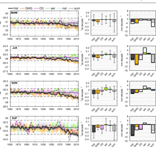
4.5 Attribution of forced variability
589
Until the early 1970s, the HCE indices of all coupled simulation oscillate around
590
the piControl climatological value and within the threshold of internal variations in
591
all seasons (Fig. 10, left panel). Afterwards, the historical ensemble-mean indices
show a poleward expansion in all seasons, even exceeding the bounds of internal
593
variations by the 2000s in JJA, SON and DJF. At the same time, the hist-nat
ex-594
periment simulates no appreciable change of the HCE variability. Such tendencies
595
evidence the role of the anthropogenic forcings on the recent HC expansion.
596
To highlight the role of external forcings, the linear trend over 1970-2014 of
597
the ensemble-mean HCE indices is analyzed (Fig. 10, middle panel). The trend
598
displayed by the historical simulation is negative, denoting a poleward expansion,
599
and significantly different from zero (with 99% confidence interval) in all seasons,
600
being even robust among all members in DJF. The expansion is widest in this
601
season with a trend of -0.20◦lat per decade, then -0.04◦lat per decade in MAM,
602
-0.07◦lat per decade in JJA and -0.11◦lat per decade in SON. Large error bars
603
evidence the great influence of internal weather noise. GHG forcing alone has a
604
large effect all year round, with a signature that emerges out of the internal noise
605
by the early 2010s in MAM and the 2000s in JJA and SON, with significant
606
1970-2014 linear trends of -0.06, -0.09 and -0.10◦lat per decade, in the respective
607
seasons. Such trend values highlight the leading role of GHGs in the HC expansion
608
during these seasons. In DJF, instead, the stratospheric ozone depletion leads the
609
HC expansion, inducing wider shift (-0.11◦lat per decade) than GHGs (-0.06◦lat
610
per decade) separately. Anthropogenic aerosols (aer) induce a significant HCE
611
equatorward shift in JJA (0.02 ◦lat per decade) and SON (0.06◦lat per decade)
612
from around the mid-1990s with a peak in the mid-2000 and a partial recovery
613
afterwards. Nevertheless, this contraction is constrained within the threshold of
614
internal variability. The 1970-2014 linear trend of the ”sum” index, obtained by
615
adding the ensemble-mean HCE anomalies from individual forcings, is significantly
616
close to the historical one (with 95% confidence interval) in DJF, MAM and JJA.
617
Therefore, the effects of the external forcings are, overall, additive all year round,
618
except in SON due to the influence of anthropogenic aerosols that tends to offset
619
the trend of the ”sum” index (-0.04 ◦lat per decade) respectively to historical
620
experiments (-0.11◦lat per decade).
To quantify the role of the HCE in the forced SWSA drying over 1970-2014,
622
we represent the total trend of SWSA precipitation from the ensemble-mean
sim-623
ulations and the HCE-coherent trend in Fig. 10 (right panel). The historical
ex-624
periment shows a precipitation reduction of 4.5, 4.4, 3.6 and 10.3 mm per decade
625
in MAM, JJA, SON and DJF, respectively, in response to all external forcings.
626
The HCE-coherent trend underestimates by 40% the total drying in MAM. Still,
627
it shows no significant difference with the total trend in the other seasons, which
628
highlights the overall leading role of the HC expansion on the drying trend induced
629
by external forcing. In MAM, in response to only GHGs the total precipitation
630
trend is significantly similar to the one induced by all forcings and is strongly
asso-631
ciated with the HC expansion. The rest of individual forcings generate no
signifi-632
cant trends. In JJA and SON, GHGs alone induce a drying trend that respectively
633
doubles and equals that caused by all forcing together and that is tightly linked
634
to HC expansion. In both seasons, ozone depletion also contributes to drying, but
635
its impact is not associated with the HCE shift. In turn, aerosols and, to a lesser
636
extent, natural forcings partially counteract the drying. Aerosols positive effect
637
on precipitation is consistent with simultaneous HC contraction in these seasons.
638
Nevertheless, the HCE index barely accounts for 23% and 18% of the total trend
639
induced by aerosols respectively in JJA and SON. In DJF, the effect of GHGs
640
and ozone depletion separately induce each around half of the trend displayed by
641
the historical simulation, while the other forcings induce no significant trend. The
642
HCE-coherent trend underestimates by 60% the drying attributed to GHGs but
643
accounts for the entire trend induced by ozone depletion. The difference between
644
the ensemble-mean trend of the ”sum” index of SWSA precipitation and the one
645
from the historical simulation suggest that the effects of individual forcings are
646
barely additive. Nevertheless, this difference is not statistically significant with
647
high significance interval, due to the considerable uncertainty among individual
648
members.
5 Discussion
650
5.1 The role of the IPO
651
Our results highlight the leading role of the SAM and the HCE on the recent
652
SWSA long-term drying trend in response to anthropogenic forcings. This is in
653
line with Boisier et al. (2018)’s finding showing that GHGs and the ozone
de-654
pletion drive the SWSA drying trend over 1960-2016 in association with positive
655
SAM anomalies. Nonetheless, Boisier et al. (2016) concludes that the forced
dry-656
ing trend at multidecadal scale can be substantially modulated by internal SST
657
variability through the IPO. This previous work focuses on the 1979-2014 period
658
and concludes, based on a linear regression model, that approximately 40% of the
659
SWSA drying trend is attributable to the concurrent pronounced negative trend
660
in the IPO index (Fig. 3). This statement opposes our result on the decomposition
661
of the decadal variance of SWSA precipitation, which reveals little influence of the
662
IPO compared to external forcing (Fig. 7).
663
To shed light on this discrepancy, we focus on the IPO-coherent trend of
pre-664
cipitation over 1979-2014 using the ensemble-mean amip-hist precipitation (upper
665
panel in Fig. 11). This trend exceeds the one attributable only to the internal
vari-666
ability of observed SST (i.e., the trend of ensemble-mean amip-hist precipitation
667
minus the trend from the historical ensemble mean) in all seasons. This diagnostic
668
evinces that a linear regression model can mislead the IPO signal on the SWSA
669
precipitation with the trend associated with external forcing. On the other hand,
670
the amip-hist ensemble-mean 1979-2014 drying trend notably exceeds the forced
671
component represented by the ensemble mean of the historical coupled runs. This
672
may suggest that the linear evolution of observed SST in 1979-2014,
character-673
ized by a steep negative IPO phase-shift, has a major contribution to the drought
674
along with external forcing. Nevertheless, the amip-hist ensemble-mean
precipita-675
tion trend may also represent an amplification of the forced drying by non-linear
air-sea interactions and atmospheric processes rather than the signature of the
677
specific IPO phase-shift.
678
To further assess whether the IPO phase shifts can directly induce decadal
679
trends in the simulated SWSA precipitation, we perform PDFs of the
precipita-680
tion trend over 1979-2014 and across all other possible 36-year periods since 1870
681
(bottom panel in Fig. 11). We use all the amip-hist members separately and
rep-682
resent the precipitation trend only in 36-year periods in which the IPO presents a
683
phase shift and significant linear trend. 50 IPO trend values are obtained, equally
684
distributed between positive and negative shifts ranging between ±0.09◦ C per
685
decade centered on respective means of 0.17◦ C and -0.16◦ C per decade. Then
686
the precipitation trend values are classified according to whether the shift is from
687
a negative to a positive IPO phase (red bars) or vice versa (blue bars).
Accord-688
ing to a two-sample t-test, the null hypothesis that the red and the blue PDFs
689
show normal distributions with equal means and variances cannot be rejected,
690
considering low confidence intervals (p>0.92) in all seasons. Their means,
repre-691
sented by the red and blue solid vertical lines, show weak changes compared to
692
the ensemble-mean trend over 1979-2014 (green solid lines; corresponding to an
693
IPO shift of -0.21◦ C per decade). But they are negative in all cases, except in
694
MAM where the blue line indicates an almost null positive trend (0.2 mm per
695
decade). Therefore, these results suggest no significant relationship between the
696
linear trend of the simulated precipitation and the sign of the IPO phase shifts
697
over 36-year periods.
698
This conclusion is supported by similar PDFs performed using the 32 historical
699
members (not shown). The resulting PDFs are not significantly different between
700
each other and to the previous ones from the amip-hist simulations, according to
701
a two-sample t-test. In addition, the resulting mean trends (red and blue dashed
702
vertical lines in Fig. 11) are weaker than the drying represented by the historical
703
ensemble mean over 1979-2014 in all seasons (green dashed lines) but negative
in most cases, consistently with the amip-hist simulations, or positive but almost
705
zero in JJA.
706
In contrast, the same analysis applied to trends over 20-year or shorter
peri-707
ods across the amip-hist simulations reveals a break up between the red and blue
708
PDFs (not shown). They show prevailing positive (negative) rainfall trends
con-709
current with positive (negative) IPO phase shifts. This means that the amip-hist
710
simulations can reproduce SWSA precipitation trends in response to IPO phase
711
shifts at intradecadal-to-decadal time scales, in agreement with other works based
712
on instrumental data (Masiokas et al., 2010). However, at multidecadal-to-longer
713
timescales, such as the 36-year-long negative IPO trend observed since the 1979,
714
the simulated effect of the IPO over the last century and a half vanishes and
715
becomes insignificant compared to the leading role of external forcings.
716
In summary, our results show that the IPO explains little variance of SWSA
717
precipitation multidecadal variability over the last century and a half, compared
718
to external forcings. However, during 1979-2014 the simulated SWSA drying trend
719
attributable only to internal variability of observed SST accounts for a large part of
720
the total trend (Fig. 11). Therefore, we can conclude that the IPO is not a leading
721
cause of long-term variability of SWSA precipitation, but it can contribute to
722
amplify forced drying trends.
723
It has to be considered that the methodology used in this work is conditioned
724
by the IPSL-CM6A-LR model biases in the atmospheric circulation. Therefore,
725
the IPO influence on SWSA precipitation long-term variability should be assessed
726
in the multi-model framework of CMIP6 to strengthen this conclusion.
727
5.2 The simulated HC expansion
728
Regarding the simulated seasonality in HCE, model trend values are comparable
729
with those from observations, with simulations reproducing a poleward expansion
730
over recent decades. In agreement with Hu et al. (2011, 2018) and model-based
731
studies (Staten et al., 2012; Hu et al., 2013; Grise et al., 2018), the HCE
sion shows strong seasonality, being larger in austral summer (DJF) than in other
733
seasons. Nevertheless, it is difficult to constrain a precise widening rate of the
734
HCE expansion due to the large spread among the trends from reanalyses and
735
the ensemble simulations. Regarding the wide range of trend values resulting from
736
the simulated ensemble members, it can be inferred that some part of the large
737
uncertainty is attributable to internal variability. In turn, observed and simulated
738
trends are comparable when the internal variability is considered, suggesting that a
739
large part of the observed HCE expansion is accounted for by internal atmospheric
740
variability (Grise et al., 2018). On the other hand, there is also large discrepancy
741
in the HCE expansion rates derived from the different reanalyses. Apart from
dif-742
ferences associated with distinct assimilation methods and model biases, this large
743
discrepancy has been attributed, in part, to shortcomings regarding the
conserva-744
tion of mass in the meridional mean circulation (Davis and Davis, 2018), especially
745
in old generation reanalyses (Grise et al., 2019).
746
5.3 HCE and SAM co-linearity
747
Our results show strong co-linearity between the SAM, HCE and SWSA
precip-748
itation, evidencing that both modes induce changes on precipitation in the same
749
direction. Furthermore, the simulated SAM strengthening and the HCE expansion
750
are attributed to the same external forcings. This suggests a connection between
751
circulation changes in tropical and high latitudes through a link of both
vari-752
ability modes under the effect of external forcing, in agreement with previous
753
works (Thompson and Wallace, 2000; Previdi and Liepert, 2007). GCMs
simu-754
late an anomalous rise of the extratropical troposphere in association with the
755
SAM strengthening (Previdi and Liepert, 2007) and the expansion of the HCE
756
(Lu et al., 2007) in future projections that consider strong external forcing effects.
757
These anomalies are related to the increase of atmospheric static stability, which
758
in turn is associated with a poleward expansion of the tropospheric baroclinicity.
759
Subsequently, there is a shift in the same direction of the hemispheric circulation
such as the westerly jets, which involves changes in both the SAM (Thompson
761
et al., 2000) and the HCE (Staten et al., 2019), and in the mid-latitude
storm-762
tracks modulating the SWSA precipitation. Nevertheless, the factors that control
763
the extratropical atmospheric static instability are still unknown and, by
exten-764
sion, the mechanisms that explain the link between changes in the SAM and the
765
HCE.
766
5.4 The role of anthropogenic forcing
767
Our results show that anthropogenic forcings have largely induced the recent
768
SWSA drying through dynamical changes associated with the HCE and SAM.
769
GHGs play the leading role on the HC expansion and the subsequent SWSA
dry-770
ing trend all year round except in DJF. In this season, the effect of GHGs is
771
combined with the ozone depletion, which is the dominant factor. Although not
772
shown in this paper, the leading effects of GHGs and ozone depletion are found to
773
be similar on the HCE and the SAM. We also find that the effect of anthropogenic
774
aerosols can offset the simulated HC expansion and the SWSA drying trend over
775
1970-2014. This is most likely related to the counteracting effect of aerosols on the
776
global warming induced by GHGs (Andreae et al., 2005). However, the HC
con-777
traction barely explains a fraction of the forced rainfall increase, which is largest in
778
JJA (Fig. 10) coincident with positive thermodynamics of the P-E imbalance (Fig.
779
8). This suggests that aerosols may induce precipitation changes in SWSA through
780
thermodynamical processes. Nevertheless, aerosols effects are highly uncertain and
781
poorly constrained by climate models (Andreae et al., 2005; Boucher et al., 2013;
782
Carslaw et al., 2013; Oudar et al., 2018), suggesting that further investigation
783
should be done to shed light on this concern.