Design and optimization of micropumps using electrorheological and magnetorheological fluids

Design and Optimization of Micropumps Using

Electrorheological and Magnetorheological Fluids

by

Youzhi Liang

Submitted to the Department of Mechanical Engineering in partial fulfillment of the requirements for the degree of

Master of Science in Mechanical Engineering

at the

MASSACHUSETTS INSTITUTE OF TECHNOLOGY

ARCHIVES

MASSA CHUSETTS INSTITUTE

OF LCHNOLOLGY

JUL 3

02015

LIBRARIES

June 2015

@

Signature redacted

Author ... ...

Department of Mechanical Engineering

May 18, 2015

Certified by...

Signature redacted

....-...-.

Karl Lagnemma Principal Research Scientist Thesis Supervisor

Signature redacted

A ccepted by ... ... . ... ...

David E. Hardt Chairman, Department Committee on Graduate Theses

MITLibraries

77 Massachusetts Avenue Cambridge, MA 02139

http://Iibraries.mit.edu/ask

DISCLAIMER NOTICE

Due to the condition of the original material, there are unavoidable flaws in this reproduction. We have made every effort possible to

provide you with the best copy available. Thank you.

The images contained in this document are of the best quality available.

Design and Optimization of Micropumps Using

Electrorheological and Magnetorheological Fluids by

Youzhi Liang

Submitted to the Department of Mechanical Engineering on May 18, 2015, in partial fulfillment of the

requirements for the degree of

Master of Science in Mechanical Engineering

Abstract

Micropumps have rapidly expanded microhydraulic systems into a wider range of ap-plications, such as drug delivery, chemical analysis and biological sensing. Empirical research has shown that micropumps suffer most from their extremely low efficiency. To improve the efficiency of micropumps, we propose to employ electrorheological (ER) and magnetorheological (MR) fluids as the hydraulic fluids. This thesis presents two methods: one is a dynamic sealing method to be applied on current micro-scale gear pumps using MR fluids, and the other is a novel design method of micropumps using ER fluids.

Using MR fluid with applied magnetic field as a substitute for industrial hydraulic fluids, magnetic chains are aligned within the channel. The parameters, such as magnetic field, viscosity and volume fraction of MR fluid can be balanced to provide optimal sealing performance. Darcy flow through porous media and Bingham flow in a curved channel with a rectangular cross section have been used to model the MR fluid flow exposed to certain magnetic field intensity. Static and dynamic magnetic sealing performance is investigated theoretically and experimentally, which is evaluated by Mason numbers and friction factor.

To achieve a higher efficiency and faster dynamic response, a novel design for micropumps driven by ER fluid is demonstrated. Moving mechanical parts are elim-inated by applying a periodic voltage gradient. The approach involves exerting elec-tric forces on particles distributed within the fluid and exploiting drag or entrainment forces to drive flow. Variables are explored, such as the dimension and layout of the channel and electrodes. Experiments are also designed to observe the performance of the solid state pump. In addition, a method of characterizing the efficiency of cham-ber pump is introduced and applied on screw-chamcham-ber pump and solenoid-chamcham-ber pump with check valve and ER valve.

Thesis Supervisor: Karl Iagnemma Title: Principal Research Scientist

Acknowledgements

I would like to sincerely express my gratitude to my advisor, Karl lagnemma for his

invaluable guidance, mentorship and inspiration. This thesis has benefited greatly by his profound knowledge, in the areas of, amongst many others, design principle of micro-scale pumps. I am thankful to Professor Anette Hosoi for her insight into fluid mechanics and precious advice. I would like to thank Regan Zane and Michael Evzelman for their expertise in the field of electrics and circuits.

I am grateful for the effort and encouragement provided by Jose Alvarado. He

is the friend whom I want to turn to for help when I got stuck in a problem and to share with when accomplishment was achieved. I would like to thank Jean Comtet and Matthew Demers for their insight into my work. I wish to thank Marie Helence Baumier for her initial contributions to the study of dynamic sealing.

I would like to thank all the colleagues in Robotic Mobility Group and in

Hatsopoulos Microfluids Laboratory. This thesis could not be finished without their help on the analysis of my work and their guidance on the apparatus operation.

Special thanks to Yongkang Ma for his support, positive and negative encouragement and his tolerance. I thank my parents for their love, sacrifice and

understanding, for which I am forever grateful and more than I could ever hope to repay.

Contents

1

1.1 M icropum ps ... 16

1.2 Electrorheological and Magnetorheological Fluids ... 19

1.3 G oals ... 20

2 Optimization of Pumps Driven by Magnetorheological Fluid 23 2.1 Background ... 23

2.2 Magnetorheological Sealing Experiment Design ... 23

2.2.1 Mechanical Structure ... 23

2.2.2 Electrical Connection ... 26

2.2.3 Magnetic Field ... 27

2.3 Models for Flow in Curved Channels with a Rectangular Cross Section .29 2.3.1 Couette Flow in Curved Rectangular Cross Section Channels. . 29 2.3.2 Poiseuille Flow in Curved Rectangular Cross Section Channels. 34 2.3.3 Bingham Flow for Magnetorheological Fluid ... 39

2.3.4 Darcy Flow for Magnetorheological Fluid ... 41

2.4 Static Performance ... 42

2.4.1 Performance under Poiseuille Flow ... 43

2.4.2 Performance under Couette Flow ... 46

2.5 Dynamic Performance ... 47

2.5.1 Hydraulic Performance ... 47

2.6 Discussions and Evaluations ... 49

2.6.1 Dimensional Analysis ... 49

2.6.2 Evaluation by Friction Factor and Mason Number ... 50

3 Design of Pumps Driven by Electrorheological Fluid 53 3.1 Background ... 53

3.2 Chamber Pumps ... 54

3.2.1 Design of Screw-Servo Chamber Pump ... 54

3.2.2 Evaluation of Servo Motor Performance ... 55

3.2.3 Evaluation of Hydraulic Performance ... 57

3.2.4 Efficiency Evaluation with Electrorheological Valve ... 58

3.3 Solid State Pumps ... 59

3.3.1 Design of the First Prototype ... 59

3.3.2 Design of the Second Prototype ... 62

3.3.3 Simulation and Experiments ... 63

4 Conclusions and Future Work 67 4.1 Conclusions ... 67

List of Figures

1-1 Review of efficiency versus maximum pressure for existing small-scale pumping strategies. The different shades denote mechanical or non-mechanical pumps. The size of the symbol depicts the characteristic length scale of the pump package. For reference, Sim et. al. is 72 mm3 and Kargov et. al. is 18.5 cm3 . . . . . 18

2-1 A picture of experimental setup. 1: Motor, 2: Frame, 3: Disk, 4: Channel, 5: Pitot tube, 6: Scaled plate, 7: Magnet, 8: Spacers... 24

2-2 A schematic of flow formation. The flow bifurcates into two branches

exposed to different magnetic field intensity. A Couette flow rate is also induced by a rotating disk... 25 2-3 A schematic illustration of the electric network of the experimental

setup... 27

2-4 Magnetic field intensity distribution along the circular channel. The magnet is 70 mm away from the circular channel with a diameter of 100 m m ... 28

2-5 A schematic illustration of the flow in a form of Couette flow in a circular

channel with rectangular cross section... 30

2-6 A schematic illustration of the circular Couette flow. The viscous fluid

flows in the gap between an inner cylinder with radius R1 that rotates at

angular speed Q1 and an outer cylinder with radius R2 that rotates at

2-7 Velocity and pressure distribution for concentric rotating cylinder. (a) Velocity distribution. (b) Pressure distribution. Two dimensionless quantities are evaluated by the ratio of the relative value and the span. .. 32

2-8 Schematics for Couette flow between parallel plates. (a) Couette flow between infinite parallel plates. (b) Couette flow between parallel plates limited by two static parallel boundaries... 33

2-9 Velocity distribution. Dimensionless quantities are evaluated by the fraction...34

2-10 A schematic illustration of the circular Poiseuille flow. The viscous fluid flows in the rectangular cross section channel, which is driven by pressure

gradient (PI -P 2)/7r. ... 35

2-11 Schematics for Poiseuille flow between parallel plates. Flow is driven by pressure gradient from P1 to P2. (a) Poiseuille flow between infinite

parallel plates. (b) Poiseuille flow between parallel plates limited by two static parallel boundaries... 36

2-12 Velocity distribution. Dimensionless quantities are evaluated by the

fraction...38 2-13 Viscosity measurement. Pressure differential (psi) as a function of flow

rates (mL/min). Each point corresponds to the mean from three iterations of experiments, with error bars indicating standard deviation... 39 2-14 A schematic illustration of the Bingham flow model. (a) Newtonian flow

through parallel plates. (b) Bingham flow through parallel plates... 41

2-15 Viscosity measurement. Pressure differential (psi) as a function of flow

rates (mL/min). Each point corresponds to the mean from three iterations of experiments, with error bars indicating standard deviation. The experiments without magnet was conducted with known viscosity

2-16 Deformation of magnetic chains for different flow rates (Channel width: 0.7 mm, viscosity: 1.78 Pa-s, MR fluid volume fraction: 10%). Flow rates

from (a) to (i): 0.01 mUmin, 0.1 mL/min, 1 mL/min, 5 mL/min, 10 mL/min, 15 mrLmin ... 44

2-17 Pressure differential (psi) as a function of flow rate (mLlmin), for channel

widths from 0.5 mm to 0.9 mm. Each point corresponds to the mean from three iterations of experiments ... 45

2-18 Deformation of magnetic chains for rotational speed (Channel width: 0.7

mm, viscosity: 0.97 Pa-s, MR fluid volume fraction: 1%). Rotational speed from (a) to (c): 0 rps, 0.4 rps, 0.8 rps... 47

2-19 Dynamic sealing performance. Pressure differential (psi) as a function of

rotational speed (rps), for flow rates from 0.1 mL/min to 0.8 mL/min. Each point corresponds to the mean from three iterations of experiments, with error bars indicating standard deviation... 49 2-20 Power dissipation. Power input (mW) as a function of rotational speed (rps), for flow rates from 0.1 mUmin to 0.8 rmL/min. Each point corresponds to the mean from three iterations of experiments ... 50

2-21 Hydraulic performance evaluated by Friction factor. The ranges of the three dimensionless groups in the figure are scaled down from 0 to 1. . 52 2-22 Hydraulic performance evaluated by Mason #2. The ranges of the three

dimensionless groups in the figure are scaled down from 0 to 1 ... 52

3-1 (a) A picture of the chamber pump. (b) Sectional view of the 3-D model of the chamber pump with one quarter removed. 1: Guider, 2: Plunger, 3:

Gasket, 4: Diaphragm, 5: Chamber, 6: Screw, 7: Servo... 55

3-2 A picture of the chamber pump driven by solenoid... 56

3-3 Power input versus time. The voltage ranges from 3.0 V to 12.0 V. One cycle of 10 s is shown in the figure... 57

3-4 Experimental setup for the evaluation of hydraulic performance. Texture Analyzer was implemented to control the distance and velocity of the

plunger...58

3-5 Hydraulic efficiency. The distance of plunger exerted on the diaphragm ranges from 2 mm to 8 mm. The velocity indicates the speed of plunger. 59

3-6 A picture of the solid state pump. (Channel width: 0.5 mm, Electrodes

width: 0.7 mm, Electrodes spacing: 0.3 mm.) ... 61 3-7 Exploded view of the 3-D model of the solid state pump. 1: Upper plate, 2:

Tube fitting, 3: Electric connector, 4: Printed circuits, 5: Electrodes, 6: M iddle plate, 7: Lower plate... 61 3-8 A schematic of the channel. Different variables have been explored:

electrode width: 0.7 mm, 0.9 mm, 1.2 mm; spacing: 0.5 mm, 0.7 mm, 0.9 mm; channel width: 0.3 mm, 0.5 mm, 0.7 mm. Eight pairs of electrodes, wrapped around the middle plate, are equally distributed along the

channel...62 3-9 A picture of the solid state pump with pitot tubes to evaluate pressure

differential. (Channel width: 0.5 mm; Electrodes width: 0.7 mm; Electrodes spacing: 0.3 mm.)... 63 3-10 3-D model of the second prototype solid state pump. 1: Printed circuit

board, 2: Tube fitting, 3: Upper plate, 4: Middle plate (with a circular channel), 5: Lower plate ... 64

3-11 A typical voltage gradient. The number indicates the voltage (V) on each

electrode. (Image was provided by Matthew Demers.) ... 65

3-12 Particle aggregation simulation with the channel. The small black dots

indicate the dipole particles. (Image was provided by Matthew Demers.)65

3-13 Experimental setup to observe solid particle movement in the channel

3-14 A sequence of pictures of the solid particle movement. (Image was provided by Michael Evzelman.) From (a) to (f), it shows the particles within the channel at t = 1 s, 6 s, 11 s, 16 s, 21 s, 26 s. (Image was provided by Michael Evzelman.) ... 66

List of Tables

2-1 Viscosity Measurement for Gelest Silicone Oil IOOcSt ... .38

2-2 Viscosity Measurement for MR Fluid ... 40

3-1 Efficiency of the servo motor. (Voltage U (V) and current I (A) was acquired directly from the power supply. Distance h (m) was defined by the height of the weight, which was lifted by the servo. ) ... 51

Chapter 1

Introduction

1.1

Micropumps

Micropumps are defined as miniaturized pumping devices by micromachining technologies from the perspective of MEMS [1, 2]. The earliest reported concept of a micropump can be dated back to 1975, mainly consisting of a variable volume chamber, piezoelectric benders and solenoid valve for implantation into human body [2]. After this pioneering work, the concept was oriented towards the MEMS field around 1990 [3]. In recent years, the potential target applications have been widely expanded due to novel physical principles and fabrication methods. Micropumps are commonly used in chemical analyses, biological sensing, and drug delivery [4-6].

Micropumps can generally be classified into two categories: mechanical pumps and non-mechanical pumps. In terms of actuation principles, the most common mechanical methods include piezoelectric [6-8], bimetallic [1], thermopneumatic

[9-11], electrostatic [3], electromagnetic actuation [3] and shape memory alloy

(SMA) [12-14]; the most common non-mechanical methods include

magneto-hydrodynamic (MHD), electro-hydrodynamic (EHD), and electro-osmotic actuation. The most widely used microactuation techniques are summarized in the following with advantages and disadvantaged discussed.

This actuation concept is based on the piezoelectric effect which correlates mechanical deformation and electrical polarization [1]. Due to the fast response and precise dosage, piezoelectric micropumps are commonly used to maintain therapeutic efficacy, such as drug delivery [4, 5]. However, the drawbacks for the piezoelectric micropumps are considered to be the high actuation voltage and the mounting procedure [3].

Thermopneumatic micropumps are designed by a periodic change in the volume of the chamber expanded and compressed by a pair of heater and cooler [1]. Micromachining, either for the heater and cooler or the diaphragm, contributes to the realization of this principle [9-11]. The crucial disadvantages for thermopneumatic micropumps is the long thermal relaxation time constant of the cooling process which will limit the bandwidth of the actuation [3], and the driving power which is required to be maintained at a specified-constant level [1].

The shape memory alloy (SMA) micropumps generally refer to those applying the shape memory effect (SME) of SMA among which Titanium/Nickel (TiNi) are most commonly used as being capable of high actuation forces and high recoverable strains, resulting in large pumping rates and high operating pressures [12-14]. The main disadvantages are the relatively high power consumption indicating a low efficiency and the uncontrollable deformation of SMA due to its temperature sensitivity [1].

Considering the efficiency of microhydraulic systems, all types of pumps introduced above suffer from a low efficiency. Typically, the overall efficiency of a micropump is determined by the product of four components: volumetric efficiency, hydraulic efficiency, mechanical efficiency and electrical efficiency. Volumetric losses and hydraulic losses dominate at small scales, although an acceptable efficiency for macropumps has already been achieved. As the size of the system decreases, the volumetric efficiency is dramatically affected since the same

dimensional and geometric tolerance result in a larger dimension fraction. In terms of hydraulic efficiency, Reynolds number also decreases as the characteristic length scales decreases, leading to larger viscous losses.

10

-i 10

Krg gov et. al.

..7-7xojea e...a....

Ri hter et. al.

)Schomb rg et. al. (1994) (20 8) \an de Pol et. al.

Sim et. al. ___ Mech mical

8.(2003)... al.0(2002)

(2005)

1-;;m,+

11

1

111E

1

51

0.1 1 Pmax (kPa)

Figure 1-1: Review of efficiency versus maximum pressure for existing small-scale pumping strategies. The different shades denote mechanical or non-mechanical pumps. The size of the symbol depicts the characteristic length scale of the pump package. For reference, Sim et. al. is 72 mm3 _{and Kargov et. al. is 18.5 cm}3_{. The}

type of each pump is specified as the following: Sim et. al: Micropump with flap valves [15], Kim et. al: Electromagnetic pump [16], Yun et. al: Surface-tension driven pump [17], Richter et. al: Electrohydrodynamic pump [18], Tsai et. al: Thermal-bubble-actuated pump [19], Kargov et. al: Gear pump [20], Grosjean et. al: Thermopneumatic pump [21], Schomburg et. al: Pneumatic chamber pump [22], Van de Pol et. al: Thermopneumatic pump [23], Zengerle et. al: Electrostatic pump [24], Shen et. al: Electromagnetic pump [25], Yao et. al: Electroosmotic pump [26], Reichmuth et. al: electrokinetic pump [27].

The efficiencies of reported available micropump technology are shown in Fig. 1-1. The efficiencies of all of most micropumps are less than 1 percent. Especially at low pressure, the efficiency is quite low. The rectangular area indicates the target area of the design of our micro-pumps. Our goal is to build micropumps at low flow rate with a higher efficiency.

1.2

Electrorheological (ER) and magnetorheological

(MR) fluids

Electrorheological (ER) fluids and magnetorheological (MR) fluids are both non-colloidal fluids suspended with polarizable particles. These two fluids are capable of being transformed from the liquid state to solid state in milliseconds when exposed in electric or magnetic field [28].

Electrorheological (ER) fluids basically consist of suspended non-conducting particles, up to 100 micrometers, in an insulating fluid [29]. There has been extensive study on the mechanism of ER fluid. Water bridging and polarization of the particles are proposed to explain the shear strength of ER fluids when an electric field is applied [28, 29]. The operational mode for ER fluid can be categorized as flow mode, shear mode and squeeze mode [28]. Typical applications for ER fluids are valves [30-32], clutches [33, 34], absorbers [35, 36], and engine mounts [37, 38].

The wide range of applications benefits from the striking features of ER fluids, like fast dynamic response [32, 41, 42], facile mechanical interface connection [43, 44] and accurate controllability [41, 42]. The response time for DC and AC excitation is on the order of milliseconds, and varies exponentially with the density of the particle [28, 45]. The simplicity of the mechanical structure of the interface connection can be seen in the devices in vales and engine mounts [30-32, 37, 38].

electrorheological (ER) fluids [46]. It is initially used by Jacob Rabinow for a design of clutch in the late 1940s [47]. A commercial success has just been achieved in the recent years [46].

The typical operational mode for the application of MR fluids are pressure driven flow mode and direct shear mode [48, 49]. The most common application is damper, for its appealing features such as low-power consumption, force controllability and rapid response [51]. Especially, the damper for vehicles has been widely investigated and revealed attractive properties [52-54].

The other typical use of MR fluids is the development of MR valves. Compared with ER valves, the most evident advantage is that the apparent viscosity could be controlled by a wider applied magnetic field [55]. In addition, a high efficiency and miniaturization of MR valve have been achieved [56, 57]

Previous research primarily focuses on MR and ER fluids within the scope of high shear stress resulting in large pressure differential or large exerted force [50-57]. However, in this thesis, the low shear stress behavior and dynamic response of ER fluids are mainly studied and applied to the micropump design and micropump

sealing.

1.3

Goals

Our goal is to address the inefficiency of micropumps. We propose to employ electrorheological (ER) and magnetorheological (MR) fluids as the hydraulic fluids. In this thesis, MR fluid is investigated for dynamic sealing to be applied on current micro-scale gear pumps; ER fluid is designed to be the hydraulic fluid for a novel design of solid state pump. The theoretical and experimental results to evaluate the performance of dynamic sealing and solid state pump are also presented.

In Chapter 2, four mathematic models for fluids in a curved channel with rectangular cross section are built first, followed by the experimental results of static performance and dynamic performance. A group of dimensionless quantities are defined for the evaluation at last. Chapter 3 includes two sections. The first section discusses the characterization of the performance of chamber pumps. Two kinds of chamber pumps, screw-chamber pump and solenoid pump, are designed and evaluated by a method to characterize the efficiency. The second section elaborates the design of the structure and fabrication of solid state pumps. Experiments are also conducted to observe the performance. Finally, conclusions and future work are briefly summarized in Chapter 4.

Chapter

2

Optimization of Pumps Driven by

Magnetorheological Fluid

2.1 Background

Sealing is necessary for micropumps due to its inefficiency discussed in Chapter 1.1. The traditional sealing method for gear pumps is achieved mechanically by controlling the geometric and dimensional tolerance.

This chapter introduces a novel sealing method, applying magnetorheological (MR) fluid as the hydraulic fluid. Simplified mathematical models for a curved channel with rectangular cross section are discussed first, followed by the experimental results and evaluation of the hydraulic performance.

2.2

Magnetorheological Sealing Experiment Design

2.2.1 Mechanical structure

An experimental setup was designed to test the sealing performance with magnetic rheological fluid in terms of the effectiveness of magnetic brush deformation induced by Poiseuille flow and Couette flow. Sealing performance was observed

under the condition of different flow rates and rotational speed of the wall.

Figure 2-1: A picture of experimental setup. 1: Motor, 2: Frame, 3: Disk, 4: Channel,

5: Pitot tube, 6: Scaled plate, 7: Magnet, 8: Spacers.

As shown in Fig. 2-1, the experimental setup mainly consists of frame, motor, disk, pitot tube and magnet. The frame is designed to secure other components; actually, there is a cavity inside of it, which connects tube fitting, the pitot tube and the tube connected with the disk in the middle. We have built a micro-channel network as Fig. 2-2 shows. A laser cut acrylic sheet was sandwiched between two transparent plates with slots to locate magnets. Spacers are designed to modulate the magnetic field

intensity in either channel.

MR fluid flows along the path as the arrow denotes in Fig. 2-2. By exerting magnetic field, magnetic brushes are formed along the channel so that pressure can be hold back. Flow bifurcates into two channels: one channel is exposed to higher magnetic field intensity, which will be treated as a porous media, resulting in a higher fluid resistance; the other one is modeled as Bingham flow due to a lower magnetic field intensity.

To mimic the flow in the gap of gear pumps, one magnet was designed so that stronger magnetic field density could be exerted on the channel where the direction of the flow caused by pressure differential was reverse to that of the Couette flow. Spacers were used to adjust the magnetic field intensity inside of the channels.

Porous media Disk Flow i DR Flow OR Darcy flow

Figure 2-2: A schematic of flow formation. The flow bifurcates into two branches

exposed to different magnetic field intensity. A Couette flow rate is also induced by

a rotating disk.

The carrier fluid of the MR fluid is Gelest silicone oil 100cSt. MR fluid accounts for

10 percent in volume fraction. The magnets are designed to be quite strong, with a

surface field of 1895 Gauss (NdFeB, Grade N42, 2.44 oz.).

Flow rate was controlled by high pressure syringe pumps, ranging from 0.1 mI~min to 0.8 mI~min. The rotational speed of the wheel is set by a DC motor (Pololu 12V) with a variable-voltage power supply and measured via an encoder on the motor.

Pressure at the inlet and outlet of the setup was designed to be measured by both pressure sensors and pitot tubes. Pitot tubes were primarily used to calibrate the

sensors, since the pitot tube was subject to the dynamic response of the fluid, indicating a longer period of time to get stabilized ( In the experiment, it took 90 minutes to calibrate sensors).

Experiments were conducted under the condition of flow rates from 0 m/min

to 0.8 m/min with different rotational speed from 0 rps to 1 rps for three iterations.

The magnetic sealing performance was observed and evaluated statically and dynamically.

2.2.2

Electrical Connection

Electric network for the experimental setup is shown in Fig. 2-3. A variable-voltage power supply was used to power both the sensors and the motor, using voltage 10.5 V and from 0 V to 40 V respectively. Data acquired from the sensors were sent to Labview via National Instruments 1/0. Arduino was employed to acquire speed feedback from the encoder on the motor.

Aluminum foil was designed to isolate pressure sensors to screen the signal noise from the motor, the power supply and also the strong magnets. The aluminum foil was also grounded with the minus for the sensors and the motor together.

Power Supply Liquid IN --- Minus -- Plus Twisted - - sensor I Foil

G round Point Channel

GND

g Inputs Aluminum Foil

National Instruments I/O

Lqdsesor

Liquid OUT GND

Pair

Figure 2-3: A schematic illustration of the electric network of the experimental setup.

2.2.3

Magnetic Field

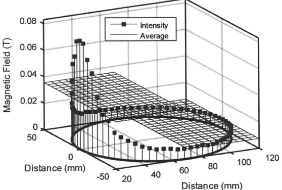
Shear stress of the MR fluid in presence of magnetic field was determined by the intensity of it besides the volume fraction of the MR fluid in our experiments. The magnetic field intensity was measured by Gauss meter along the circular channel, as shown in Fig. 2-4. For a dipole, theoretically, the intensity decreases by the radius to the third power in Equation (2.1), which indicates the distance between the dipole and the location being measured.

B(m, r,A)=- -11+3sin22,

where B is the strength of the field, r is the distance from the center, A is the magnetic latitude, m is the dipole moment, po is the permeability of free space.

Our measurement results show that the magnetic field intensity drops abruptly, and then keeps almost constant. The two (red) planes in Fig. 2-4 denotes the average intensity for the right half circle and the left half one respectively, indicating that the branch immediate to the magnet is 3.8 times larger than that on the further end. Taking the magnetic field direction into account, the intensity within the right further half circle will decrease to 50 % because of a field direction normal to the

channel for a large part. This magnetic field intensity distribution lays the foundation for the different mathematical models of the two channels.

0.08 _{- Intensity} Averae S0. 06 Uj-0.04 0.02 0 50 0 120 Distance (mm) 60 80

-50

20

40

Figure 2-4: Magnetic field intensity distribution along the circular channel. The magnet is 70 mm away from the circular channel with a diameter of 100 mm.

2.3 Models for Flow in Curved Channels with a

Rectangular Cross Section

2.3.1 Couette Flow in Curved Rectangular Cross Section Channels

We consider two concentric rotating cylinders with angular speed of Q, and Q2

respectively, which are limited by two parallel plates with height h, as Fig. 2-5 shows. This structure forms a rectangular cross-section curved channel. Along the channel, there is no pressure gradient. We employ cylindrical coordinates (r,(p,z), with the z-axis coinciding with the axis of the center line of the cylinders. By applying Navier-Stokes equation, the only non-zero component of velocity is the angular velocity u,(rz). This velocity distribution automatically satisfies the continuity equation. The angular equation of motion reduces to

Fa i

1

a

_u,

_{(r, z)l}

O=p (ru,

(r,

ar _ r ar I Z2

Non-slip condition:

U9,(RI)=QIRI,

u,(R

)

u,(z=h/2)=O, u,(z=-h/2)=O.

Z R, R, DR V-0 -(22R22R2 SV=0 2R DIRI

Figure 2-5: A schematic illustration of the flow in a form of Couette flow in a

circular channel with rectangular cross section.

(a) Steady Flow between Concentric Rotating Infinite Cylinders

A schematic illustration of the steady flow between concentric rotating infinite

cylinders is shown in Fig. 2-6.

Figure 2-6: A schematic illustration of the circular Couette flow. The viscous fluid flows in the gap between an inner cylinder with radius R1 that rotates at angular

speed Q, and an outer cylinder with radius R2 that rotates at angular speed Q2.

Using cylindrical coordinates and assuming that u = (0, u,(r), 0), the continuity equation is automatically satisfied, and the momentum equations for the radial and tangential directions are the following:

U. (r - , (2.4)

r p dr

0=r7dI

(

(r)),

dr r dr

where p is the density of the fluid (units: kg m-3), I is the viscosity (units: Pa s). Initial conditions:

Substitution of Equation (2.6) into Equation (2.5) produces the velocity distribution:

u,(r)2= 2] {[₂Ri -Q₁R]r-[02 - 01

}

(2.7)

RU- QII rf,2

When the outer cylinder is static, Equation (2.6) reduce to

1(r)= -r+-R (2.8)

R - RI r

Substituting u,(r) into Equation (2.4) give us the pressure distribution, assuming the initial condition is the atmosphere:

P - P = p2

1-4R; In

r R 2_R2 2 2 R, R2

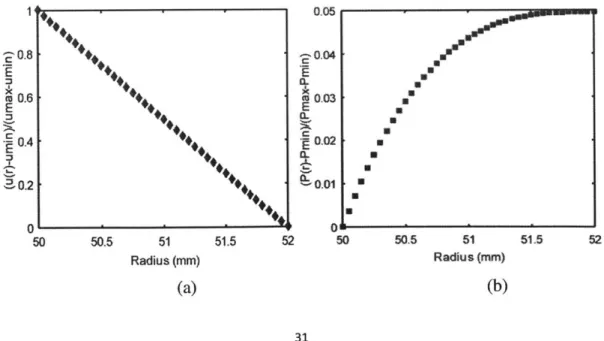
Fig. 2-7 (a) suggests that although u,((r) derived from the nonlinear Equation (2.8), the velocity distribution within R1 = 50 mm and R2 = 52 mm for our experimental setup shows a nice linearity. The pressure distribution, shown in Fig. 2-7 (b), can be treated as a constant along the channel, since the largest differential of the pressure is less than 5 %. These two distributions are quite similar to the condition for laminar flow in two parallel plates. Therefore, the loss for a concentric rotating cylinder can be simplified as the loss for two parallel plates with the same geometry

and dimension. ii,, 0.05 -0.8 -0.04 0.6 0.03 E :0-50 50.5 51 51.5 52 50 505 51 51.5 52 Radius (mm) Radius (mm) (a) (b)

Figure 2-7: Velocity and pressure distribution for concentric rotating cylinder. (a) Velocity distribution. (b) Pressure distribution. Two dimensionless quantities are evaluated by the ratio of the relative value and the span.

(b) Steady Flow between Parallel Plates

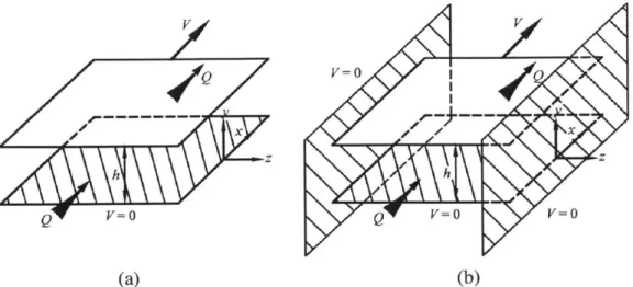
The average velocity for Newtonian viscous flow between two parallel plates is 0.5V, as shown in Fig. 2-8 (a), while limited by another two parallel plates, the average velocity reduces to 0.19V, as shown in Fig. 2.8 (b).

The boundaries are considered to exert a linear decrease on the initial velocity distribution. A clearance 6, as shown in Fig. 2-5, is necessary to take into account otherwise two singular points at the corner of the moving plate will occur because of an infinite velocity gradient. Given the specific experimental setup as described in Chapter 2.1, velocity distribution within a squared area is calculated to be 0.19 V as

shown in Fig. 2-9.

Therefore, the average velocity of the flow between two concentric rotating cylinders is given by R-, fu , (r)rdr - QR2 R U O R r+ R2rdr R2 -R1

(R)

V=V V= V= (b) h dV v=o (a)

Figure 2-8: Schematics for Couette flow between parallel plates. (a) Couette flow between infinite parallel plates. (b) Couette flow between parallel plates limited by two static parallel boundaries.

1~ 0.81 0.6. E 0.4 0.2 0. 0 -0.5 (r-RI)/(R2-RI)

₁

hAi

Figure 2-9: Velocity distribution. Dimensionless quantities are evaluated by the fraction.

2.3.2 Poiseuille Flow in Curved Rectangular Cross Section Channels

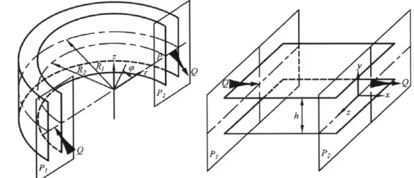
We attempt to approach the solution in a simpler method to the real velocity distribution of the Poiseuille flow in a curved rectangular cross section channel by diving it into three steps: to solve for the velocity distribution of Poiseuille flow in a channel between two concentric infinite cylinders; to solve for the velocity distribution of the Poiseuille flow in a channel between two parallel infinite plates; to substitute the velocity distribution between cylinders into that between plates as the peak. A schematic illustration of the circular Poiseuille flow is shown in Fig. 2-10.

/ R, 1 r P2 Q

h,

Figure 2-10: A schematic illustration of the circular Poiseuille flow. The viscous fluid flows in the rectangular cross section channel, which is driven by pressure gradient (PI -P 2)/xr.

Assuming that u = (0, u,(r), 0), the Navier-Stokes equation in the tangential

direction written in cylindrical polar coordinates in the absence of body force is

a ia

u,(r,

z)1

0=r7(ru, (r, z)) + 2 ,

(r (2.11)

-ar r ar(

aZ

r aqp

where rq is the viscosity of the fluid, dp/ihp is (PI-P2)/.

u,(r=R,)=O, u,(r=R2)=O, u,(z=h/2)=O,

(a) Poiseuille Flow between Concentric Infinite Cylinders

A schematic illustration of Poiseuille flow between two concentric infinite cylinders

is shown in Fig. 2-11.

2, Q

'0 ~h

01P$

Figure 2-11: Schematics for Poiseuille flow between parallel plates. Flow is driven

by pressure gradient from P1 to P2. (a) Poiseuille flow between infinite parallel

plates. (b) Poiseuille flow between parallel plates limited by two static parallel boundaries.

Assuming that the tangential velocity u, is dependent of r and z, the Navier-Stokes equation reduces to

(1 I\ 1 Dlp

0=7 -

(ru,(r,z))I

ar rar rap

No slip conditions:

u,(r=R,)=O; u,,(r=R

)=O

With the initial conditions from Equation (2.14), the partial Equation (2.13) can be solved for the velocity distribution:

_1 (ap

"F

(1n

U,

(r)=

(b) Poiseuille Flow between Infinite Parallel Plates

As Fig. 2-11 (b) shows, the Poiseuille flow between two parallel infinite plates driven by pressure differential can be solved with initial conditions:

a

_u,

_ap

a=p (2.16)

O= -y 2 g

u,(z=h/2)=O,u,(z=--h/2)=0.

Velocity distribution is:

lap 2

lap/i

u(y)= y I 2(2.18)

pax pax4

Rewrite Equation (2.18) expressed by the peak:

2h2

mX

(a) x _

(r)

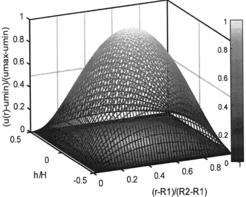
at the boundaries in a form of parabola. In addition, the velocity distribution in the r-direction remains a pattern as u,(r). Given the geometric symmetry in z-direction, the maximum velocity it can reach, if possible in terms of z-direction, must be u,(r). Therefore,

Uxma (r)=u,(r) (2.20)

Substitute Equation (2.19) into Equation (2.15):

1

ap

1R(lnR-1nR2)

uq,(r,y)= (L) rlnr- - I r + y

2p

aO

12-R

Y

(2.21) The result of the velocity distribution of the Poiseuille flow between two parallel

- 0.8 0.8 0.6

E

04

0.6

0.8

(r-RI )/(R2-R1)

Figure 2-12: Velocity distribution. Dimensionless quantities are evaluated by the fraction.

Using silicone oil with known viscosity 0.0974 Pa-s (Gelest silicone oil 100cSt; Experimental result of the measurement by rheometer is (0.09979 0.00114) Pa-s shown in Table 2-1), we conducted a group of experiments to measure the viscosity of it to verify of the mathematical model introduced above by the experimental setup as shown in Fig. 2-12. Fig. 2-13 indicates a viscosity of 0.115 Pa- s, which agrees with the specification from manufacturer very well.

Table 2-1: Viscosity Measurement for Gelest Silicone Oil IOOcSt

Shear Stress Strain Rate Viscosity

(Pa) (1/s) (Pa- s)

0.9939 9.866 0.1007

1.459 14.30 0.1020

3.143 31.06 0.1012 4.613 45.50 0.1014 6.771 68.20 0.09928 9.939 100.2 0.09923 14.59 147.1 0.09915 21.41 215.7 0.09926 31.43 315.3 0.09967 46.13 465.7 0.09906 67.71 685.0 0.09984 99.38 1010 0.09938 Mean 0.09979 Standard Deviation 0.00114 0.15 0.14 0. _0.13 0.12 o 0.11 CO, Cn 0.1 a . 0.09 A flO ---FFitting line Experimental results 0 0.2 0.4 0.6 0.8

Flow Rate (mL/min)

Figure 2-13: Viscosity measurement. Pressure differential (psi) as a function of flow rates (mL/min). Each point corresponds to the mean from three iterations of

2.3.3 Bingham Flow for Magnetorheological Fluid

A conventional model used to characterize MR fluid for simple analysis is the

Bingham plastic model, though MR fluid is also known to be subject to shear thinning, and below the yield stress, behaves as a viscoelastic material dependent on magnetic field intensity. A slight tendency of shear thinning was observed in the viscosity measurement of the MR fluid used for experiments, shown in Table 2-2, MR fluid is still considered to be Bingham fluid because a small deviation accounts for the conditions for the experiments in this thesis.

Table 2-2: Viscosity Measurement for MR Fluid

Shear Stress Strain Rate Viscosity

(Pa) (i/s) (Pa- s)

0.9966 5.569 0.1789 1.463 8.122 0.1801 2.147 11.90 0.1804 3.151 17.50 0.1801 4.626 26.01 0.1779 6.790 37.99 0.1787 9.966 55.03 0.1811 14.63 82.83 0.1766 21.47 121.3 0.1770 99.65 565.9 0.1761 Mean 0.17835 Standard Deviation 0.00168

much like Newtonian fluid. When the shear stress is as large as ro, MR fluid flows as a solid in region II . uo(y) r(y) To TO (a) u(y) V/7//////// U0 (b)

Figure 2-14: A schematic illustration of the Bingham flow model. (a) Newtonian flow through parallel plates. (b) Bingham flow through parallel plates.

The Bingham constitutive relation can be written as

du

T= To(H)+r- _,

_kI>krol,

dz

where To is the yield stress, H is the magnetic field, q/ is the viscosity, and duldz is the velocity gradient in z-direction.

The velocity distribution for Newtonian flow in Fig. 2-14 (a) is

(2.22)

where r/ is the viscosity of MR fluid unexposed to magnetic field, dp/dx is the pressure gradient. du(y) 1 (dp T=17-

_(H-2y)

dy

2

dx)

//1

I

UO (Y)= I dAP (Hoy - y 2, 2q7 dx)

when r = ro, we have the ho, within which MR fluid behaves as Newtonian fluid: 1 __ __ _ ho =- H o - .o (2.24)

2

_{_dpV}

dx)

Therefore, the velocity distribution u(y) for MR fluid using Bingham model is

u(y)= - d)(H,-2), ye[O,h]U[Ho-ho,Ho]; (2.25)

y= I P )Hoyo-y-), y- ,HO-h)|. (2.26)

2t7 dx)

The total flow rate through the channel is

Q=

u(yy=

y

03 x 2 4

2.3.4 Darcy Flow for Magnetorheological Fluid

MR fluid is typically modeled as Bingham flow. However, when the largest flow rate in the vicinity of the walls of the channel is smaller than TO, the fluid will be kept

statically inside, acting as a porous media.

Darcy's law can be represented as a simple proportional relationship between the flow rate through a porous medium, the viscosity of the fluid and the pressure drop over a given distance, as Equation (2.28).

-K (dp~

Q

where q/ is the viscosity, dp/dx is the pressure gradient along the porous channel, K

[m 2] is the permeability of the medium. For MR fluid, the permeability K depends on

2.4 Static Performance

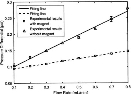
Using the experimental setup shown in Fig. 2-1, we conducted experiments with and without magnet. Speed of the disk was set to be zero in both cases. Silicone oil with known viscosity was first tested as a calibration for the setup. The viscosity of MR fluid with magnet is 3.15 times as large as that of silicone oil. Neither of the fitting line crosses the origin, indicating a constant loss of the setup which may be explained by the curved tubing, increasers and reducers, and the constant offset error of sensors. 0.3 ---- Fitting line ---Fitting line 0.25 Experimental results with magnet A Experimental results i 0.2 without magnet 0.15 0.05 0.1 0.2 0.3 0.4 0.5 0.6 0.7 0.8

Flow Rate (mL/min)

Figure 2-15: Viscosity measurement. Pressure differential (psi) as a function of flow rates (mL/min). Each point corresponds to the mean from three iterations of experiments, with error bars indicating standard deviation. The experiments without magnet was conducted with known viscosity (0.09979 0.00114) Pa-s.

2.4.1 Performance under Poiseuille Flow

Experiments were designed to study the performance with a weak magnetic field

(0.008 T). The mathematical model is detailed in Chapter 2.2. We have built a microchannel network made of a silicon slide, which is laser-cut and sandwiched between two acrylic plates. The flow was driven by pressure gradient using a

syringe pump to control the flow rate.

(a) (b) (c)

(d) (e) (f)

Figure 2-16: Deformation of magnetic chains for different flow rates (Channel width:

0.7 mm, viscosity: 1.78 Pa-s, MR fluid volume fraction: 10%). Flow rates from (a)

to (i): 0.01 mL/min, 0.1 m/min, 1 ml/min, 5 m/min, 10 mL/min, 15 mL/min.

Typical deformations in the channel for different flow rates are displayed in Fig.

2-16 (c). It suggests that the deformation of the magnetic chains is more evident as

flow rates increases and the magnetic chains finally collapse.

Notice that with low flow rate, magnetic chains tend to aggregate in bunches with slight deformation. These chains appear to attach with the vicinity of the walls

of the channel. As the flow rate increases, the chains are more evidently deformed and segregated. It can be observed in Fig. 2-16 (d) that chains start to break at flow rate of 2 mL/min due to higher shear stress, resulting in the detachment from the walls of the channel. After the flow rate at which chains collapse, the channel is filled with uniform particles, the density of which do not change significantly with higher flow rates as shown in Fig. 2-16 (e), (f).

To verify the mathematical model for the magnetic sealing performance at static state, three groups of experiments have been done, and each group of experiments have been repeated for three iterations. Flow rate is controlled by syringe pump, ranging from 0 mUmin to 1.6 mUmin. Pressure differential is acquired by gauge pressure sensors. The experimental results for three different channel widths are shown in Fig. 2-17. 1.4 - -0.5mm 1.2 --

0.5mm

Flow Rate (mL/min)

Figure 2-17: Pressure differential (psi) as a function of flow rate (mUmin), for channel widths from 0.5 mm to 0.9 mm. Each point corresponds to the mean from three iterations of experiments.

As shown in Fig. 2-17, there is a clear pattern shows that the pressure differential will grow as flow rate increases from 0 mL/min; after the peak, if any, it decreases and finally reaches a constant value.

The experimental results are striking. First, the peak point gets more obvious as the width of the channel increases. As for the 0.5 mm channel, the peak can hardly be seen, while the peaks are evident to reach almost 0.8 psi and 1.3 psi for 0.7 mm

channel and 0.9 mm channel respectively. Also, the peak happens at the flow rate of around 0.2 mUmin. It seems that as the channel width increases the peak point will be pushed backward. Furthermore, the slope at 0 mUmin suggests gets steeper as the channel width increases, indicating that the pressure differential grows faster when the channel width is large.

Second, the data suggest that the final value of the pressure differential decreases as the width of the channel gets larger. It appears that it is a non-linear decrease since the difference of the final value of the pressure differential between

0.5 mm channel and 0.7 mm channel is about 0.1 psi, while that between 0.7 mm

channel and 0.9 mm channel is nearly 0.2 psi, almost as twice as the former one. Third, the data indicate that there is a transition between the flow rate of 0.8 mUmin and that of 1.0 mUmin. The intersections of pressure differential under different flow rates happen within the scope of this range. Before this transition, the pressure differential is higher for wider channel width; after this transition, the result is just the opposite.

It can be noticed that, somewhat surprisingly, the peak point lags behind as the channel width gets larger, while the transition point advances. Therefore, as the channel width gets larger and larger, there can be an overlap flow rate range for these two effects. Presumably, these two effects may counteract with each other and finally this interaction may lead to an offset, indicating a flatter and flatter curve when the channel width is large enough.

2.4.2

Performance under Couette Flow

Another experiment was designed to observe the deformation of magnetic brushes under Couette flow. The moving wall was achieved by a disk driven by a motor, of which the rotational speed ranged from 0 rps to 1 rps.

As shown in Fig. 2-17, the left black area of each figure depicts a roughened stationary surface, and the right one depicts a moving wall. As the rotational speed increases, the density of magnetic brushes dramatically decreases with a larger curvature. In addition, the flow rate induced by the rotational disk is reduced by the magnetic brushes; in return, the brushes break when the shear stress is larger than the yield stress.

(a) (b) (c)

Figure 2-18: Deformation of magnetic chains for rotational speed (Channel width:

0.7 mm, viscosity 0.97 Pa-s, MR fluid volume fraction 1%). Rotational speed from

2.5

Dynamic Performance

2.5.1 Hydraulic Performance

Experiments were designed to investigate the sealing performance. The experimental setup is elaborated in Chapter 2.2. Assuming a constant equivalent viscosity of the fluid, the pressure differential increased linearly as a function of flow rate. As the rotational speed increased, the pressure differential went down abruptly from the static state to the dynamic due to the unequally induced Couette flow rate resulted from the asymmetric magnetic field intensity. The flow is modeled as Darcy flow through porous media for one branch, and as Bingham flow for the other. The flow rate induced by the rotational speed of the disk was reduced by the porous media in the branch exposed in stronger magnetic field. This asymmetric induced flow rate accounted for the discrepancy of the pressure differential between the static state and the dynamic. However, as the rotational speed increases, the pressure differential remained nearly stable, indicating that the effectiveness of the porous media was restrained, which could be accounted by the excess of the deformation saturation of magnetic brushes.

0.3 0.25 O.BmUminv C. ~'. 0.2 5 M 0.7mUmin :s 0.2mUmin S01 M.mUmin 0.05 .03~i 0 0 0.2 0.4 0.6 0.8 1 1.2 Rotational Speed (rps)

Figure 2-19: Dynamic sealing performance. Pressure differential (psi) as a function of rotational speed (rps), for flow rates from 0.1 mLJmin to 0.8 mL/min. Each point corresponds to the mean from three iterations of experiments, with error bars indicating standard deviation.

2.5.2

Power Dissipation

A group of experiments were designed to check the hydraulic performance in terms

of power dissipation. As shown in Fig. 2-20, the experimental results suggest that as the rotational speed increases, the power input required gets larger, which is in agreement with the theory that the Couette flow rate induced increases, resulting in a larger power dissipation.

In the experiments, an obvious hysteresis could be noticed for flow rate larger than 0.5 ml/min, resulting in instability for the condition of larger flow rates and

45

Ic

Rotational speed (rps)

Figure 2-20: Power dissipation. Power input (mW) as a function of rotational speed (rps), for flow rates from 0.1 mI~min to 0.8 mUmin. Each point corresponds to the mean from three iterations of experiments.

2.6

Discussions and Evaluations

2.6.1

Dimensional Analysis

The solution variable in our model is the pressure differential between the inlet and outlet AP. The primary variables derives from the geometry, kinematic and the property of the fluid and magnetic field: the diameter of the middle disk D, the width of the channel w, the height of the channel H; viscosity of the fluid with no presence of magnetic field rq; the property of the magnetic field B/pc2 in which B is the magnetic field intensity and p is the magnetic permeability; the average velocity of

' 0.1 mUmin 0"0.2 mUmin

0.3 mnmin

0"0.5

the fluid within the channel U and the rotational velocity of the middle disk (.

By inspection, the dimensionless groups are constructed:

'P _L -=C(D( p , , )(2.29)

B2 _{L hB2 D'D'D}

where AP p h is defined as Mason #2, -- qco as Mason #1, as

B2 _{L hB" D}

dimensionless velocity. The definition of friction factor conforms to the convention, defined as f = AP/ Ipu2 L

2.6.2

Evaluation by Friction Factor and Mason Number

The hydraulic performance of the magnetic sealing, using experimental setup shown in Fig. 2-1, is evaluated by friction factor and Mason number illustrated in Fig. 2-21 and Fig. 2-22 respectively.

Fig. 2-21 suggests that the friction factor experiences a gradually steady growth and dramatically steep increase as Mason #2 decreases. Friction factor, in our experiments, typically indicates the energy loss within the channel, and the Mason #2 directly reflects the pressure differential used to drive Poiseuille flow. The result of this evaluation conforms to the experimental observation that when the pressure differential is low, the density of the magnetic brushes is high with slight deformation, resulting in a higher energy loss.

Fig. 2-22 basically reflects the correlation of the influence of Poiseuille flow and Couette flow. The pattern for Mason #2 and the dimensionless velocity is striking, which can be simply explained by the rotational speed defined in these two dimensionless groups. On the contrary, Mason #2 decreases slightly as Mason #1 varies, suggesting that the influence of Couette flow does not dominate in our experiments. It is considered that the velocity of the disk will induce the maximum

- 3 1 0.75 1 0 c .5 .0 UL 0.25 -1 0 1 0.25 0.8 0.5 0.6 0.4 Mason #1 0.2 1 Mason #2

Figure 2-21: Hydraulic performance evaluated by Friction factor. The ranges of the three dimensionless groups in the figure are scaled down from 0 to 1.

I5 11 2 0.75- 0.8 0.6 0.5 0.4 0 0.2 0.25-, 0 0.8 1 0.5 -0.6 0.5 0.5020.4

Dimensionless velocity 0.2 Mason #1

Figure 2-22: Hydraulic performance evaluated by Mason #2. The ranges of the three dimensionless groups in the figure are scaled down from 0 to 1.

Chapter 3

Design

of

Pumps

Driven

by

Electrorheological Fluid

3.1

Background

Micropumps can generally be classified into two categories: mechanical pumps and non-mechanical pumps. The most common mechanical actuation methods include piezoelectric, bimetallic, thermopneumatic, electrostatic, electromagnetic actuation and shape memory alloy (SMA); the most common non-mechanical actuation methods include magneto-hydrodynamic (MHD), electro-hydrodynamic (EHD), and electro-osmotic actuation.

This chapter introduces a novel actuation method applying electrorheological (ER) fluid. The fluid is driven by the drag force induced by particles subject to dipole-dipole interactions in presence of electric field. In addition, this chapter presents a method of evaluating chamber-pump efficiency in terms of motor efficiency and hydraulic efficiency with mechanical check valve and ER valve.

3.2

Chamber Pumps

3.2.1

Design of Screw-Servo Chamber Pump

A chamber pump driven by servo was designed to evaluate the efficiency of it. As

shown in Fig. 3-1, a servo motor was employed in the setup, providing torque for the screw via a connector. The plunger, driven by the screw, was designed to exert force on the diaphragm. The deformation of the diaphragm forced liquid out of the chamber. Check valve or ER valve orient the fluid. When the diaphragm deformed back, fluid was sucked in.

80 mm _ ,z!' 2 3 4 5 6 7 (a) (b)

Figure 3-1 (a) A picture of the chamber pump. (b) Sectional view of the 3-D model of the chamber pump with one quarter removed. 1: Guider, 2: Plunger, 3: Gasket, 4: Diaphragm, 5: Chamber, 6: Screw, 7: Servo.

Another similar chamber pump is driven by solenoid. The primary advantage, compared to the servo-driven pump, is the higher frequency achieved by solenoid as shown in Fig. 3-2.

Figure 3-2: A picture of the chamber pump driven by solenoid.

3.2.2

Evaluation of motor performance

To measure the efficiency of the motor, a group of experiments were simply designed by measuring the input power and the output power. The input power is the product of current and voltage from the power supply. The output power was measured by a weight and the distance.

As shown in Fig. 3-2, the power input gets larger when the voltage increases. The first 5 seconds shows the servo motor does negative work, while the last 5

seconds positive. The figure suggests that for voltage above 9.0 volts, the power input fluctuates obviously because the output power nearly exceeds the nominal power. In addition, it can be noticed that an apparent overshoot and instability occur during the transition at about 5 seconds. The Chart 3.1 shows the efficiency which is calculated from the results in the last 5 seconds. It indicates that the efficiency peaks at around 6.0 volts, and then drops dramatically.