Author’s Accepted Manuscript
Time-domain seismic modeling in viscoelastic
media
for
full
waveform
inversion
on
heterogeneous computing platforms with OpenCL
Gabriel Fabien-Ouellet, Erwan Gloaguen, Bernard
Giroux
PII:
S0098-3004(16)30781-6
DOI:
http://dx.doi.org/10.1016/j.cageo.2016.12.004
Reference:
CAGEO3882
To appear in:
Computers and Geosciences
Cite this article as: Gabriel Fabien-Ouellet, Erwan Gloaguen and Bernard Giroux,
Time-domain seismic modeling in viscoelastic media for full waveform inversion
on heterogeneous computing platforms with OpenCL,
Computers and
Geosciences,
http://dx.doi.org/10.1016/j.cageo.2016.12.004
This is a PDF file of an unedited manuscript that has been accepted for
publication. As a service to our customers we are providing this early version of
the manuscript. The manuscript will undergo copyediting, typesetting, and
review of the resulting galley proof before it is published in its final citable form.
Please note that during the production process errors may be discovered which
could affect the content, and all legal disclaimers that apply to the journal pertain.
Time-domain seismic modeling in viscoelastic media for full waveform inversion on
1
heterogeneous computing platforms with OpenCL
2
Gabriel Fabien-Ouellet*, Erwan Gloaguen, Bernard Giroux
3
INRS-ETE, 490, Rue de la Couronne, Québec, QC, Canada G1K 9A9 4
*Email address: [email protected]
5
Abstract
6
Full Waveform Inversion (FWI) aims at recovering the elastic parameters of the Earth by matching recordings of the ground motion 7
with the direct solution of the wave equation. Modeling the wave propagation for realistic scenarios is computationally intensive, 8
which limits the applicability of FWI. The current hardware evolution brings increasing parallel computing power that can speed up 9
the computations in FWI. However, to take advantage of the diversity of parallel architectures presently available, new programming 10
approaches are required. In this work, we explore the use of OpenCL to develop a portable code that can take advantage of the 11
many parallel processor architectures now available. We present a program called SeisCL for 2D and 3D viscoelastic FWI in the time 12
domain. The code computes the forward and adjoint wavefields using finite-difference and outputs the gradient of the misfit function 13
given by the adjoint state method. To demonstrate the code portability on different architectures, the performance of SeisCL is tested 14
on three different devices: Intel CPUs, NVidia GPUs and Intel Xeon PHI. Results show that the use of GPUs with OpenCL can speed 15
up the computations by nearly two orders of magnitudes over a single threaded application on the CPU. Although OpenCL allows 16
code portability, we show that some device-specific optimization is still required to get the best performance out of a specific 17
architecture. Using OpenCL in conjunction with MPI allows the domain decomposition of large models on several devices located on 18
different nodes of a cluster. For large enough models, the speedup of the domain decomposition varies quasi-linearly with the 19
number of devices. Finally, we investigate two different approaches to compute the gradient by the adjoint state method and show 20
the significant advantages of using OpenCL for FWI. 21
Keywords
22
OpenCL; GPU; Seismic; Viscoelasticity; Full waveform Inversion; Adjoint state method; 23
1. Introduction
24
In recent years, parallel computing has become ubiquitous due to a conjunction of both hardware and software availability. 25
Manifestations are seen at all scales, from high-performance computing with the use of large clusters, to mobile devices such as 26
smartphones that are built with multicore Central Processing Units (CPU) (Abdullah and Al-Hafidh, 2013). Graphics processing units 27
(GPU) bring this trend to the next level, packing now up to several thousand cores in a single device. Scientific simulations have 28
benefited from this technology through general-purpose processing on graphics processing units and, for certain applications, GPUs 29
can speed up calculation over one or two orders of magnitude over its CPU counterpart. This has caused a surge in the use of GPUs 30
in the scientific community (Nickolls and Dally, 2010, Owens, et al., 2008), with applications ranging from computational biology to 31
large-scale astrophysics. Furthermore, GPUs are increasingly used in large clusters (Zhe, et al., 2004), and now several of the 32
fastest supercomputers on earth integrate GPUs or accelerators (Dongarra, et al., 2015). 33
34
Nevertheless, GPUs are not fit for all kinds of scientific computations (Vuduc, et al., 2010). Potential gains from adopting GPUs 35
should be studied carefully before implementation. In particular, the algorithm should follow the logic of the single-program multiple-36
data (SPMD) programming scheme, i.e. many elements are processed in parallel with the same instructions. In geophysics, and 37
more precisely in the seismic community, GPU computing has been applied most successfully in modeling wave propagation with 38
Finite-Difference Time-Domain (FDTD) schemes. Indeed, the finite-difference method is well suited to GPUs because the solution is 39
obtained by independent computations on a regular grid of elements and follows closely the SPMD model (Micikevicius, 2009). For 40
example, Michéa and Komatitsch (2010) show an acceleration by a factor between 20 to 60 between the single-core implementation 41
of the FDTD elastic wave propagation and a single GPU implementation. Okamoto (2011) shows a 45 times speed-up with a single 42
GPU implementation and presents a multi-GPU implementation that successfully parallelizes the calculation, although with a sub-43
linear scaling. Both Rubio, et al. (2014) and Weiss and Shragge (2013) present multi-GPU FDTD programs for anisotropic elastic 44
wave propagation that shows the same unfavorable scaling behavior. Sharing computation through domain decomposition can be 45
problematic mainly because the memory transfers between GPUs and between nodes are usually too slow compared to the 46
computation on GPUs. GPU computing has also been applied successfully to the spectral element method (Komatitsch, et al., 2010), 47
the discontinuous Galerkin method (Mu, et al., 2013) and reverse time migration (Abdelkhalek, et al., 2009), among others. 48
Nearly all of the seismic modeling codes written for GPUs have been implemented with the CUDA standard (Nvidia, 2007). CUDA 50
allows easy programming on NVidia GPUs; however a CUDA program cannot run on devices other than NVidia GPUs. This can be 51
problematic and is a leap of faith that NVidia devices are and will remain the most efficient devices for seismic modeling. Also, 52
several clusters offer different types of GPU or, at least, a mix of GPU devices. Hence, the choice of CUDA limits the access to the 53
full power of a cluster. On the other hand, OpenCL (Stone, et al., 2010) is an open programming standard capable of using most 54
existing types of processors and is supported by the majority of manufacturers like Intel, AMD and Nvidia. On NVidia’ GPUs, 55
OpenCL performance is comparable to CUDA (Du, et al., 2012). Despite this advantage over CUDA, few published seismic modeling 56
codes use OpenCL: Iturrarán-Viveros and Molero (2013) uses OpenCL in a 2.5D sonic seismic simulation, Kloc and Danek (2013) 57
uses OpenCL for Monte-Carlo full waveform inversion and Molero and Iturrarán-Viveros (2013) perform 2D anisotropic seismic 58
simulations with OpenCL. 59
60
Efficient seismic modeling is more and more needed because of the advent of full waveform inversion (FWI), see Virieux and Operto 61
(2009) for an extensive review. FWI is the process of recovering the Earth (visco)-elastic parameters by directly comparing raw 62
seismic records to the solution of the wave equation (Tarantola, 1984). Its main bottleneck is the numerical resolution of the wave 63
equation that must be repeatedly computed for hundreds if not thousands of shot points for a typical survey. For large-scale multi-64
parameter waveform inversion, FDTD remains the most plausible solution for seismic modeling (Fichtner, 2011). In addition to 65
forward seismic modeling, FWI requires the computation of the misfit gradient. It can be obtained by the adjoint state method 66
(Plessix, 2006), which requires only an additional forward modeling of the residuals. Hence, it is based on the same modeling 67
algorithm and the benefit of a faster FDTD code would be twofold. 68
69
In this study, we investigate the use of OpenCL for modeling wave propagation in the context of time domain FWI. The main 70
objective is to present a scalable, multi-device portable code for the resolution of the 2D and 3D viscoelastic wave equation that can 71
additionally compute the gradient of the objective function used in FWI by the adjoint state method. This paper does not go into 72
specifics about the inversion process, as the gradient calculations calculated by our algorithm is general and can be used in any 73
gradient-based optimization approach. The seismic modeling program, called SeisCL, is available under a GNU General Public 74
License and is distributed over GitHub. The paper is organized in three parts. First, the equations for viscoelastic wave propagation, 75
its finite-difference solution and the adjoint state method for the calculation of the misfit gradient are briefly discussed. In the second 76
part, different algorithmic aspects of the program are presented in detail. The last section presents numerical results performed on 77
clusters with nodes containing three types of processors: Intel CPUs, NVidia GPUs and Intel Xeon PHI. The numerical results show 78
the validation of the code, the computational speedup over a single threaded implementation and the scaling over several nodes. 79
80
2. Theory
81
2.1 Finite difference viscoelastic wave propagation
82
FWI requires the solution of the heterogeneous wave equation. In this study, we consider the wave equation for an isotropic 83
viscoelastic medium in two and three dimensions. We adopt the velocity-stress formulation in which the viscoelastic effects are 84
modeled by generalized standard linear solid (Liu, et al., 1976). The symbols used in this article and their meaning are summarized 85
in table 1. The forward problem in 3D is a set of 9 + 6 simultaneous equations with their boundary conditions: 86 87 (1a) 88 [ (1 + 𝜏𝑝) (1 + 𝛼𝜏𝑝) (1 + 𝜏𝑠) (1 + 𝛼𝜏𝑠)] ( +𝜏𝑠) ( +𝛼𝜏𝑠)( + ) (1b) 89 +𝜏 [( 𝜏𝑝 ( +𝛼𝜏𝑝) 𝜏𝑠 ( +𝛼𝜏𝑠) ) + 𝜏𝑠 ( +𝛼𝜏𝑠)( + ) + ] (1c) 90 | (1d) 91 | , (1e) 92 | , (1f) 93 ( ) , (1g) 94
where Einstein summation convention is used over spatial indices and the Maxwell body indice . Equation 1a comes from 95
Newton’s second law of motion. Equation 1b is the stress-strain relationship for the generalized standard linear solid model with 96
Maxwell bodies, which becomes the generalized Hooke’s law when the attenuation is nil, i.e. when the attenuation levels 𝜏𝑠 and 𝜏𝑝 97
are set to zero. Equation 1c gives the variation of the so-called memory variables. Finally, the last four equations are the boundary 98
conditions, respectively a quiescent past for velocities, stresses and memory variables and a free surface. Those equations are 99
discussed in more details in several papers, see for example Carcione, et al. (1988), Robertsson, et al. (1994) and Blanch, et al. 100
(1995). 101
102
The attenuation of seismic waves is often described by the quality factor, defined as the ratio between the real and imaginary parts of 103
the seismic modulus (O'connell and Budiansky, 1978). In the case of a generalized standard linear solid, it is given by: 104 ( 𝜏 𝜏) +∑ ∑ (2) 105
An arbitrary profile in frequency of the quality factor can be obtained by a least squares minimization over the relaxation times 𝜏
106
and the attenuation level 𝜏. Usually, two or three Maxwell bodies are sufficient to obtain a relatively flat quality factor profile over the 107
frequency band of a typical seismic source (Bohlen, 2002). The two variables involved have different influences on the frequency 108
profile of the quality factor: 𝜏 controls the frequency peak location of the Maxwell body, whereas 𝜏 controls the overall quality
109
factor magnitude. In FWI, an attenuation profile in frequency is usually imposed on the whole domain (Askan, et al., 2007, Bai, et al., 110
2014, Malinowski, et al., 2011) and it is the magnitude of this profile that is sought. For this reason, 𝜏 is taken here as a spatially 111
constant variable that is fixed before inversion, whereas 𝜏 is let to vary spatially and should be updated through inversion. 112
113
To solve numerically equation 1, we use a finite-difference time-domain approach similar to (Levander, 1988, Virieux, 1986). In time, 114
derivatives are approximated by finite-difference of order 2 on a staggered grid, in which velocities are updated at integer time steps 115
and stresses and memory variables are updated at half-time steps in a classic leapfrog fashion. In space, the standard staggered 116
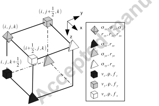
grid is used. An elementary cell of the standard staggered grid is shown in Figure 1, summarizing the location of each seismic 117
variable. The forward + and backward differential operators of order are given by: 118 + ( ) ∑ [ ( + ) ( + 1)] (3a) 119 ( ) ∑ [ ( + 1) ( )] (3b) 120
where is the spatial step and the coefficients are obtained by Holberg’s method (Holberg, 1987) which reduces dispersion 121
compared to the Taylor coefficients. The choice of the forward or backward operator obeys the following simple rule: in the update 122
equations (1a, 1b and 1c) of a variable “a”, to estimate the derivative of a variable “b”, the forward operator is used if variable “b” is 123
located before variable “a” in the elementary cell (Figure 1) along the derivative direction. The backward operator is used otherwise. 124
For example, the update formula for is: 125 + 1 ( + + + ) (4)
The complete set of equations can be obtained with equations 1 and 3 and Figure 1. The reader is referred to the work of Bohlen 126
(2002) for the complete list. 127
128
Finally, to emulate a semi-infinite half-space, artificial reflections caused by the edge of the model must be minimized. For this 129
purpose, two types of absorbing boundaries are implemented: the convolutional perfectly matched layer (CPML) (Roden and 130
Gedney, 2000) as formulated by Komatitsch and Martin (2007) for viscoelastic media and the dissipative layer of (Cerjan, et al., 131
1985). On the top of the model, a free surface condition is implemented by the imaging method of (Levander, 1988). 132
133
134
Figure 1 An elementary cell showing the node location for each seismic variable. 135
136
Table 1 Symbols used in this article 137 Symbol Meaning ( ) Particle velocity ( ) Stress ( ) Source term ( ) Memory variable
⃖ Adjoint variable ( ) Density ( ) P-wave modulus ( ) Shear modulus ( ) Quality factor
𝜏𝑝( ) P-wave attenuation level
𝜏𝑠( ) S-wave attenuation level
𝜏 Stress relaxation time of the lth Maxwell body
Recorded particle velocities
T Recording time
Number of time steps
Cost function
138 139
2.2 Full waveform inversion
140
The goal of full waveform inversion is to estimate the elastic parameters of the Earth based on a finite set of records of the ground 141
motion , in the form of particle velocities or pressure. This is performed by the minimization of a cost function. For example, the 142
conventional least-squares misfit function for particle velocity measurements is: 143 ( 𝜏𝑝 𝜏𝑠) 1 ( ( ) ) ( ( ) ) + ( ( ) ) ( ( ) ) (5) 144
where ( ) is the restriction operator that samples the wavefield at the recorders’ location in space and time. As 3D viscoelastic full 145
waveform inversion may involve billions of model parameters, the cost function is usually minimized with a local gradient-based 146
method. However, due to the sheer size of the problem, the computation of the gradient by finite difference is prohibitive. Lailly 147
(1983) and Tarantola (1984) have shown that the misfit gradient can be obtained by the cross-correlation of the seismic wavefield 148
with the residuals back propagated in time (see Fichtner, et al. (2006) for a more recent development). This method, called the 149
adjoint state method, only requires one additional forward modeling. Based on the method of (Plessix, 2006), it can be shown 150
(Fabien-Ouellet, et al., 2016) that the adjoint state equation for the viscoelastic wave equation of equation 1 is given by: 151 ⃖ + ⃖ (6a) 152 ⃖ + [ (1 + 𝜏𝑝) (1 + 𝛼𝜏𝑝) (1 + 𝛼𝜏(1 + 𝜏𝑠) 𝑠)] ⃖ + (1 + 𝜏𝑠) (1 + 𝛼𝜏𝑠)( ⃖ + ⃖) + ⃖ [ ( +𝜏𝑝) ( +𝛼𝜏𝑝) ( +𝜏𝑠) ( +𝛼𝜏𝑠)] + ( +𝜏𝑠) ( +𝛼𝜏𝑠)(1 + ) (6b) 153
⃖ +𝜏 [( 𝜏𝑝 ( +𝛼𝜏𝑝) 𝜏𝑠 ( +𝛼𝜏𝑠) ) ⃖ + 𝜏𝑠 ( +𝛼𝜏𝑠)( ⃖ + ⃖) + ⃖ ] (6c) 154 ⃖| (6d) 155 ⃖ | , (6e) 156 ⃖ | , (6f) 157 ( ) ⃖ , (6g) 158
with . Comparing equations 1 and 6, we see that both sets of equations are nearly identical, the only difference being the 159
sign of the spatial derivatives and the source terms (the terms involving the misfit function derivative). Hence, the adjoint solution for 160
the viscoelastic wave equation can be computed with the same forward modeling code, with the source term taken as the data 161
residuals reversed in time and with an opposite sign for the spatial derivatives. This allows using the same modeling code for the 162
forward and adjoint problem, with only minor changes to store or recompute the forward and residual wavefields. Once both 163
wavefields are computed, the gradient can be obtained by calculating their scalar product, noted here 〈 〉. The misfit gradient for 164
density, the P-wave modulus, the P-wave attenuation level, the shear modulus and the S-wave attenuation level are given 165 respectively by: 166 167 〈 ⃖ 〉 + 〈 ⃖ 〉 + 〈 ⃖ 〉 (7a) 168 + (7b) 169 𝜏𝑝 𝜏𝑝 + 𝜏𝑝 (7c) 170 + + + (7d) 171 𝜏𝑠 𝜏𝑠 + 𝜏𝑠 𝜏𝑠 + 𝜏𝑠 𝜏𝑠 + 𝜏𝑠 (7e) 172 with 173 ⟨ ⃖ + ⃖ + ⃖ ( + + )⟩, 174 ⟨ ⃖ + ⃖ + ⃖ (1 + 𝜏 )( + + )⟩, 175 ⟨ ⃖ ⟩ + ⟨ ⃖ ⟩ + ⟨ ⃖ ⟩, 176
⟨ ⃖ (( 1) )⟩ + ⟨ ⃖ (( 1) )⟩ 177 + ⟨ ⃖ (( 1) )⟩, 178 ⟨ ⃖ (1 + 𝜏 ) ⟩ +⟨ ⃖ (1 + 𝜏 ) ⟩ 179 +⟨ ⃖ (1 + 𝜏 ) ⟩, 180 ⟨ ⃖ (1 + 𝜏 ) (( 1) )⟩ + ⟨ ⃖ (1 + 𝜏 ) (( 1) )⟩ 181 + ⟨ ⃖ (1 + 𝜏 ) (( 1) )⟩ (7f) 182
where ⃖ ∫ ⃖ , ∑ and is the number of dimensions (2 or 3). Coefficients are given in the
183
appendix. The misfit gradients for the P-wave modulus and the P-wave attenuation level 𝜏𝑝 have the same structure and differ
184
only by the coefficients that weight the scalar products. The same relationship exists between and 𝜏𝑠.
185
In the time domain, the scalar product takes the form: 186
〈 ( ) ( )〉 ∫ ( ) ( ) (8) 187
which is the zero-lag cross-correlation in time of the real-valued functions ( ) and ( ). When discretized in time, it is the sum of 188
the product of each sample. Using Parseval's formula, the last equation can also be expressed in the frequency domain: 189
〈 ( ) ( )〉 ∫ ( ) ( ) (9) 190
where ( ) and ( ) are the Fourier transform of the functions ( ) and ( ) and indicates complex conjugation. The 191
formulation in frequency can be used to perform frequency domain FWI (Pratt and Worthington, 1990) with a time-domain forward 192
modeling code as done by Nihei and Li (2007). The frequency components of the seismic variables can be obtained with the discrete 193
Fourier transform: 194
( ) ∑ ( ) [ ] (10) 195
where is the discrete function in time, A is the discrete function in the Fourier domain, is the time interval, is the frequency 196
interval and is the frequency label. The calculation of a frequency component with the discrete Fourier transform involves the sum 197
of all the time samples weighted by a time varying function given by the complex exponential. In the FDTD scheme, the running sum 198
can be updated at each time step for all or a selected number of frequencies (Furse, 2000). Because FDTD must be oversampled to 199
remain stable (CFL condition), the discrete Fourier transform can be performed at a higher time interval to mitigate its computational 200
cost, e.g. several time steps can be skipped in equation 10, up to the Nyquist frequency of the highest selected frequency. Also, to 201
save memory and reduce computing time, only a handful of frequencies can be used during the inversion (Sirgue and Pratt, 2004). 202
203
Once the gradient is computed, different algorithms can be used to solve the inversion system, from the steepest descent to the full 204
Newton method (Virieux and Operto, 2009). This issue is not the focus of this study. However, all of these local methods need at 205
least the computation of the forward model and the misfit gradient, both of which are the main computational bottlenecks. Hence, a 206
faster forward/adjoint program should benefit all of the local approaches of FWI. 207
208
2.3 Background on heterogeneous computing
209
Heterogeneous computing platforms have become the norm in the high-performance computing industry. Clusters generally include 210
different kinds of processors (Dongarra, et al., 2015): the most common being CPUs, GPUs and Many Integrated Core (MIC), also 211
known as accelerators. Those devices may possess different architecture and usually codes written for one type of device is not 212
compatible with others. Writing a specific code for each type of processor can be tedious and non-productive. One solution is given 213
by OpenCL (Stone, et al., 2010), an open standard cross-platform for parallel programming. OpenCL allows the same code to use 214
one or a combination of processors available on a local machine. This portability is the main strength of OpenCL, especially with the 215
actual trend of massively parallel processors. For the moment, it cannot be used for parallelization on a cluster, but can be used in 216
conjunction with MPI. 217
218
Even though OpenCL allows the same code to be compatible with different devices, the programmer always has to make a choice 219
with the initial design because code optimization can be very different for CPUs, GPUs or MICs architectures. The program 220
presented in this study was written for the GPU architecture, which is arguably the most efficient type of processor available today for 221
finite-difference algorithms. For a good summary of the concepts of GPU computing applied to seismic finite-difference, see (Michéa 222
and Komatitsch, 2010). Essential elements to understand the rest of the article are presented in this section, using the OpenCL 223
nomenclature. 224
A GPU is a device designed to accelerate the creation and manipulation of images, or large matrices, intended primarily for output to 226
a display. It is separated from the CPU (host) and usually does not directly share memory. The set of instructions that can be 227
accomplished on a GPU is different than on the CPU, and classical programming languages cannot be used. A popular application 228
programming interface for GPUs is CUDA (Nvidia, 2007). However, CUDA is a closed standard owned by NVIDIA that can only be 229
used with Nvidia GPUs. It is the main reason why OpenCL was favored over CUDA in this work. 230
231
In order to code efficiently for GPUs, it is important to understand their architecture. The smallest unit of computation is a work item 232
(a thread in CUDA) and is executed by the processing elements (CUDA cores in the NVidia nomenclature). A single device can 233
contain thousands of processing elements that execute the same control flow (instructions) in parallel on different data in the single 234
instruction, multiple thread fashion. The processing elements are part of groups that are called compute units (thread blocks in 235
CUDA). In NVidia devices, the compute units contain 32 consecutive processing elements. In OpenCL, the programmer sends the 236
work items, organized into work groups, to be computed by the processing elements of a compute unit, located in a given device. 237
238
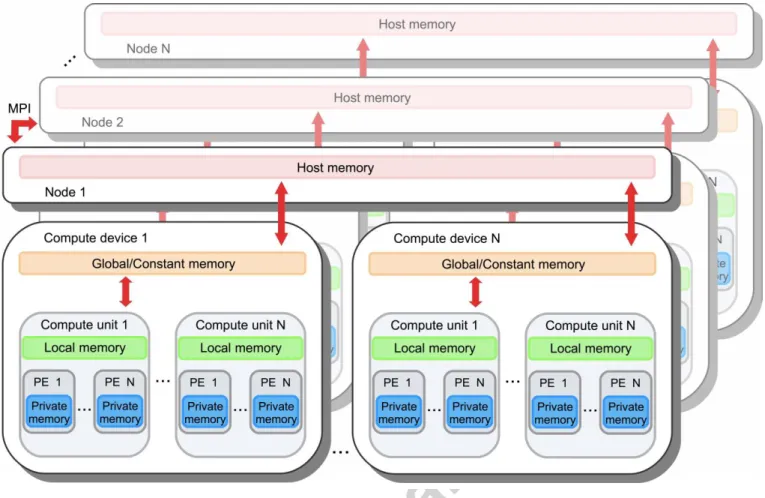
Several levels of memory exist in a GPU. This is schematized in Figure 2, in the context of a GPU cluster. First, each processing 239
element has its own register (private memory), a limited in size but very fast memory. Second, inside each compute unit, threads 240
share a low-latency memory, called the local memory. This memory is small, usually in the order of several kilobytes. The main 241
memory, called global memory, is shared between all processing elements and is the place where the memory needed for the 242
different kernels is located. Usually, this memory is not cached and is very slow compared to the local or private memory. 243
One of the most important aspects of GPU programming is the access to the global memory. Depending on the memory access 244
pattern, read/write operations can be performed in a serial or a parallel fashion by the compute units. Parallel (coalesced) memory 245
access is possible when a number of consecutive work items inside a work group performing the same instructions are accessing 246
consecutive memory addresses. For most NVidia devices, consecutive work items, or what is called a warp, can read 32 floats in a 247
single instruction when memory access is coalesced. With finite-difference codes, the number of instructions performed between the 248
read/write cycles in global memory is fairly low, which means that kernels are bandwidth limited. The memory access pattern is then 249
one of the main areas that should be targeted for optimization. 250
251
Figure 2 OpenCL memory diagram used in conjunction with MPI in the context of a cluster, inspired by (Howes and Munshi, 2014). 252
253
In practice, a program based on OpenCL is organized as follows, regardless of the type of processor used. First, instructions are 254
given to the host to detect the available devices (GPUs, CPUs or accelerators) and connect them in a single computing context. 255
Once the context is established, memory buffers used to transfer data between the host and the devices must be created. Then, the 256
kernels are loaded and compiled for each device. This compilation is performed at runtime. The kernels are pieces of code written in 257
C that contain the instruction to be computed on the devices. After that, the main part of the program can be executed, in which 258
several kernels and memory transfers occur, managed on the host side by a queuing system. Finally, buffers must be released 259
before the end of the program. Several OpenCL instances can be synchronized with the help of MPI, as shown in Figure 2. 260
261
3. Program structure
262
This section describes the implementation of the finite-difference algorithm for viscoelastic modeling and the calculation of the adjoint 263
wavefield in an OpenCL/MPI environment. The program contains many kernels, and its simplified structure is shown in Algorithm 1. 264
This algorithm presents a typical gradient calculation over several seismic shots, on a parallel cluster where each node contains 265
several devices. Its main features are discussed in the following sections. 266
267
Algorithm 1 Pseudo-code for the parallel computation of the gradient with the adjoint state method. 268
Initialize MPI
269
Initialize OpenCL
270
Initialize model grid
271
1. for all groups in MPI do 272
2. for all shots in group do 273
3. for all nodes in group do 274
4. for all devices in node do 275
5. Initialize seismic grid ( ⃖ ⃖ ⃖ ) 276
6. Execute time stepping on shot 277
7. Compute residuals 278
8. Execute time stepping on residuals 279 9. Compute gradient 280 10. end for 281 11. end for 282 12. end for 283 13. end for 284 285
3.1 Node and device parallelism
286
In order to take advantage of large clusters, we use the MPI interface to parallelize computations between the nodes of a cluster. A 287
popular approach to parallelizing finite-difference seismic modeling is domain decomposition (Mattson, et al., 2004). It consists of 288
dividing the model grid into subdomains that can reside on different machines. At each time step, each machine updates its own 289
velocity and stress sub-grids. As the finite-difference update of a variable at a given grid point requires the values of other variables 290
at neighboring grid points (see equations 3 and 4), values defined at grid points on the domain boundary must be transferred 291
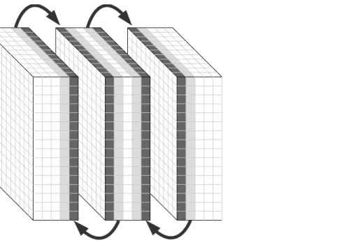
between adjacent domains at each time steps. This is depicted in Figure 3. 292
294
Figure 3 Domain decomposition for three devices for a finite-difference order of 2. Light gray cells are updated inside the device and transferred to the 295
dark gray cells of the adjacent device. 296
297
Fast interconnects are needed for this memory transfer that occurs at each time step, otherwise the scaling behavior can become 298
unfavorable. For example, Bohlen (2002) observes super-linear scaling for up to 350 nodes on a cluster with 450 Mb/s interconnects, 299
but only linear scaling with up to 12 nodes on a cluster with 100 Mb/s interconnects. When using GPUs, not only transfers are 300
needed between nodes, but also between the devices and the host. This dramatically worsens performance. For example, Okamoto 301
(2011) observes a scalability between and . For this reason, we chose to implement two different parallelism schemes in
302
addition to the inherent OpenCL parallelization: domain decomposition and shot parallelization. 303
304
Nodes of a cluster are first divided into different groups: within each group, we perform domain decomposition and each group is 305
assigned a subset of shots. Shot parallelism best corresponds to a task-parallel decomposition, and is illustrated in Algorithm 1 by 306
the loop on all the groups of nodes that starts at line 1, and by the loop on all shots assigned to the groups at line 2. Parallelizing 307
shots does not require communication between nodes and should show a linear scaling. Let’s mention that a typical seismic survey 308
involves hundreds if not thousands of shot points. This should be at least on par with the number of available nodes on large 309
clusters. On the other hand, domain decomposition is required to enable computations for models exceeding the memory capacity of 310
a single device. For this level of parallelism, MPI manages communications between nodes and the OpenCL host thread manages 311
the local devices. The communications managed by MPI and OpenCL are illustrated respectively by the loop on all nodes belonging 312
to the same group starting at line 3 of Algorithm 1 and by the loop on all devices found on the node starting at line 4. 313
314
To further mitigate the communication time required in domain decomposition, the seismic updates are divided between grid points 315
on the domain boundary that needs to be transferred and interior grid points that are only needed locally. This is described in 316
Algorithm 2. The grid points on the boundary are first updated, which allows overlapping the communication and the computation of 317
the remaining grid points, i.e. lines 3 and 4 and lines 7 and 8 of Algorithm 2 are performed simultaneously for devices supporting 318
overlapped communications. This is allowed in OpenCL by having two different queues for each device: one for buffer 319
communication and the other for kernel calls. 320
321
Algorithm 2 Pseudo code showing the overlapping computation and memory transfer for domain decomposition. 322
1. while t < Nt
323
2. Call kernel_updatev on domain boundary 324
3. Transfer in boundary of devices, nodes 325
4. Call kernel_updatev on domain interior 326
5. Store ( ) in seismo at t 327
6. Call kernel_updates on domain boundary 328
7. Transfer in boundary of devices, nodes
329
8. Call kernel_updates on domain interior 330 9. Increment t 331 10. end while 332 333
3.2 GPU kernels
334The main elements of the kernels used to update stresses and velocities are shown in Algorithm 3. For better readability, the 335
algorithm is simplified and does not include viscoelastic computations or CPML corrections. Note that the “for” loops in this pseudo-336
code are implicitly computed by OpenCL. The most important features of this algorithm are steps 3 and 4, where seismic variables 337
needed in the computation of the spatial derivatives are loaded from the global memory to the local memory. As the computation of 338
the spatial gradient of adjacent grid elements repeatedly uses the same grid points, this saves numerous reads from global memory. 339
To be effective, those reads must be coalesced. This is achieved by setting the local working size in the z dimension, which is the 340
fast dimension of the arrays, to a multiple of 32 for NVidias’ GPUs. Hence, seismic variables are updated in blocks of 32 in the z 341
dimension. In the x and y dimensions, the size of the local working size does not impact coalesced memory reading. They are set 342
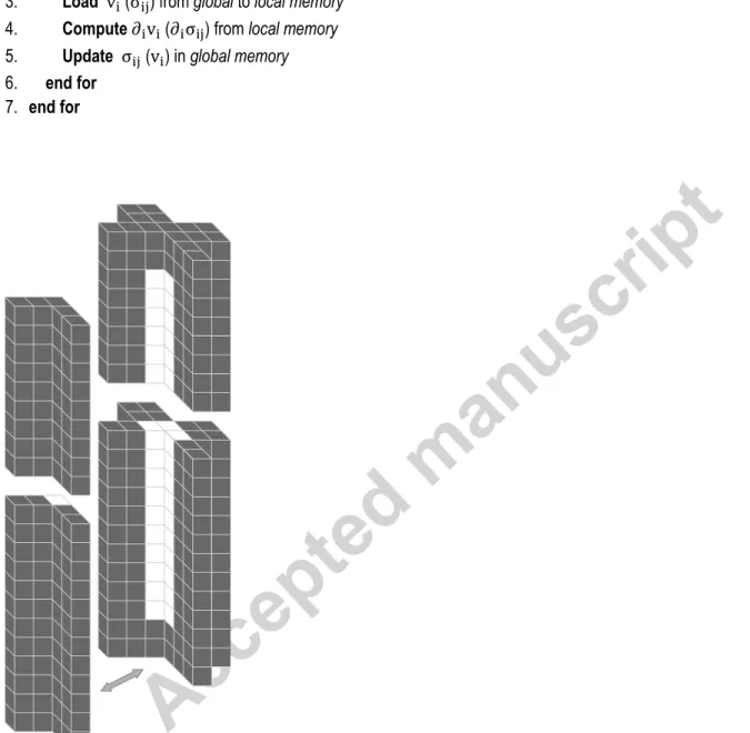
equal to a magnitude that allows all the seismic variables needed in the update to fit in the local memory. This is illustrated in Figure 343
4. 344
345
Algorithm 3 Pseudo code for the seismic update kernels showing how local memory is used. 346
1. for all local_domains in global_domain do 347
2. for all grid point in local_domain do 348
3. Load ( ) from global to local memory
349
4. Compute ( ) from local memory 350
5. Update ( ) in global memory 351 6. end for 352 7. end for 353 354 355 356
Figure 4 Exploded view of the local memory containing a seismic variable during update (equations 1a and 1b), for the 2nd order scheme. White cells
357
are cells being updated and gray cells are loaded into local memory only to update white cells. 358
359
3.3 Misfit gradient computation
360
The cross-correlation of the direct and residual fields requires both fields to be computed at the same time step (see equation 8). 361
This is challenging because forward computations are performed from time zero, whereas adjoint computations are performed from 362
final time. Several strategies can be employed to achieve this task (see (Dussaud, et al., 2008, Nguyen and McMechan, 2015) for 363
comparisons between methods). 364
1. When propagating the direct field, the whole grid for the particle velocities and stresses at each time step or a subset of the 365
time steps can be saved into memory. When the residual field is propagated from final time, the direct field is read from 366
memory for all grid points and the scalar product is evaluated iteratively, time step per time step. 367
2. In the so-called the backpropagation scheme (Clapp, 2008, Yang, et al., 2014), only the outside boundary of the grid that is 368
not in the absorbing layer is saved at each time step. The direct field is recovered during the residual propagation by 369
propagating back in time the direct field from the final state, injecting the saved wavefield on the outside boundary at each 370
time step. As both the forward and adjoint wavefields are available at the same time step, the scalar products can be 371
computed directly with equation 8. 372
3. A selected number of frequencies of the direct and residual field can be stored. This is performed by applying the discrete 373
Fourier transform incrementally at each time step (equations 9 and 10), as done by (Sirgue, et al., 2008). The scalar product 374
is evaluated at the end of the adjoint modeling in the frequency domain with equation 9. An alternative way of computing the 375
chosen frequencies (Furse, 2000) seems to be advantageous over the discrete Fourier transform, but has not been tested 376
in this study. 377
4. In the optimal checkpointing method proposed by (Griewank, 1992, Griewank and Walther, 2000), and applied by (Symes, 378
2007), the whole forward wavefield is stored for a limited number of time steps or checkpoints. To perform the scalar 379
product, the forward wavefield is recomputed for each time step during the backpropagation of the residuals from the 380
nearest checkpoint. For a fixed number of checkpoints, an optimal distribution that minimizes the number of forward 381
wavefield that has to be recomputed can be determined. For this optimal distribution, the number of checkpoints and the 382
number of recomputed time steps evolve logarithmically with the number of total time steps. Further improvements of the 383
method have been proposed by (Anderson, et al., 2012) and by (Komatitsch, et al., 2016) in the viscoelastic case. 384
385
The first option is usually impractical, as it requires a huge amount of memory even for problems of modest size. In 3D, it requires on 386
the order of ( ) elements to be stored, which becomes quickly intractable. Let’s mention that the use of compression and 387
subsampling can be used to mitigate these high memory requirements (Boehm, et al., 2016, Sun and Fu, 2013). The 388
backpropagation scheme requires far less memory, on the order ( ) in 3D, but doubles the computation task for the direct 389
field. Also, it is not applicable in the viscoelastic case. Indeed, in order to back-propagate the wavefield, the time must be reversed 390
and, doing so, the memory variable differential equation (equation 1c) becomes unstable. Hence, when dealing with 391
viscoelasticity, the frequency scheme and the optimal checkpointing scheme are the only viable options. The memory requirement of 392
the frequency scheme grows with the number of computed frequencies on the order of ( ). However, as is common in FWI, 393
only a selected number of frequencies can be used (Virieux and Operto, 2009). The optimal checkpointing method requires 394
( ) where is the number of checkpoints. Because of the logarithmic relationship between the number of time steps, the 395
number of checkpoints and the number of additional computations, the required memory should stay tractable. For example, for 10 396
000 time steps, with only 30 buffers, the computing cost of this option is 3.4 times that of the forward modeling. In this work, we 397
implemented the backpropagation scheme for elastic propagation and the frequency scheme using the discrete Fourier transform for 398
both elastic and viscoelastic propagation. The implementation of the optimal checkpointing scheme or the hybrid 399
backpropagation/checkpointing scheme of (Yang, et al., 2016) is left for future work. 400
401
The gradient computation involving the backpropagation of the direct field is illustrated in Algorithm 4. At each time step of the direct 402
field propagation, the wavefield value at grid points on the outer edge of the model is stored. Because of the limited memory capacity 403
of GPUs, this memory is transferred to the host. As mentioned before, this communication can be overlapped with other 404
computations with the use of a second queue for communication. After obtaining the residuals, the residual wavefield is propagated 405
forward in time using the same kernel as the direct wavefield. The back-propagation of the direct wavefield is calculated using the 406
same kernel, the only difference being the sign of the time step . Also, at each time step, the stored wavefield on the 407
model edges is injected back. With this scheme, both the residual and the direct fields are available at each time step and can be 408
multiplied to perform on the fly the scalar products needed to compute the gradient. 409
Algorithm 4 Pseudo code for the backpropagation scheme. 410
1. while t < Nt
411
2. Call kernel_updatev 412
3. Store in boundary of model 413
4. Call kernel_updates 414
5. Store in boundary of model 415 6. Increment t 416 7. end while 417 8. Calculate residuals 418 9. while t < Nt 419 10. Call kernel_updatev on ⃖ 420
11. Inject in boundary of model 421
12. Call kernel_updates on ⃖ 422
13. Inject in boundary of model 423 14. Compute gradient 424 15. Increment t 425 16. end while 426 427
The frequency scheme is illustrated in Algorithm 5. It first involves computing the direct wavefield and its discrete Fourier transform 428
on the fly at each time step, for each desired frequency (equation 10). Afterward, the residual wavefield is obtained in exactly the 429
same fashion. At the end, the scalar product needed for the gradients can be computed with the selected frequencies. 430
431
Algorithm 5 Pseudo code for the frequency scheme. 432
1. while t < Nt
433
2. Call kernel_updatev for 434
3. Call kernel_updates for
435
4. Call DFT for for freqs 436 5. Increment t 437 6. end while 438 7. Compute residuals 439 8. while t < Nt 440
9. Call kernel_updatev for ⃖ 441
10. Call kernel_updates for ⃖ 442
11. Call DFT for ⃖ ⃖ for freqs 443 12. Increment t 444 13. end while 445 14. Compute gradients 446 447
4. Results and discussion
448
This section shows several numerical results obtained with SeisCL. The following tests were chosen to verify the performance of 449
OpenCL in the context of FWI on heterogeneous clusters containing three different types of processors: Intel CPUs, Intel Xeon PHI 450
(MIC) and NVidia GPUs. 451
4.1 Modeling validation
452
In order to test the accuracy of our forward/adjoint modeling algorithm, two synthetic cases are presented. First, the finite-difference 453
solution of the viscoelastic wave equation is compared to the analytic solution. The analytic solution for the viscoelastic wave 454
propagation of a point source derived by Pilant (2012) is used here in the form given by Gosselin-Cliche and Giroux (2014) for a 455
quality factor profile corresponding to a single Maxwell body. The source is a Ricker wavelet with a center frequency of 40 Hz, 456
oriented in the z direction. The viscoelastic model is homogeneous with 𝑝=3500 m/s, 𝑠=2000 m/s, =2000 m/s with a single
457
Maxwell body. We tested 4 attenuation levels 𝜏𝑝 𝜏𝑠 { 1 }, i.e. { 1 } at the center frequency of 458
40 Hz. Using a finite-difference stencil of order 4, a 6 m (8.33 points per wavelength) spatial discretization is used to avoid numerical 459
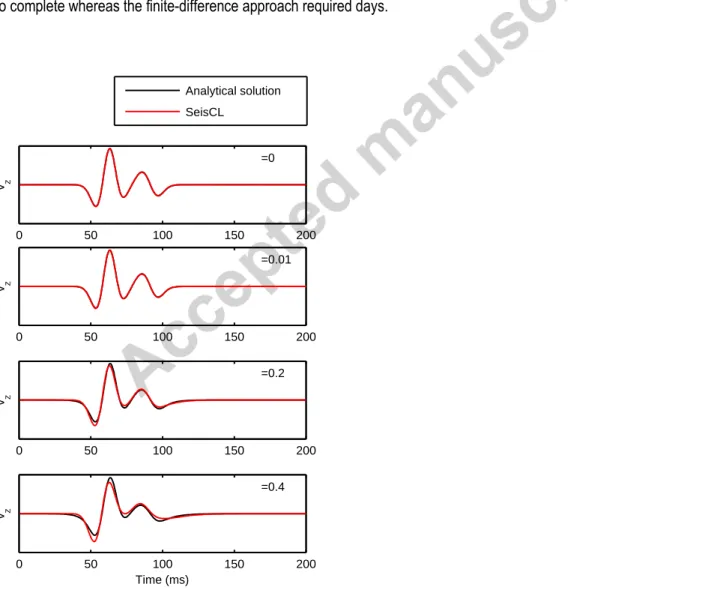
dispersion with a 0.5 ms time step for numerical stability. Figure 5 shows the comparison between the analytic solution and the 460
solution obtained with SeisCL. The traces represent the particle velocities in the z direction for an offset of 132 m in the z direction. 461
For the elastic case (𝜏=0), the analytical solution is perfectly recovered by SeisCL. Using higher attenuation levels does, however, 462
introduce some errors in the solution. This error increases with 𝜏 and for an attenuation level of 0.4, the discrepancy becomes 463
obvious for the offset used herein. It is, however, the expected drawback of using an explicit time domain solution and similar time-464
domain algorithms show the same behavior, see (Gosselin-Cliche and Giroux, 2014). Also, for reasonable attenuation levels, the 465
errors appear negligible and will not impact FWI results much. Accuracy could become an issue for very high attenuating media and 466
long propagation distances. 467
468
The second test aims at validating the misfit gradient output of SeisCL. For this test, a synthetic 2D cross-well tomographic survey is 469
simulated, where a model perturbation between two wells is to be imaged. The well separation is 250 m and the source and receiver 470
spacing are respectively 60 m and 12 m (Figure 5). Circular perturbations of a 60 m radius for the five viscoelastic parameters were 471
considered at five different locations. The same homogeneous model as the first experiment is used with 𝜏 =0.2 and with 472
perturbations of 5 % of the constant value. Because significant crosstalk can exist between parameters, especially between the 473
velocities and the viscous parameters (Kamei and Pratt, 2013), we computed the gradient for one type of perturbation at a time. For 474
example, the P-wave velocity gradient is computed with constant models for all other parameters other than 𝑝. This eliminates any 475
crosstalk between parameters and allows a better appraisal of the match between the gradient update and the given perturbations. 476
Note that because the goal of the experiment is to test the validity of the approach, geological plausibility was not considered. As no 477
analytical solution exists for the gradient, the adjoint state gradient was compared to the gradient computed by finite-difference. The 478
finite-difference solution was obtained by perturbing each parameter of the grid sequentially by 2%, for all the grid position between 479
the two wells. The adjoint state gradient was computed with the frequency scheme using all frequencies of the discrete Fourier 480
transform between 0 and 125 Hz. 481
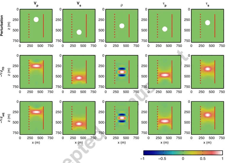
The results of this second experiment are shown in Figure 6. In this figure, each column represents a different perturbed parameter. 483
The first row shows the perturbation, the second the steepest descent direction (minus the misfit gradient) obtained by finite-484
difference and the third the steepest descent direction given by the adjoint state model. Note that the gradients were normalized in 485
this figure. As can be visually appraised, an excellent agreement is obtained between both methods, for all parameters. Although the 486
inversion has not been performed here, it should converge to the right solution in the five different cases, the update correction being 487
already in the right direction. This is expected considering the small value of the perturbation used in this experiment; the inverse 488
problem is more or less linear in such circumstances. The good agreement between the finite-difference and the adjoint state 489
gradients shows that the latter could be used in any gradient-based inversion approach. However, the adjoint approach is orders of 490
magnitude faster than the finite-difference approach: the first grows proportionally to the number of frequencies (see next section) 491
while the second grows linearly with the number of parameters. For this particular experiment, the adjoint approach required minutes 492
to complete whereas the finite-difference approach required days. 493
494
495
Figure 5 Comparison between the analytical solution and SeisCL results for different attenuation levels, from the elastic case ( =0) to strong
496 viscoelasticity ( =0.4). 497 0 50 100 150 200 t=0 v z Analytical solution SeisCL 0 50 100 150 200 t=0.01 v z 0 50 100 150 200 t=0.2 v z 0 50 100 150 200 t=0.4 v z Time (ms)
498 499 500
501
Figure 6 A cross-well experiment to test the validity of the misfit gradient. The red triangles represent the sources position and the red dots the 502
receiver positions. Each column represents a different parameter. The first row shows the location of the perturbation, the second row represents the 503
opposite of the misfit gradient obtained by finite-difference and the third row represents the opposite of the misfit gradient obtained by the adjoint 504 state method. 505 506
4.2 Performance comparison
507The effort required to program with the OpenCL standard would be vain without a significant gain in the computing performance. In 508
the following, several tests are presented to measure the performance of SeisCL. As a measure, one can compute the speedup, 509
defined here as: 510
𝑠
𝑠 (11)
Different baselines are used depending on the test. In order to show the OpenCL compatibility of different devices, all tests are 512
performed on three types of processors: Intel CPUs, Intel Xeon PHI (MIC) and NVidia GPUs. Unless stated otherwise, the CPU 513
device consists of 2 Intel Xeon E5-2680 v2 processors with 10 cores each at a frequency of 2.8 GHz and with 25 MB of cache. The 514
GPU is an NVidia Tesla K40 with 2880 cores and 12 GB of memory, and the MIC is an Intel Xeon Phi 5110P. 515
516 517
4.2.1- Speedup using SeisCL over a single threaded CPU implementation 518
As a baseline, SOFI2D and SOFI3D, the 2D and 3D implementations of Bohlen (2002) are used with a single core. This baseline can 519
be compared to SeisCL as both codes use the same algorithm. It is also representative of the speed that can be achieved for a 520
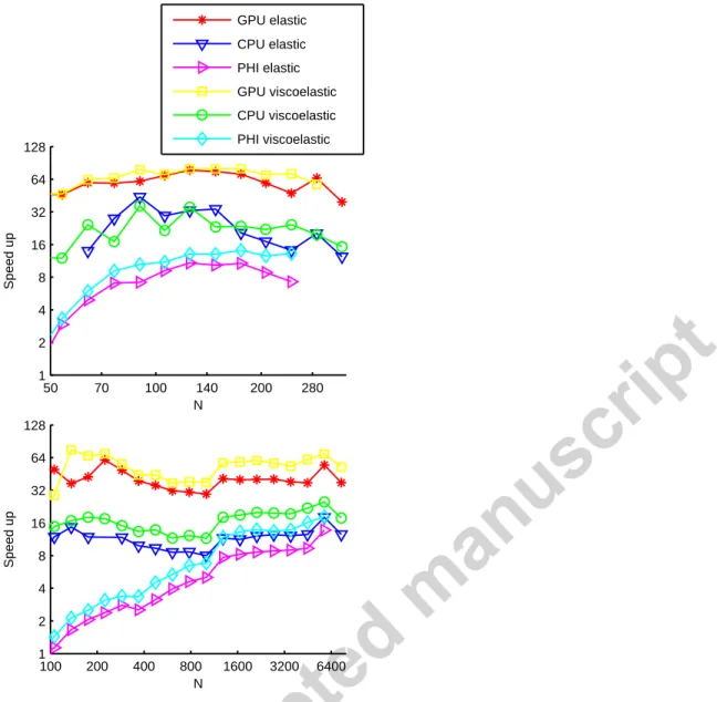
FDTD code written in C, arguably one of the fastest high level languages for the CPU. In Figure 7, the speedup is measured as a 521
function of the model size for the 3D and 2D cases, where the model size is a cube and a square respectively with edges of N grid 522
points. The speed-up varies significantly with the model size. The highest speedups are attained with the GPU, which ranges 523
between 50 to more than 80 in 3D and between 30 and 75 in 2D. Significant speedups are also obtained with CPUs, as high as 35 524
times faster. This is higher than the number of cores (20) available. We make the hypothesis that this is caused by a better cache 525
usage of the OpenCL implementation, i.e. usage of local memory increases significantly the cache hits during computation compared 526
to the C implementation of Bohlen (2002). The 2D implementation seems less impacted by this phenomenon and speedups are in a 527
more normal range, between 11 and 25. We also noted that the time stepping computation can be very slow in the first several 528
hundred time steps for the C implementation. This is the source of the strong variations in speedups observed in Figure 7. Finally, 529
the Xeon Phi speedups are disappointing compared to their theoretical computing capacity. However, SeisCL has been optimized for 530
GPUs, not for the Xeon Phi. Even if we have not tested it, it is possible that with small modifications of the code, improved 531
performance could be attained. This shows, however, the limits of device portability with OpenCL: code optimization is paramount to 532
achieve high performances and this optimization can be quite different for different devices. 533
534
Figure 7 Speedup of SeisCL over a single threaded CPU implementation for different model sizes in 3D (top) and 2D (bottom), for different processor 535
types. 536
537
4.2.2- Performance of the gradient calculation 538
The next test aims at assessing the performance of the two different gradient schemes. For this experiment, the baseline is the time 539
required to perform one forward modeling run, without the gradient calculations. The computing times are measured for the 540
backpropagation scheme and the frequency scheme, for model sizes of 100x100x100 and 1000x1000 grid nodes in 3D and 2D 541
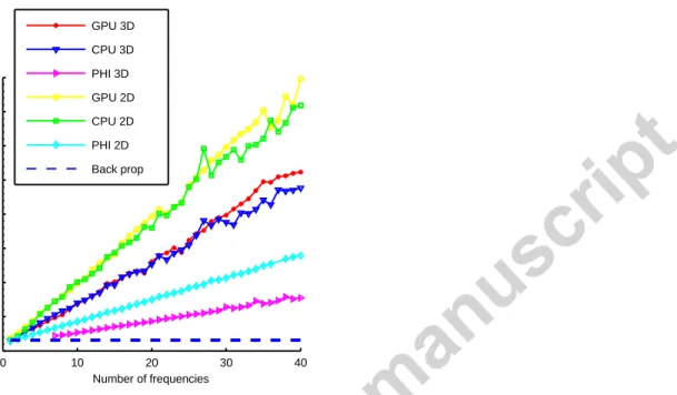
respectively. The results are shown in Figure 8. For the frequency scheme, the computing time increases linearly with the number of 542
frequencies. The cost rises faster in 3D than in 2D, which can be explained by the higher number of variables needed to be 543
transformed in 3D. Surprisingly, the computation time for the Xeon PHI seems to increase much slower than for the CPU or the GPU. 544
It is to be noticed that for testing purposes, the discrete Fourier transform was computed at every time step. However, significant 545 50 70 100 140 200 280 1 2 4 8 16 32 64 128 S p e e d u p N 100 200 400 800 1600 3200 6400 1 2 4 8 16 32 64 128 S p e e d u p N GPU elastic CPU elastic PHI elastic GPU viscoelastic CPU viscoelastic PHI viscoelastic
savings could be achieved if it was computed near the Nyquist frequency. Nevertheless, this test shows that the cost of computing 546
the discrete Fourier transform during time stepping is not trivial but remains tractable. Finally, the backpropagation scheme has a 547
cost that is roughly 3 times the cost of a single forward modeling for all devices. Hence, in the elastic case, the backpropagation 548
scheme outperforms the frequency scheme no matter the number of frequencies. It also has the added benefit of containing all 549
frequencies. 550
551
Figure 8 Ratio of the computing time between the forward modeling and the adjoint modeling in the frequency scheme for an increasing number of 552
frequencies. The dashed line denotes the back-propagation scheme for all devices. 553
554 555
4.2.3- Measure of the cost of using higher order finite-difference stencils on different devices 556
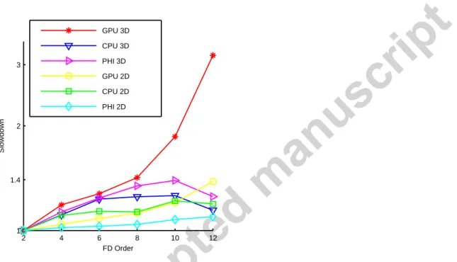
The baseline for this test is the computation time of the 2nd order stencil for each device. The slowdown is used here as a measure,
557
i.e. the inverse of the speedup. The same spatial and temporal step lengths were used for each order. As can be seen in Figure 9, 558
for all three types of device, the slowdown is quite low and does not exceed 1.5 for the highest order of 12 considered here, except 559
for the GPU in 3D where it exceeds 3 for an order of 12. Note that up to the 8th order, the GPU performance is comparable to the
560
other device types. The higher cost for the GPU in 3D for orders 10 and 12 is caused by the limited amount of local memory. Indeed, 561
for those orders, the amount of local memory required to compute the derivative of a single variable exceeds the device capacity. In 562
those circumstances, SeisCL turns off the usage of local memory and uses global memory directly. The abrupt slowdown is manifest 563
of the importance of using local memory. The reason why higher order stencils do not affect significantly the computing time of 564
SeisCL is that it is bandwidth limited: access to the memory takes more time than the actual computations. As memory access is 565 0 10 20 30 40 0 10 20 30 40 50 60 70 80 S lo w d o w n Number of frequencies GPU 3D CPU 3D PHI 3D GPU 2D CPU 2D PHI 2D Back prop
locally shared, the higher number of reads required for higher finite-difference order does not increase significantly. The impact on 566
computation at each time step is thus marginal. In most cases, the advantages of using higher orders outweigh the computational 567
costs, because it allows reducing the grid size. For example, using a 6th order over a 2nd order stencil allows reducing the grid point
568
per wavelength from around 22 to 3, i.e. it reduces the number of grid elements by a factor of 400 in 3D. However, in some 569
situations, for instance in the presence of a free surface, topography or strong material discontinuities, higher order stencils introduce 570
inaccuracies (Bohlen and Saenger, 2006, Kristek, et al., 2002, Robertsson, 1996). Hence, the choice of the order should be 571
evaluated on a case-by-case basis. 572
573
574
Figure 9 Slowdown of the computation using higher finite-difference order compared to the 2nd order for different devices.
575 576
4.2.4- Tests on heterogeneous clusters 577
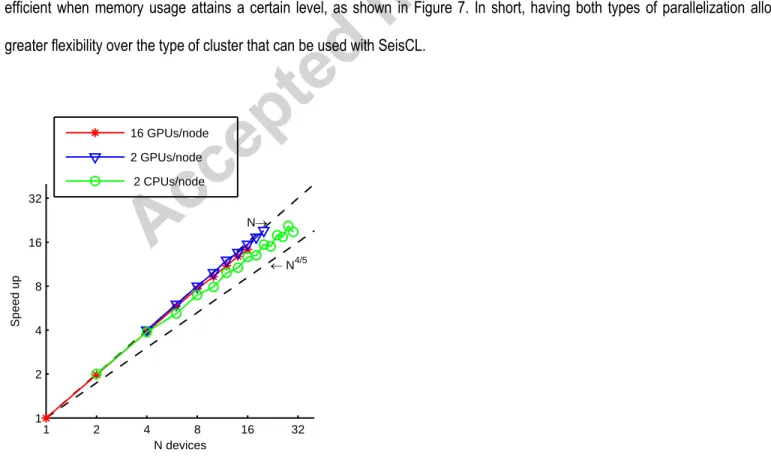
To evaluate the scalability of our code over large clusters, a strong scaling test was performed. Here, strong scaling refers to the 578
variation of the computational time for a model of fixed sized for an increasing number of processors. The following results were 579
obtained for a grid size of 96x96x9000 elements and an increasing number of devices for the domain decomposition. This test was 580
performed on two different clusters: Helios of Laval University, Canada and Guillimin from McGill University, Canada. The Helios 581
nodes contain 8 NVidia K80 GPUs (16 devices). This cluster was used to test strong scaling for GPUs on a single node of a cluster, 582
which does not involve MPI. Two types of nodes were used on Guillimin: nodes containing two Intel Xeon X5650 with 6 cores each at 583 2 4 6 8 10 12 1 1.4 2 3 S lo w d o w n FD Order GPU 3D CPU 3D PHI 3D GPU 2D CPU 2D PHI 2D
2.66 GHz and 12 MB of cache and nodes containing 2 NVidia K20 GPUs in addition to the same two Xeon CPUs. This cluster was 584
used to test strong scaling across several nodes, which requires MPI communication. 585
586
Results are shown in Figure 10. The best scaling behavior is shown by the nodes on Guillimin with two GPUs, which is very nearly 587
linear over the tested number of devices (blue triangles on Figure 10). Surprisingly, the scaling is slightly worse for many devices 588
located on the same node (Helios nodes, red stars in Figure 10). We interpret this result as being caused by the increasing burden 589
on the processor when a higher number of GPUs must be scheduled on the same nodes: at some point, the CPU becomes too slow 590
to keep all GPUs busy. Compared to Guillimin nodes using CPUs, Guillimin nodes using GPUs also scale better. Still, the CPU 591
scaling remains quite favorable and is higher than N4/5. Those results are better than the results reported by Okamoto (2011), Rubio,
592
et al. (2014), Weiss and Shragge (2013). We explain this favorable behavior by the separate computation of grid elements inside and 593
outside of the communication zone in our code. 594
The strong scaling tests show that for large models that fit only on multiple nodes and devices, SeisCL can efficiently parallelize the 595
computation domains with a minimal performance cost. Still, parallelization over shots should be favored when models fit in the 596
memory of a single device because no fast interconnects are needed in this situation, and because SeisCL is somewhat more 597
efficient when memory usage attains a certain level, as shown in Figure 7. In short, having both types of parallelization allows a 598
greater flexibility over the type of cluster that can be used with SeisCL. 599
600
601
Figure 10 Strong scaling tests for a grid size of 96x96x1000. Red corresponds to results from Helios. Green and blue to Guillimin. 602 1 2 4 8 16 32 1 2 4 8 16 32 N® ¬ N4/5 S p e e d u p N devices 16 GPUs/node 2 GPUs/node 2 CPUs/node
603
5. Conclusion
604
In this article, we presented a program called SeisCL for viscoelastic FWI on heterogeneous clusters. The algorithm solves the 605
viscoelastic wave equation by the Finite-Difference Time-Domain approach and uses the adjoint state method to output the gradient 606
of the misfit function. Two approaches were implemented for the gradient computation by the adjoint method: the backpropagation 607
approach and the frequency approach. The backpropagation approach was shown to be the most efficient in the elastic case, having 608
roughly the cost of 3 forward computations. It is, however, not applicable when viscoelasticity is introduced. The frequency approach 609
has an acceptable cost when a small number of frequencies is selected, but becomes quite prohibitive when all frequencies are 610
needed. Future work should focus on the implementation of the optimal checkpointing strategy, which is applicable to both elastic 611
and viscoelastic FWI and strikes a balance between computational costs and memory usage. 612
It was shown that using OpenCL speeds up the computations compared to a single-threaded implementation and allows the usage 613
of different processor architectures. To highlight the code portability, three types of processors were tested: Intel CPUs, Nvidia 614
GPUs and Intel Xeon PHI. The best performances were achieved with the GPUs: a speedup of nearly two orders of magnitude over 615
the single-threaded code was attained. On the other hand, code optimization was shown to be suboptimal on the Xeon PHI, which 616
shows that some efforts must still be spent on device-specific optimization. For the GPU, memory usage was the main area of code 617
optimization. In particular, the use of OpenCL local memory is paramount and coalesced access to global memory must be 618
embedded in the algorithm. 619
When using domain decomposition across devices and nodes of a cluster, overlapping communications and computations allowed 620
hiding the cost of memory transfers. Domain decomposition parallelization was shown to be nearly linear on clusters with fast 621
interconnects using different kinds of processors. Hence, SeisCL can be used to compute the misfit gradient efficiently for large 3D 622
models on a cluster. Furthermore, the task-parallel scheme of distributing shots allows flexibility when the speed of interconnects 623
between the nodes limits the computational gain. Together, both parallelization schemes allow a more efficient usage of large cluster 624
resources. 625
In summary, the very good performance of SeisCL on heterogeneous clusters containing different processor architectures, 626
particularly GPUs, is very promising to speed up full waveform inversion. Presently, the most efficient devices for SeisCL are GPUs, 627
but this can change in the future. The open nature and the flexibility of OpenCL will most probably allow SeisCL to use new hardware 628
developments. SeisCL is distributed with an open license over Github. 629
630
Apppendix A
631
This section lists the misfit gradient coefficients. First, some constants are defined: 632 𝛼 ∑ 𝜏 + 𝜏 (A-1) 633 ( ( +𝜏𝑝) ( +𝛼𝜏𝑝) ( 1) ( +𝜏𝑠) ( +𝛼𝜏𝑠)) (A-2) 634 ( 𝜏𝑝 ( +𝛼𝜏𝑝) ( 1) 𝜏𝑠 ( +𝛼𝜏𝑠)) (A-3) 635 636
The misfit gradient coefficients are given by: 637 ( +𝜏𝑝) ( +𝛼𝜏𝑝) (A-4) 638 𝜏𝑝 ( +𝛼𝜏𝑝) (A-5) 639 ( +𝛼𝜏𝑠) ( +𝜏𝑠) (A-6) 640 ( + ) ( +𝜏𝑠) ( +𝛼𝜏𝑠) (A-7) 641 ( +𝛼𝜏𝑠) ( +𝜏𝑠) (A-8) 642 ( +𝛼𝜏𝑠) 𝜏𝑠 (A-9) 643 ( + ) 𝜏𝑠 ( +𝛼𝜏𝑠) (A-10) 644 ( +𝛼𝜏𝑠) 𝜏𝑠 (A-11) 645 𝜏𝑝 (1 𝛼) ( +𝛼𝜏𝑝) (A-12) 646 𝜏𝑝 ( +𝛼𝜏 𝑝) (A-13) 647 𝜏𝑠 ( 𝛼) ( +𝜏𝑠) (A-14) 648
𝜏𝑠 ( + ) (1 𝛼)( +𝛼𝜏 𝑠) (A-15) 649 𝜏𝑠 ( 𝛼) ( +𝜏 𝑠) (A-16) 650 𝜏𝑠 𝜏𝑠 (A-17) 651 𝜏𝑠 ( + )( +𝛼𝜏 𝑠) (A-18) 652 𝜏𝑠 𝜏𝑠 (A-19) 653
Acknowledgements
654This work was funded by a Vanier Canada Graduate Scholarship and supported by the Canada Chair in geological and geophysical 655
data assimilation for stochastic geological modeling. 656
657 658
References
659
Abdelkhalek, R., Calandra, H., Coulaud, O., Roman, J. and Latu, G., 2009, Fast seismic modeling and Reverse Time Migration on a 660
GPU cluster, p. 36-43, 10.1109/hpcsim.2009.5192786. 661
Abdullah, D. and Al-Hafidh, M. M., 2013, Developing Parallel Application on Multi-core Mobile Phone: Editorial Preface, v. 4, no. 11. 662
Anderson, J. E., Tan, L. and Wang, D., 2012, Time-reversal checkpointing methods for RTM and FWI: Geophysics, v. 77, no. 4, p. 663
S93-S103, 10.1190/geo2011-0114.1. 664
Askan, A., Akcelik, V., Bielak, J. and Ghattas, O., 2007, Full Waveform Inversion for Seismic Velocity and Anelastic Losses in 665
Heterogeneous Structures: Bulletin of the Seismological Society of America, v. 97, no. 6, p. 1990-2008, 10.1785/0120070079. 666
Bai, J., Yingst, D., Bloor, R. and Leveille, J., 2014, Viscoacoustic waveform inversion of velocity structures in the time domain: 667
Geophysics, v. 79, no. 3, p. R103-R119, 10.1190/geo2013-0030.1. 668
Blanch, J. O., Robertsson, J. O. A. and Symes, W. W., 1995, Modeling of a constantQ: Methodology and algorithm for an efficient 669
and optimally inexpensive viscoelastic technique: Geophysics, v. 60, no. 1, p. 176-184, 10.1190/1.1443744. 670
Boehm, C., Hanzich, M., de la Puente, J. and Fichtner, A., 2016, Wavefield compression for adjoint methods in full-waveform 671
inversion: Geophysics, v. 81, no. 6, p. R385-R397, 10.1190/geo2015-0653.1. 672
Bohlen, T., 2002, Parallel 3-D viscoelastic finite difference seismic modelling: Computers & Geosciences, v. 28, no. 8, p. 887-899, 673
10.1016/s0098-3004(02)00006-7. 674
Bohlen, T. and Saenger, E. H., 2006, Accuracy of heterogeneous staggered-grid finite-difference modeling of Rayleigh waves: 675
Geophysics, v. 71, no. 4, p. T109-T115, 10.1190/1.2213051. 676
Carcione, J. M., Kosloff, D. and Kosloff, R., 1988, Viscoacoustic wave propagation simulation in the earth: Geophysics, v. 53, no. 6, 677
p. 769-777, 10.1190/1.1442512. 678
Cerjan, C., Kosloff, D., Kosloff, R. and Reshef, M., 1985, A nonreflecting boundary condition for discrete acoustic and elastic wave 679
equations: Geophysics, v. 50, no. 4, p. 705-708, 10.1190/1.1441945. 680
Clapp, R. G., 2008, Reverse time migration: saving the boundaries, Technical Report SEP-136, Stanford Exploration Project, p. 137. 681
Dongarra, J. J., Meuer, H. W. and Strohmaier, E., 2015, Top500 supercomputer sites, http://www.top500.org/ (Accessed on 682
01/12/2015) 683