Device modelling of a field emission displays

Device Modelling of Field Emission Displays

by

Pei-Ning Wang

Submitted to the Department of Electrical Engineering and Computer Science

in partial fulfillment of the requirements for the degrees of

Master of Engineering in Electrical Engineering and Computer Science

and

Bachelor of Science in Electrical Science and Engineering

at the

MASSACHUSETTS INSTITUTE OF TECHNOLOGY

May 1996

@ Pei-Ning Wang, MCMXCVI. All rights reserved.

The author hereby grants to MIT permission to reproduce and distribute publicly

paper and electronic copies of this thesis document in whole or in part, and to grant

others the right to do so.

Author...

...

....

...

...

Department of Ele- ical Engineeriig and Computer" Science

May 28, 1996

Certified by ...

Tayo Akinwande

Associate Professor

Thesis Supervisor

Accepted by...

Chairman, Departmental

\

Frtederic

R. Morgenthaler

ommittee on Graduate Students

MASSACHUSETTS INSTI'FUTE

OF TECHNOLOGY

JUN

11

1996

Device Modelling of Field Emission Displays

by

Pei-Ning Wang

Submitted to the Department of Electrical Engineering and Computer Science on May 28, 1996, in partial fulfillment of the

requirements for the degrees of

Master of Engineering in Electrical Engineering and Computer Science and

Bachelor of Science in Electrical Science and Engineering

Abstract

In recent times, field emission displays (FEDs) have generated a lot of interest because they feature the advantages of both CRT and the prevalent flat panel display technologies. The fast pace of current developments in field emission arrays (FEAs) demonstrate a need for efficient device simulation software. The simulation should be capable of calculating electron trajectories from the emitter to the screen and current density distributions on the phosphor screen. It should also have the ability to simulate the distribution of electrons for a lone emitter, as well as for an entire field emitter array (FEA). In addition, the software should be robust, so that various cathode geometries may be implemented; and modular, so that many cathode array elements may be easily simulated together. This thesis describes such a tool for calculating the electron trajectories of field emission cathodes of various geometries.

Thesis Supervisor: Tayo Akinwande Title: Associate Professor

Acknowledgments

I would like to thank everyone who have given me so much of their time and support during these last few months. Largely, I would like to thank my parents for their encouragement and generosity which has made my life at MIT so much easier and carefree.

Next, I would like to thank Professor Akinwande for his guidance and sensitivity. He is a marvelous advisor, both at a academic level and a personal level. I hope that many other students will take advantage of the opportunity to benefit from him, as I have.

And also I must thank Dr. John Gilbert for his insight and expertise. John has met with Professor Akinwande and myself at practically every meeting. Thanks for your time and advice! Your suggestions have directed my thesis, and put me on the right track toward graduating.

In addition, I would like to thank Professor Senturia and his research group for sharing a few of the machines in their laboratory. Thank you, I could not run my simulations without your help.

And a special thanks goes to Julian Verdejo, whose assurances has kept me smiling through these last days at MIT.

Contents

2.1 Prevalent Flat-Panel Technologies 2.2 Emissive Technologies ...

2.2.1 Field Emission Displays . . 2.2.2 Description of FEAs . . .. 2.2.3 Problems with FEAs . ... 2.3 Existing Device Analysis Programs

3 Overview of Virtual-FED: the FED Device Sir 3.1 General Description ...

3.2 Virtual-FED Implementation Details ... 3.2.1 Special Constructs ...

3.2.2 Octree Field Estimation ...

3.2.3 Trajectory Convergence Implementation 3.2.4 Monte Carlo Implentation ...

3.3 Limitations and Requirements . ... 3.4 Virtual-FED Usage ... nulEitor 23 . . . . 25 . . . . . 28 . . . . 28 . . . . 34 . . . . . 34 . . . . 35 . . . . . 36 . . . . 36

4 Virtual-FED Simulation Results

4.1 Sample Trajectory Evaluations ...

41 42

4.1.1 Electron Self-Focusing ... 45

4.1.2 The Effects of Gate Voltages ... 48

4.1.3 Distribution Effects ... 51

4.1.4 The Effects of Initial Electron Energy . ... 57

4.2 Comparison of Virtual-FED Results with Analytical Expressions ... 61

5 Conclusions and Recommendations 63 5.1 Recommendations for Future Work ... 65

5.1.1 Integration with MEMCAD ... 65

5.1.2 Trajectory Test Programs ... 65

5.2 Conclusions ... ... ... 67 A trajectory.h 71 B trajectory.h 77 C octree.h 103 D octree.m 107 E initial.m 131 F sample main.c 133

List of Figures

2-1 Color LCD Cross-Section . . . . 2-2 A single emitter in a field emission display . . 2-3 Major Types of Field Emitter Arrays (FEAs)

3-1 3-2 3-3 3-4 3-5 3-6 3-7 3-8 3-9 3-10 3-11 4-1 4-2 4-3 4-4 4-5 4-6 4-7 4-8 4-9

Virtual-FED Processes: Flow Chart ...

Top Octree Box ...

Box Data Structure ... Support Structures for Box ... Octree Data-Structures ...

Diagram of Simplified Octree Structure .. Trajectory Data-Structures ...

Diagram of Trajectory Structure ... Semi-Circular Cone Emitter ...

Virtual-FED: Structures User Must Initialize Virtual-FED Sample Code ...

Range of theta: VA = 2000V, VG = 100V, E = 0.1eV . .

Self Focusing: Distribution of Electrons Positions . . . . Self Focusing: Energy Distribution ...

Gate and Anode Voltages: Distribution of Electron . . . Gate and Anode Voltages: Energy Distribution . . . . . Uniform Probability Density Function f() . . . .

Gaussian Probability Density Function fo(O), oe = 0.88 . Gaussian Probability Density Function fo(O), ao = 0.2 . Distribution Effects: Distribution of Electron I . . . . .

. . . . 26 . . . . 29 . . . . 30 . . . . 31 . . . . 32 . . . . 32 . . . . 33 . . . . 34 . . . . 35 S . . . . . 38 *. . . . . 40 . . . . . 43 . . . . . 46 ... . 47 . . . . . 49 . . . . . 50 . . . . . 52 . . . . . 52 . . . . . 53 . . . . . 54

4-10 Distribution Effects: Distribution of Electron II . ... 55

4-11 Distribution Effects: Energy Distribution . ... 56

4-12 Effects of Initial Electron Energy: Distribution of Electrons . ... 59

4-13 Effects of Initial Electron Energy: Energy Distribution . ... 60

5-1 IFE-FEA Structure with Focus Electrodes at Gate Level . ... 66

List of Tables

2.1 Comparison of Flat-Panel Display Technologies . ... 14

2.2 AMLCD Luminous Efficiency ... .15

4.1 Parameter Values for Virtual-FED Test Cases . ... 45

4.2 Test Parameters: Self-Focusing Examples . ... 45

4.3 Test Parameters: Effect of Gate Voltage . ... .. 48

4.4 Test Parameters: Effect of Initial Velocity Distributions . ... 53

Chapter 1

Introduction

In recent years, flat-panel displays have found broad acceptance and application in the areas of portable information systems, such as lap-top computers used for in-field data-acquisitioning and record keeping. In addition, military and avionic groups have expressed interest in flat-panel technologies, with emphasis on developing interfaces for intelligent human-machines [1]. The commercial applications of flat-panels are endless, ranging from products such as personal notebooks to large-screen, HDTV systems. This growing demand for flat-panel technologies has demonstrated a need for developing a flat display technology with high resolution and high brightness, while still maintaining low power consumption and cost.

Although conventional CRTs have exceptional brightness and resolution characteristics, they are unsuited to the needs of portable systems due to bulkiness and weight constraints. Prevalent flat-panel technologies are lightweight and thin solutions, with tradeoffs in pic-ture quality and power consumption. However, present day advances in integrated circuit fabrication technology have allowed Field Emission Displays (FEDs) to emerge as an alter-native flat-panel display technology. This latest technology functions essentially as a flat panel CRT, and hence, brings the best qualities of the CRT together with the portability of flat-panel displays.

These desired qualities motivate FED researchers to advance at lighting speed. In order for the science of FEDs to continue at its current rapid pace, designers need efficient simulation models for FED environments. Thus far, FED development has been restrained by the lack of computer simulation tools. CAD tools are necessary to keep development

time and costs at a minimum.

1.1

Problem Statement

Despite the fast pace of development in FED technology, FED developers are still unsure about future directions in the field. There are a number of questions which need to be answered before the technology can reach its full potential. FED researchers would like to know the effects of specific design choices on FED performance before an FED is physically implemented. Their questions include:

* What are optimal gate, screen, and focus electrode (if present) operating volt-ages?

* Given device dimensions and voltage parameters, what is the current density distribution (spot size) on the phosphor screen?

* What parameters are necessary to produce a reliable and reproduceable device? * How does emitter geometry affect current uniformity?

* How closely should field emitters be spaced in an FED?

* To what extent do focusing electrodes help narrow the electron beam? * How far vertically from the emitter should the focusing electrode be spaced? * How far can the distance between the emitter cathode and the screen be

ex-tended with the usage of various focusing electrodes?

If a suitable electron trajectory simulation program were available, it could have the ca-pability of predicting accurate solutions to these questions for FED developers. To date, there are no available CAD tools which adequately model field emitter array (FEA) device performance. And prior to the start of this work, there appeared to be no leads for future designs.

The benefit of having such a CAD tool is that it would bring FED development time and costs to a minimum. It would be able to propel FED technology forward by allowing the simulation of novel devices, without the costs and hassle of physical implementation. In addition, a FED device simulator could allow FED designers to find the parameters to optimize an implementation. In order for a FED design to be an optimal design, it must demonstrate a high proficiency within four key attributes [2]:

* Feasibility of large size cathode with uniform electron emission and high manu-facturing yield

* Feasiblility of full color device with brightness, resolution and high luminous efficiency at moderate anode voltage.

* Acceptable driving voltages. * Long life.

A CAD tool, which calculates electron trajectories to predict spot size upon the screen, could effectively determine the first three characteristics for an optimal FED device. The key feature of a CAD utility is to estimate the current density distribution of a single emitter on screen of the display, taking into account the variations of emission current. After the calculation of the current distribution from a single emitter, the solution may be replicated at various positions on the FEA and superimposed to give an overall current density distribution for the screen. With these qualities, the CAD software would be a useful analytical and predictive tool for estimating the relationship between device spot size and the physical design parameters, such as the optimal spacing between the cathode and screen and the cone to cone spacings in FEAs.

Currently, the FED industry needs computer simulation tools equivalent to the design tools which have revolutionized other engineering fields, such as IC design and fabrication. VLSI CAD utilites including CADENCETM and MentorGraphicsTM have produced rad-ical changes in the IC hardware industry by allowing product development times to decrease dramatically; thereby, lowering costs and increasing innovation. FED technology could ben-efit immensely with a complementary device simulation program, parallel to those of the VLSI industry.

1.2

Research Objectives

The research objective of this paper is to design Virtual-FED, a CAD utility which is suitable for modelling FEAs. The intended purpose of the program is to predict the current density distribution, along the monitor screen, as a function of gate and anode potentials and arbitrary emitter spacings. Using Virtual-FED software, FED designers will be able to predict the brightness, spot size, and their uniformity across the screen.

The Virtual-FED utility is similar to existing FEA simulating software. However, in addition to the features described by other methods, the discussed simulation predicts

a current density distribution on the screen and introduces a monte carlo scheme which models the effects from variations of emission current and estimate actual current den-sity/uniformity at the screen. The following is a listing of the essential elements of the Virtual-FED software.

* Calculate electric field (boundary element method)

* Compute current density on emitter tip using the Fowler-Nordheim Theory * Simulate the electron trajectory

* Calculate the current density distribution on the screen

* Use monte carlo technique to account for non-normal electron emission * Correlate the calculated current density distribution with actual data

The unique contribution of this CAD design is that it calculates current density dis-tributions, and uses a monte carlo technique for determining electron emissions which are non-normal to the surface of the emitter tip. The monte carlo scheme allows for predictions of actual experimental distributions; this capability can be extremely useful. For exam-ple, such a tool could be used to predict the minimum tip radius required for a particular brightness or uniformity. It could also be used to estimate the minimum spacings between emitters for a given spot size.

Other advantages of this proposed implementation are that it enables the design of novel FEA structures and displays, and the utility will be integrated with MEMCAD, which provides a fast and efficient means for calculating electric fields.

1.3

Overview

The next chapter, Chapter 2, presents a brief background of current flat-panel technologies. First, a description of the various display types is given in order to form a comparative benchmark with FED displays. Then, the advantages and disadvantages of emissive displays are discussed; and the physical nature of FED environments is introduced. Finally, previous work involving computer analysis to model current distributions on the FED monitor screen is presented.

A complete description of the Virtual-FED simulation program is given in Chapter 3. An overview of the simulation procedure for calculating electron trajectories and electron

energy distributions at the screen is given in the first section. The next section focuses on implementation details, such as the special constructs. Then, the limitations and require-ments for using Virtual-FED are outlined. Lastly, the procedure for using the program is presented.

Several test cases, generated with the Virtual-FED utility, are presented in Chapter 4. The results of these examples form general conclusions about issues, such as (i) the anode operating voltage, or self-focusing, (ii) gate operating voltage, (iii) current distribution, and (iv) the initial energy of the electron. After each of these points are discussed, concerns about the simulator accuracy and practicality are addressed.

The final chapter contains a discussion of the performance of Virtual-FED and sugges-tions for future work. Possible future extensions of this thesis work are also introduced.

Chapter 2

Background

Recent popularity of portable information systems has led to a need for developing low cost and low power technologies for flat panel displays. Current flat-panel display technology offers a wide variety of implementations: passive and active-matrix liquid-crystal displays (LCDs), electroluminescent displays (ELDs), plasma display panels (PDPs), and vacuum fluorescent displays (VFDs), and so on. Each of these implementations has its own advan-tages and disadvanadvan-tages (refer to [3] for a detailed overview). However, for a typical lap-top computer, the display itself embodies 40 - 50% the cost of the system, and consumes ap-proximately 50% of the power in the entire system. In fact, none of the current flat-panel technologies satisfy the requirement for portable information systems; which demand low power, high luminous efficiency, high contrast, high information content and full color. They must at the same time have small volume and be lightweigth. Table 2.1 summarizes the governing attributes of popular flat-panel technologies.

The most dominant display technology is the cathode ray tube (CRT). It is efficient in power however bulky and unportable. An ideal case would feature (1) the high efficiency of CRTs, (2) the portability of flat panel displays, and (3) low cost in manufacturing. FED technology has the potential for providing all of these features, since it is essentially a flat CRT.

To date, the LCD display is the most advanced of the plat-panel displays under develop-ment. In recent years, improvements in manufacturing technologies have allowed LCDs to gain wide acceptance. This flat-panel architecture has dominated the market for portable computers, lap-tops, and other portable computing systems. In addition, LCDs are

becom-Table 2.1: Comparison of Flat-Panel Display Technologies

Shadow Mask Liquid

Electro-

Vacuum

Plasma

Cathode Ray Crystal luminescent Fluorescent Display

Tube Display Display Display

Power Consumption 200W 100W 40 - 50W 60W 60 - 80W

Contrast Ratio Excellent Medium Good Good Good

(with filter) (with filter) (with filter) (with filter)

Viewing Angle Excellent Poor Good Excellent Excellent

Luminance 350cd/m2 350cd/m 2 100cd/m2 70cd/m2 70cd/m2

(with filter) (with filter)

Color Best Full Green or Full Full

yellow

Resolution Excellent Excellent Excellent Satisfactory Satisfactory

High Ambient Light Good Excellent Satisfactory Poor Satisfactory

Readability (with filter) (with filter) (with filter)

Frame Rate 60Hz 60Hz 60Hz 60Hz 60Hz

Pixel Matrix 2048 x 2048 1024 x 1024 864 x 1024 400 x 640 2048 x 2048

Temperature Excellent Poor Satisfactory Satisfactory Satisfactory

Resistance

Humidity Resistance Satisfactory Poor Satisfactory Satisfactory Satisfactory Shock and Vibration Satisfactory Excellent Excellent Satisfactory Excellent Resistance

Price Very low High Moderate Low Moderate

ing incorporated into products, such as flat screen and projection entertainment systems.

2.1

Prevalent Flat-Panel Technologies

Liquid-crystal display (LCD), the prevalent flat panel technology, works essentially as an addressable light valve, composed of a polarizable liquid-crystal material sandwiched between two sheets of glass (See Figure 2-1). Along the surface of the glass sheets are layers of transparent conducting material. An electric field can be induced in the liquid-crystal by applying a voltage across the conductors; this field rotates the orientation of molecules in the liquid-crystal. Light generated by the backlight/diffuser is sent through a pre-polarizer and then this filter. The intensity of light at the screen is determined by the rotation angle of the liquid-crystal molecules. When the backlight passes through the filters, it loses intensity. Overall, in a full color LCD, only about 5% of light from the backlight actually

Table 2.2: AMLCD Luminous Efficiency Theoretical Actual Backlight 50lumen/watt Diffuser 30% First Polarizer 50% 43 - 45% Aperture Ratio of TFT/LC 50 - 50% Color Filters 33% 25%

Small Losses (Absorption/Reflections) 90%

Exit Polarizer 87 - 89%

Luminous Efficiency (excluding Diffuser) • 5%

Luminous Efficiency (including Diffuser) < 2.5%

Luminous Efficiency of AMLCD 1 llumen/watt

Image

I

Exit

nAigpment Conduc tor Ac tiue

ITnsparent

I

~ ~ ~

~

~

~

cnmccxcc~cc~cxo~r-siiw

~

~

BACKLIGHT/IFFUSER

reaches the screen. This is summarized in Table 2.2.

Although LCDs are easily addressable and inexpensive to produce, they do have many shortcomings: (1) the requirement of a uniform and controlled light source, (2) restrictions in the dynamic range of color for each pixel, (3) the loss of at least one-half of the total light through the basic polarization process, (4) slow refresh rates due to the slow response time of the liquid-crystal, (5) a strong variation of light intensity at different viewing angles, (7) sensitivity to temperature and pressure, and (8) filters must be matched with the color spectrum of the light source [3].

2.2

Emissive Technologies

LCDs have other disadvantages which are non-existent with emissive display implementa-tions such as CRTs and FEDs. CRTs produce light extremely efficiently through cathodo-lumminescence - the process by which light is produced from an electron striking a phosphor. The advantage of cathodolumminescence is that the quality and intensity of light may be controlled and also the light is unpolarized and may be viewed over a wide angle without variation in intensity, color purity, or contrast. Several advantages of cathodoluminescence are listed from Henry Gray in his article 'The field-emitter display' [3].

* High Iuminous efficiency * High brightness

* High dynamic range in brightness * Full color

* Outstanding color purity * Wide viewing angle * High spatial resolution

* Designable persistence (to prevent flickering, yet allow a fast refresh) * "Simple" manufacturing processes

2.2.1

Field Emission Displays

The primary problem with the CRT display is that it is requires much volume and weight. These qualities are mainly attributed to the bulkiness of the cathode ray tube. The proposed

Photons

Stf

Indium

Phosphors

Extraction Electcode 2 mm

Gate

Resistive,0Em•

•i

Inulitoz

Glass

Figure 2-2: A single emitter in a field emission display

solution is to create FEDs which combine the advantages of cathodoluminescence with the desirable volume and weight of current flat panel displays.

The FEDs offers a more elegant implementation of the CRT, by replacing the single cathode ray tube with a two dimensional array of minute cathode emitters, known as field emitter arrays (FEAs). FEAs have the following properties [3],

* Individual pixel can be targeted on or off

* Has built in sub-pixel redundancy - if one elementary cells fail, others still work * Can be batch fabricated

* Has high spatial resolution * Capable of high current density * Is temperature insensitive

* Can be made extremely thin or flat

2.2.2

Description of FEAs

A single emitter in a field emitter array (FEA) acts as a miniature electron gun (See Figure

2-2). When a sufficiently large voltage is applied between the emitter and the gate, by means

of the extraction electrodes, electrons tunnel out of the emitter. The electrons accelerate

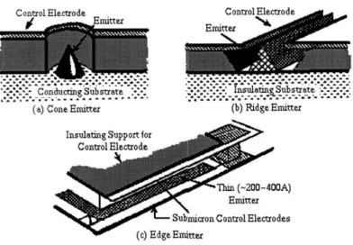
Electrons tunnel from the emitter when a large electric field on the order of 109V/m

C ontrol Electrode

(a) Cone Emitter (b) Ridge Emitter

%J -. U. -5 =...L .

Figure 2-3: Major Types of Field Emitter Arrays (FEAs)

The rate of change of electrons across the area of the emitter may be described by the Fowler-Nordheim equation for current density [4],

J

=

(y-where t2(y) = 1.1, v(y) = 0.95 - y2, A = 1.54 x 10-6, B = 6.87 x 107, and y = 3.79 x

10- 4E1/2/0. Increasing the total current density from an emitter increases the brightness of the corresponding pixel [5]. This fact enables easy adjustment over the resolution and contrast of the image.

Since the electric field is naturally strongest around the tip of a sharp object, shaping a cathode emitter with the geometry of a sharp object, such as a cone, greatly reduces the potential necessary to make electrons arc from the emitter. With a pointed design, operational voltage ranges from 100V-300V, rather than 1000V-30000V [6, 1976]. The major designs of FEAs are shown in Figure 2-3.

2.2.3 Problems with FEAs

The main challenges confronting FED development are (i) development of spacers between the screen and gate substrate, and (ii) issues of uniformity, reliability, and stability. Spacers must be strong enough to sustain an evacuated cavity and thin enough so that they do not interfere with the current density distribution on the screen. In addition, current FEDs use low voltage phosphors which have poor efficiency, about 51umen/Watt, as compared to CRTs which use high voltage phosphors with an efficiency of 25lumen/Watt. Current

FED technology does not allow for the usage of higher voltage phosphors because of spacer breakdown at shorter distances. Also, if higher voltages were used, a trade-off occurs between resolution and efficiency, since increasing the voltage level requires an increase in vacuum gap [7]. And thus, an increase in spot size follows. One solution is to add a focusing electrode aperture within the vacuum region itself. Designing such a structure would require CAD tools, which have yet to be developed. Discussed issues with FEAs are listed in a nutshell:

* Necessity for strong, long-lived spacers

* Current FEDs, using low voltage phosphors, are inefficient (5 Lumen/Watt) * Trade-off between decreasing spot-size, i.e. increasing resolution, and decreasing

luminous efficiency. This can be avoided by the use of higher screen voltages with the appropriate spacers and electron focusing optics.

* Need for focusing electrodes

* No appropriate CAD tools exist for modelling FEDs and FEAs.

2.3

Existing Device Analysis Programs

As mentioned in Chapter 1, to date, there are no available CAD tools which accurately model FEA performance.

In their paper Modelling of a Field Emision Display Using the Adaptive Scheme Method, Kyung C. Choi and Nagyoung Chang describe an adaptive scheme method which calculate the trajectories of electrons when a low voltage is applied to the anode of a cone-shaped emitter [8] (See Figure 2-2). Characteristics of the electron contact position with the phos-phor screen were discussed, as well as the effects concerning varying the emitter tip radius, etc. However, the paper does not mention the capability to calculate current density dis-tributions on the phosphor screen. Without this feature, their utility is not a practical predictor of spot size or resolution.

W. Dawson Kesling and Charles Hunt describe a technique for simulating the perfor-mance of field emitters in FEDs, combining both finite element and finite difference analysis [9]. Their program is similar to this work, using emission currents, along the cathode surface, which are calculated from the Fowler-Nordheim equation, and trajectories are calculated using a fourth-order finite difference scheme. However, it has several limitations. At far

distances from the cathode, trajectories are extrapolated using the exact solution for elec-trons in a uniform field. This shows that the difference scheme is not self adjusting, i.e. it does not self compensate for the changing strengths of the fields. In addition, they have assumed a cylindrically symmetric field about the emitter environment, so their program cannot explore outcomes based upon asymmetrical irregularities on the cone's surface.

In their paper Electron-beam induced deposition for fabrication of vacuum field emitter

devices, the team of Weber, Rudolph, Kretz, and Koops relate a Monte-Carlo simulation

program. The simulation is used to model the scattering of the primary electrons in an emitter tip, in order to calculate the spatial distribution of leftover energy at the tip [10]. Although, the program is capable of calculating beam energy, the current, and the effects of material properties at the tip. It does not go on to calculate actual electron trajectories and the current density distribution along the surface of the screen.

Fedirko, Belova, and Makhov describe a physical and mathematical simulation model for calculating the effectiveness of beam control optimization [11]. Their work takes ad-vantage of the cylindrical symmetry for a cone-shaped FED device; however, this restricts the program to only symmetrically shaped devices. This confinement makes their program unsuitable for the calculation, of spot size and resolution, for all FED device geometries

Munro, Zhu, Rouse, Liu present a 3D finite difference program, that calculates electron trajectories using the fourth-order Runge-Kutta algorithm in their paper entitled Computer

Simulation of Vacuum Microlectronic Components [12]. The program uses special equations

at the interfaces between the electrodes and the free space regions. The potential values, calculated from the equations, are stored in a three-dimensional grid point system. This program is extremely similar to the proposed Virtual-FED implementation. Their paper does not mention whether the finite difference method, that they are using, is self adjusting to compensate for highly varying fields. In addition, they do not describe any special methods, involve in the implementation of their three-dimensional grid lookup table. Hence, one cannot conclude from their paper, if they have a fast and efficient simulation program for modelling FED devices.

In summary, existing FED device simulation programs have many design flaws. For example, most of the programs use finite differece methods; however none of them mention the capability to self adapt in step sizes. Without the ability to self adjust, they shall need to scale geometries much bigger or change anode sizing in order to provide computationally

reasonable results. In addition, most recent FED device simulators describe their programs to utilize cylindrical symmetry the cone-shaped emitters. These implementations will not be able to support any FED devices which are asymmetrical about the z-axis.

It is necessary to design a program that can start from a geomentry of fine granuarity, that self adjusts into coarser environment. In addition, it should be able to compute entire FEAs.

Chapter 3

Overview of Virtual-FED: the

FED Device Simulator

The FED device simulator, Virtual-FED, models field emission devices, particularly the field emitter display. The simulation package is intended to be used to explore field emission design as well as to help develop and analyze experiments to illuminate the underlying factors that describe field emission from manufactuable material surfaces.

Virtual-FED is intended for generalized device analysis and design. It is currently built to be included as a module of an existing software system, MEMCAD. MEMCAD is de-signed to model arbitrary three-dimensional device structures, which helps build structures from mask and process information. It already has existing modules for solving 3D elec-trostatics, structural mechanics, and coupled-electromechanics. In future implementations, the Virtual-FED will use the MEMCAD system to construct models of arbitrary field emit-ter geometry and calculate electric fields throughout the device. However, in this thesis an analytical field solution is used. Electron emission current density at the field emitter tip are calculated by assuming the electrons are emitted normal to the surface. This is refined to take into account non-zero tangential electron energy. The Monte-Carlo and other statistical techniques are used to account for non-normal electron emission from the surface. Trajectory calculation is used to predict electron current density and its spatial variation on the phosphor screen. Eventually, the Virtual-FED will calculate the luminance of the phosphor screen and its uniformity using the electron density and known phosphor characteristics. Virtual-FED will also allow the design of FEAs that use focusing electrodes

to reduce the spot size. The simulator will model the characteristics of a FED pixel and it can be linked to other display simulation programs which model the full display system. In addition, it will also be used to understand complex experimental results from field emitter.

In this thesis, the Virtual-FED simulation tool includes the following elements:

* Electron trajectory calculations * Octree data structure

* Electron distribution functions to account for non-normal electron emission

This version of Virtual-FED implements the routines and functions that will be able to predict electron trajectories from the emitter to the phosphor screen, electron distribution at the phosphor screen and with the addition/or implementation of the Fowler-Nordheim equation, the current density and its uniformity at the phosphor screen.

Virtual-FED functions essentially as a library in the C programming language to a very powerful environment for implementing electron trajectory paths. It determines field emitter characteristics based upon input parameters. All the functions for modelling the cone-shaped FED are provided: linear and fourth order Runge-Kutta difference methods, a linear convergence algorithm, and a fast lookup-table for storing precalculated fields. In addition, Virtual-FED uses spatial decomposition data structures (the Octree) as well as Monte-Carlo techniques for following charged particle trajectories. The bulk of the simula-tion funcsimula-tions may be divided into two main categories. The first group calculates and/or prestores the fields within the FED environment; the second determines the trajectory paths of electrons and generates a specified distribution of the current density upon the screen.

Initially, the electric field parameters are calculated and stored in a structure designed for field storage, or an Octree. The Octree is refined where the field is highly varying, and coarse where the field is unchanging. Following field storage, the Virtual-FED uses a monte carlo scenario, generating either a uniform or gaussian distribution of the initial electron direction from the tip of the emitter, with respect to angle off the axis of the emitter. Electron trajectories are repeatedly called through the monte-carlo scheme. The trajectory of an individual electron is calculated using a fourth-order Runge-Kutta adaptive difference method. When the electron is within areas of highly changing fields, the incremental step sizes vary accordingly. Next, a convergence algorithm checks whether the trajectory path

is reliable. If the trajectory is found inaccurate, then the trajectory is recalculated using a finer initial step size.

The following sections describe the program in greater detail. First, a general descrip-tion of the Virtual-FED simuladescrip-tion procedure is given. The next secdescrip-tion focuses on the implementation details, such as the special constructs. Then, the requirements and limita-tions of the program are outlined. And lastly in Section 3.4, a tutorial for using the program is presented.

3.1

General Description

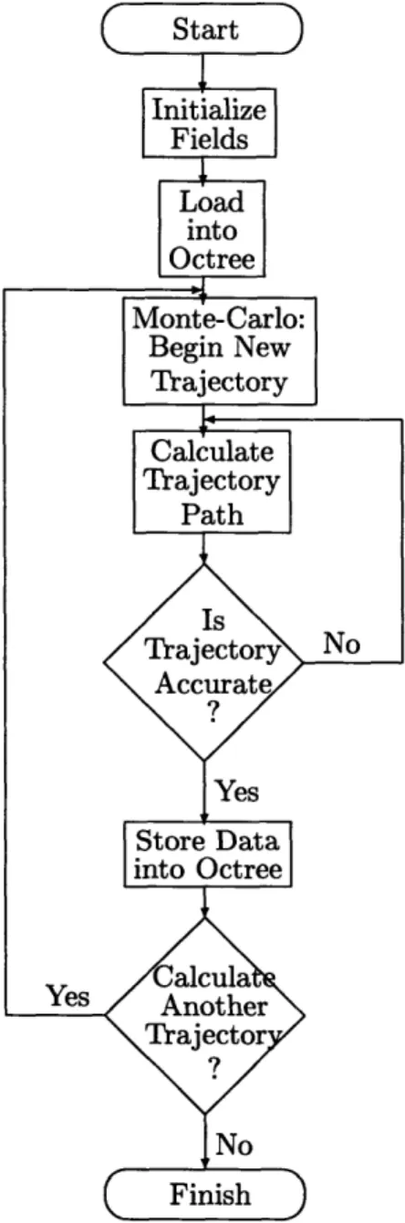
Procedures for calculating current density distributions along a given area of the screen may be condensed onto a simple flow chart Figure 3-1. First, during the initialization stage, electric field values are calculated and loaded into the Octree storage structure. Then, the electron trajectory paths can be calculated, using the electric field values in the Octree lookup table. This simulation process is summarized under the following items:

1. Calculate or load fields of a FED environment 2. Refine fields and store fields into the Octree

3. Use monte carlo to generate an initial electron velocity, under a specific distri-bution

4. Calculate trajectory path through the difference method, using the Octree as a lookup table.

5. Test for trajectory path accuracy, if inaccurate go back to 4. 6. Store trajectory data into Octree

7. Calculate another trajectory path by returning to 3.

Each step performs an important role for determining trajectory paths in a fast and efficient manner.

The first step refers to initializing or scanning in the electric fields. Currently, this is accomplished by analytically determining the field at each desired point within an FED structure. Eventually, this utility will be integrated into MEMCAD, a 3D solid modelling program, which provides a fast and efficient algorithm for calculating fields. MEMCAD will make it easier for the user to define more complex and computationally intensive fields.

Figure 3-1: Virtual-FED Processes: Flow Chart

The ability to quickly incorporate any combination of field values into the system allows for a multitude of different configurations of FED device structures. Thus, the program is versatile enough in nature to embody the fields for any distinctively shaped emitter.

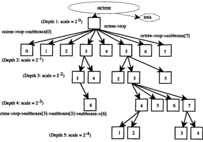
The second item on the list refers to refining and storing the fields into the Octree. This procedure may occur concurrently with the calculation of fields. The Octree is a data-structure, similar to a binary search tree, except it contains eight branches leading from a parent node rather than two branches. And it functions as an efficient table for finding fields, given a position within the environment. In this case, the average computation time for such a search would be O(logg n) as compared to O(n) for the fully degenerate case, where n is the number of nodes within the Octree [13].

Step three begins the trajectory computation stage. After the fields are initialized into the Octree, the monte carlo scheme is used to randomly generate an initial electron velocity vector, under a specified distribution along the emitter tip. Presently, the user may choose to establish a gaussian or uniform distribution for electron inertial vectors normal to the emitter surface at an angle, theta, away from the z-axis.

For the next procedural item, the electron trajectory is calculated through an adaptive difference method, based upon changes in time. That is, the length of the time increment is a function of the refinement for electric fields at a particular position in the FED environment, the velocity of the electron at the previous calculation position, and an initial incremental guess in time. With a determined incremental time, changes in velocity and the next position may be estimated. By default a fourth-order Runge-Kutta method is used, but a linear method may be specified.

The fifth step includes testing for convergence in trajectory path accuracy. Unless the first guess for the incremental time is appropriate, the trajectory path may be inaccurate. For example, if the time increment is too large, the electron may pass through an area of highly varying electric field without being influenced. To correct this, a second trajectory path is calculated with the same input parameters except a finer first guess for incremental time. The two trajectories are then compared, and if the path is found inaccurate to a specified error percentage, a new trajectory path is calculated with an even finer initial guess. Essentially, the Virtual-FED simulation returns back to the previous procedure item, whenever the path is found to be inaccurate.

computed, the Octree functions as a field lookup table; after calculations, the Octree operates as a tabulation, mapping trajectory paths and total electron energies. In the seventh and final item, the decision of calculating a newly specified electron trajectory will return the the procedural stage to the third processing detail: using the Monte-Carlo methods to generate a new initial position and velocity vector.

3.2

Virtual-FED Implementation Details

This section presents an overview of the specific details for implementating the Virtual-FED simulation. The simulation uses several special data constructs and various calcu-lation methods to perform its functions efficiently. The program was implemented under several design considerations. Data structures were devised with both high functionality and performance in mind. The data structure for storing the field values operates as a fast and efficient lookup table. Due to the varying granularity of the fields defined by the FED device settings, the data structures are dynamically allocated when necessary for the efficient usage of memory. Likewise, the data structure for calculating trajectories is also dynamically allocated, so that a desired accuracy of the electron trajectory path may be computed effectively. The following subsections deliver a summary of these special con-structs and some of the simulation methods used. First, a complete description of each special data construct and its function is given. Finally, the implemented computational methods are explored in detail.

3.2.1

Special Constructs

As suggested previously, the simulator defines two major classes of data structures in order to perform rapidly and efficiently. One set of structures, the Octree, is used solely as a table for the storage of field values and trajectory path data. The other data structure, the Trajectory, is used to determine the actual trajectory path of electrons. Special variables have been defined, not very elegantly, in order to keep these two data structures abstracted from one another. For all pratical purposes, these special variables do not effect the program's functionality; however, they do place a few restrictions upon the simulation at its current stage. This is further discussed in the following Section 3.3: Limitations and Restrictions.

Figure 3-2: Top Octree Box

The Octree Data Structure

The Octree data structure stores field values and calculated trajectory path data within the FED device surroundings. The geometry of the environment is assumed to be a cube or rectangular prism. This volume is then mapped into an Octree structure. The entire capacity of the box like structure, may be represented as the top most box in an Octree structure. This top box may be divided into eight equally sized boxes (See figure 3-2). Each of these eight subboxes may further be divided eight times, for a total of 64 boxes defining the FED device.

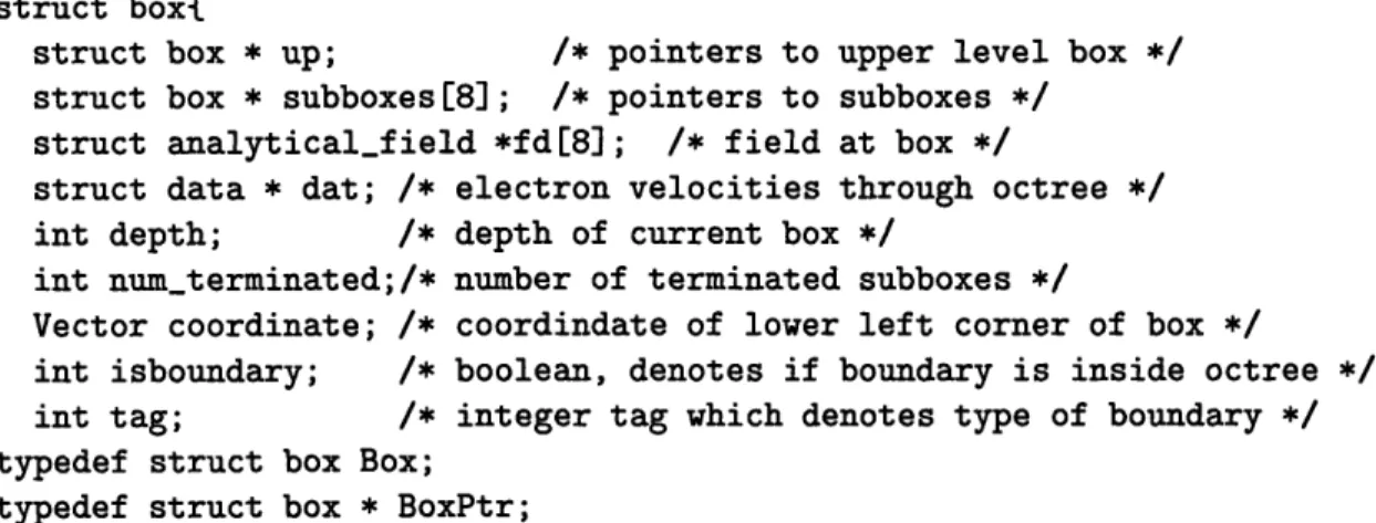
Essentially, the 'Box' element in an Octree is the basic building structure supporting fields and additional data. Other structures are defined inside the Box structure to help organize the data. The C programming language declaration for a Box is shown in Figure 3-3. Also the C declarations for the supporting data structures are listed in Figure 3-4. Below is an inventory of data components for the Box and a description of their functions:

* up - the pointer to the box on the upper level. This field, or component of the Box, in conjunction with the subboxes field define the basis for a double-linked tree structure with eight components, or an Octree.

* subboxes - an array of eight pointers to boxes at a deeper level. A particular subbox is reference in bit-ordered system, where subboxes[xl, x2, x3] is as defined

in Figure 3-2. For example, the subbox positioned at (1, 1, 0) within the top box, can be referenced by subboxes[6].

* fd - an array of eight pointers to the structure that defines an analytical field. Each of these eight fields represent the exact analytical field at one of the eight

struct box{

struct box * up; /* pointers to upper level box */

struct box * subboxes[8]; /* pointers to subboxes */

struct analyticalfield *fd[8]; /* field at box */

struct data * dat; /* electron velocities through octree */ int depth; /* depth of current box */

int num_terminated;/* number of terminated subboxes */

Vector coordinate; /* coordindate of lower left corner of box */

int isboundary; /* boolean, denotes if boundary is inside octree */

int tag; /* integer tag which denotes type of boundary */

typedef struct box Box; typedef struct box * BoxPtr;

Figure 3-3: Box Data Structure

corners of the Box. It is referenced in the same manner as the subboxes.

* dat - pointer to the structure, storing information of the electron trajectory path and total electron energy through the Box.

* depth - the depth of the current box. The depth of the top most box in an Octree is one. This depth increments with each level of subboxes.

* numterminated - the number terminated, or NULL, subboxes from this Box.

* coordinate - the lower left corner position of the Box with respect to the unit-normalized Octree. That is, the top most Box is assumed to have dimensions of unity, and a bottom left hand corner located at the origin.

* isboundary - a boolean that denotes whether a boundary is inside the Box.

* tag - a label, designating a specific type of boundary. The tag may repre-sent a specific surface, such as the emitter or gate surfaces in a FED device environment.

Using boxes as building blocks, Octree is an all inclusive structure, caching fields and trajectory path data. Its primary purpose is to provide an effective field lookup interface to the trajectory calculation functions, mapping positions and scaling the boxes into actual locations within the FED environment. The C programming language declaration for an

struct vector{

double x; /* x component */ double y; /* y component */ double z; /* z component */ typedef struct vector Vector;

struct analyticalfield{

struct vector e; /* Electric field */

struct vector b; /* Magnetic field */

};

typedef struct analyticalfield Afield; struct data{

int num; /* number of electrons passing through box */ double energy; /* total energy of passing electron */

};typedef struct data Data;

typedef struct data Data; typedef struct data * DataPtr;

Figure 3-4: Support Structures for Box

Octree and one supporting data structure is shown in Figure 3-5. The Octree fields are summarized in the following:

* top - the pointer to the top most box. This box has unit dimensions, a Box coordinate of the origin.

* count - total number of boxes in the Octree.

* depth - largest depth in the Octree.

* axis - pointer to the structure with values for mapping positions within the Octree into actual positions.

* isboundary - a boolean that denotes whether a boundary is inside the Octree.

While analyzing a particular FED device, the boxes of an Octree representing areas of highly varying fields may be refined to deeper levels. Whereas, boxes representing less varying fields do not need to be refined. In this manner, the rapidly changing electric fields in the FED device environment are not underepresented, and coarser electric field areas are

struct octree{

struct box *top; /* ptr to top (largest) box */

int count; /* total number of boxes, including all layers */

int depth; /* largest depth */

struct map *axis;/* scale factor for x,y,z axis */

int isboundary; /* boolean, denotes whether boundary is inside octree */

;typedef struct octree Octree;

typedef struct octree

Octree;

typedef struct octree

*

OctreePtr;

struct map{

Vector * scale; /* scale factor for x,y,z axis */

Vector

*

offset; /* lower left hand position */

typedef struct map Map;

typedef struct map * MapPtr;

Figure 3-5: Octree Data-Structures

struct trajelem{

struct trajelem

*

next;

struct trajelem

*

prev;

struct vector pos;

struct vector vel;

double t;

double dt;

/* pointer to next traj.elem */

/* pointer to prev traj.elem */

/* postion vector of particle */

/* velocity vector of particle */

/*

total time elapsed */

/* increment in time */

typedef struct traj;elem Listelem;

typedef struct trajelem

ListelemPtr;

typedef struct trajelem

*

List;

typedef struct traj-elem * List;

struct trajectory{

int num;

struct trajelem

*

front;

struct traj-elem

*

rear;

struct trajelem

arry;

/* total number of trajelem's */

/* pointer to first elem of list*/

/* pointer to last elem of list*/

/* arry of trajectory elements */

};typedef struct trajectory Trajectory;

typedef struct trajectory Trajectory;

typedef struct trajectory * TrajectoryPtr;

Figure 3-7: Trajectory Data-Structures

not needlessly over-represented, such that the octree provides a fast and efficient lookup table for fields. (For example, see Figure 3-6)

Trajectory Data-Structures

The second main data structure, or the Trajectory structure, calculates trajectory paths using field values stored within the Octree. The basic building block for the Trajectory is a traj elem, or Listelem. It operates as a double-linked list of Listelems, basically functioning as a queue. The C programming language declaration for a Trajectory and its supporting structure is shown in Figure 3-7. Below is a list of data components of the Listelem and a brief description of functionality. A simple conceptual diagram is given in Figure 3-8.

* next and prev - pointers to other Listelems. These fields are used to form a double-linked list of Listelems, creating a queue.

TrajectoryPtr

num front rear a-ry

front trajectory j1

(total

time=O)

Figure 3-8: Diagram of Trajectory Structure

* pos - electron vector position with respect to the origin inside the FED envi-ronment.

* vel - electron vector velocity at given instance of time.

* t - total time elapsed, upon entering the current vector position.

* dt - increment in time, used to calculate the next trajectory item. Hence the total time for the next trajectory element, is t + dt.

3.2.2

Octree Field Estimation

For reasons of precision, the fields stored inside an Octree box must be representative of the field for the entire box. The Box structure within an Octree contains field values for each of its eight verticies. When field lookup is specified for a point within the volume of the box, a three-dimensional, linear interpolation of the fields is returned.

3.2.3

Trajectory Convergence Implementation

The first calculation of the trajectory path may be inaccurate, unless the original initial guess in incremental time is appropriate. In order to test for accuracy, a second trajectory path is calculated with the same input parameters with the exception of a finer initial guess for incremental time. The two trajectories are then compared by sampling both trajectories at the same instances in time, and identifying the maximum length of vector difference between two positional points. This maximum length represents the largest interval of error between the two trajectories. This is given by Equation 3.1. Next, the maximum length is normalized against the dimensions of the FED structure in order to ensure that all three axes have equal weight, and weighed with the maximum allowable percentage of

Y

Figure 3-9: Semi-Circular Cone Emitter

error specified by the user.

3

S=

max{Ia-bnI}

=

max{I

I}

(3.1)

where n represent the sample number.

3.2.4

Monte Carlo Implentation

The Monte-Carlo method is used to initialize the velocity and position vectors for an elec-tron trajectory, and it generates either a uniform or normal gaussian distribution of initial velocity at emitter tip surface. The initial position for the electron trajectory is located within an angle, 0, away from the z-axis, along the surface of the emitter. The original electron velocity vector is normal to the suface of the initial position (See figure 3-9). For the purposes of this work, the distribution in € was assumed to be uniform around the emitter. The implementation of the monte-carlo methodology for a uniform distribution is a trivial matter. However, for a gaussian distribution, it is more complicated. The normal gaussian probability density function defined by:

fo(0)

2a2

used to determine whether to make a trajectory call at a particular (randomly generated)

8 [14]. Bayes's theorem states: given a known gaussian probability density function for 0

and fo(0), then the probability of event A (in this case, the event that the trajectory with an initial velocity vector directed

0

0 took on the value 0 is:

Pr(AjO = 0) = fo(01A)Pr(A) (3.3)

fo(0)

3.3

Limitations and Requirements

With infinite memory, there are no limitations on the number of Trajectory structures or Octree boxes that may be generated. However, the simulations are restricted based upon computer memory limitations. In particular, boxes within the Octree data structure, require much memory in order to map the FED environment. This is true, even with the feature of selective refining inside the Octree. In fact, one Box structure claims 504 bytes of memory, and for any simulation result described in Chapter 4, 86,665 Octree boxes are necessary in order to accurately map the FED device surroundings. Thus, over 43.6 MBytes are necessary to map the Octree structure alone for those graphs.

As discussed earlier, special variables have been defined to keep these the Octree and Trajectory data structures abstracted from one another. The restrictions to the program is that fields cannot be recalculated anaytically, while using the same Octree as a lookup table. Also at any one period in time, only one Octree structure may be in existence. It may pose a problem when FEAs are to be implemented, since more than one Octree structure may need to be referenced at any one time. Nonetheless, the current implementation can be easily altered if necessary.

3.4

Virtual-FED Usage

The simulation code is intended to serve as a library in the C programming language for calculating various FED charateristics, such as the spot size of on the screen. Most of the procedures for calculating uniform and gaussian distributions are written. See the Appendicies for the Virtual-FED program and documentation. The user needs only to follow a simple procedure, common to many programs:

1. Initialize variables - device geometry values, fields, and Octree refinement. 2. Perform desired calculations

3. Output results 4. Free variables

Parameter Initialization

Before any trajectory calculations can be made, the user must initialize several data struc-tures and other variable parameters. The data strucstruc-tures for these parameters are listed in Figure 3-10. These structures are described briefly below:

* Fields - field structure which has two components. One which contains an analytical field expression, or the field value itself. The other is a pointer to the Octree. The data structure of the analytical field was given in Figure 3-4.

* Initiale - the initial electron data structure, contains information such as the electron charge, mass, initial position before trajectory calculation, and initial velocity before trajectory calculation.

* Bounds - the boundaries for simulated volume are stored here.

In addition, the user must refine areas of interest in the FED device. There are a number of functions, defined in the Virtual-FED utility, which specializes in refining the octree. These function prototypes are listed below as well as in 'Appendix C: octree.m.'

* refine - given a depth, or number of levels to refine, this function refines the entire FED device volume to the number specified by depth.

* refine2perc - refines the entire FED device volume to the level of boxes, having a common parent box, with a specified percentage of variation between their fields. Note, that this function may overlook highly varying field points or singularities in the volume.

* refine2point - given a depth, this function refines to a specified position in the volume.

struct field_struct{ struct analytical_field af; /* analytical fields

*/ struct octree * oct; /* fields stored on an octree */ }; typedef

struct fieldstruct Fields;

struct initiale{

double q;

double m;

struct vector pos;

struct vector vel;

}; typedef struct struct bounds{ double xmax; double xmin; double ymax; double ymin; double zmax; double zmin; typedef struct

/* charge of particle

*/

/* mass of particle */

/* intial postion vector of particle */

/* intial velocity vector of particle */

initiale Initiale;

value

value

value

value

value

value

bounds Bounds;

Figure 3-10: Virtual-FED: Structures User Must Initialize

* refine2pointperc - given a percentage for the variation of field values, this function refines the Octree at a specified position to a level where neighboring subboxes fall within the percentage of field variation.

* refinebds - refines the boundaries of a box at specified incremental values.

* refinetopbds - refines uniformly at the top of the Octree, where the phosphor screen is located.

* refinesemi - refines a semi-circle above the x-y plane. This semi-circle is centered about the origin.

Perform Calculations

There are a few higher-order functions which specialize in generating electron trajectories. Their prototypes are listed 'Appendix A: trajectory.h.' A brief description of each are given in bullet form below:

* transit - calculates a single electron trajectory.

* uniform_dist - calculates trajectories with a uniform distribution of initial velocities; the uniform distribution is defined with respect to the range of 8.

* gaussiandist - calculates trajectories with gaussian distribution of initial velocities.

Output Results

There are two functions which print out the results, which are stored in the Octree structure. These functions are listed in 'Appendix C: octree.h.' and also described below:

* printboxdata - print the data from each and every Octree box.

* print_topdat2file - print data from the screen into a file.

Freeing Variables

After trajectories have been calculated and the results written to file, it is necessary to free certain variables. In particular, the Octree and the Trajectory data structures need to be freed. The following two procedures will free the Octree and the Trajectory structures respectively.

* destroy_octree - destroys the Octree data structure.

* destroytrajectory - destroys the Trajectory data structure.

Sample FED Trajectory Program

Figure 3-11 represents a Virtual-FED sample program, which is used to calculate the results for uniform distibution functions, described in the next chapter. For the user, the most tedious procedure can be initializing the input values into the program. In this case, an inputfile could be helpful.

/* Virtual-FED Sample Program

*/

#include "trajectory.m"

void main()

TrajectoryPtr t; /* trajectory pointer */

Initiale ch; /* initial electron information */

Bounds bd; /* boundary information */

Fields f; /* fields structure */

Afield af; /* analytical field structure ,/

double maxerror; /* maximum allowable error between two trajectories */ double energy; /* magnitude of inital trajectory energy */

int num_traj; /* the desired number of trajectory calls */

char s[50]; /* filename, cannot be more than 49 characters long */ /* scan in values for:

V_a = anode voltage (in volts) V_g = gate voltage (in volts)

energy = initial electron energy (eV) numtraj = number of desired trajectores

s = string, or filename to write data into

scanf("%lf %lf %lf %d %7s", &VA, &VG, &energy, &num_traj, s); the init-all fuction will prompt the user for various parameters

such as the electron information, the boundaries of the environment initial fields, maximum allowable error between similar trajectory paths, a refinement levels within the Octree are also prompted as

a user inDut.

initall(&t, &ch, &bd, &f, &af, &maxerror);

this fuction writes into the octree and calculates a uniform distribution of initial velocities normal to the surface of the emitter, with the characteristics of previously discussed variables, within the range of 0.0 < theta < 2.0

uniformdist(ch, f, bd, maxerror, energy, numtraj, 2.0);

/* prints only data from the top of the screen to a datafile */

printtopdata2file(oct->top, oct, bd, s); destroyoctree(oct); /* free memory */