HAL Id: inserm-00663764
https://www.hal.inserm.fr/inserm-00663764
Submitted on 27 Jan 2012
HAL is a multi-disciplinary open access
archive for the deposit and dissemination of
sci-entific research documents, whether they are
pub-lished or not. The documents may come from
teaching and research institutions in France or
abroad, or from public or private research centers.
L’archive ouverte pluridisciplinaire HAL, est
destinée au dépôt et à la diffusion de documents
scientifiques de niveau recherche, publiés ou non,
émanant des établissements d’enseignement et de
recherche français ou étrangers, des laboratoires
publics ou privés.
To cite this version:
Sigrid Rouam, Thierry Moreau, Philippe Broët. Identifying common prognostic factors in genomic
cancer studies: a novel index for censored outcomes.. BMC Bioinformatics, BioMed Central, 2010, 11
(1), pp.150. �10.1186/1471-2105-11-150�. �inserm-00663764�
© 2010 Rouam et al; licensee BioMed Central Ltd. This is an Open Access article distributed under the terms of the Creative Commons Attribution License (http://creativecommons.org/licenses/by/2.0), which permits unrestricted use, distribution, and reproduction in any medium, provided the original work is properly cited.
Identifying common prognostic factors in genomic
cancer studies: A novel index for censored
outcomes
Sigrid Rouam*
1,2, Thierry Moreau
3and Philippe Broët
1,2Abstract
Background: With the growing number of public repositories for high-throughput genomic data, it is of great interest to combine the results produced by independent research groups. Such a combination allows the identification of common genomic factors across multiple cancer types and provides new insights into the disease process. In the framework of the proportional hazards model, classical procedures, which consist of ranking genes according to the estimated hazard ratio or the p-value obtained from a test statistic of no association between survival and gene expression level, are not suitable for gene selection across multiple genomic datasets with different sample sizes. We propose a novel index for identifying genes with a common effect across heterogeneous genomic studies designed to remain stable whatever the sample size and which has a straightforward interpretation in terms of the percentage of separability between patients according to their survival times and gene expression measurements.
Results: The simulations results show that the proposed index is not substantially affected by the sample size of the study and the censoring. They also show that its separability performance is higher than indices of predictive accuracy relying on the likelihood function. A simulated example illustrates the good operating characteristics of our index. In addition, we demonstrate that it is linked to the score statistic and possesses a biologically relevant interpretation. The practical use of the index is illustrated for identifying genes with common effects across eight independent genomic cancer studies of different sample sizes. The meta-selection allows the identification of four genes (ESPL1, KIF4A, HJURP, LRIG1) that are biologically relevant to the carcinogenesis process and have a prognostic impact on survival outcome across various solid tumors.
Conclusion: The proposed index is a promising tool for identifying factors having a prognostic impact across a collection of heterogeneous genomic datasets of various sizes.
Background
In clinical cancer research, recent advances in genome-wide technologies have enabled researchers to identify large-scale genomic changes having a potential prognostic impact on time-to-event outcomes. The growing number of public repositories for high-throughput genomic data facilitates the retrieval and combination of various datasets produced by independent research groups (for a few: GEO [1], Oncomine [2], ArrayExpress [3]). These databases poten-tially represent valuable resources for identifying genomic factors that have a common prognostic impact on clinical
outcomes (e.g. time to local or distant recurrence) across multiple cancer types. However, the joint analysis of these heterogeneous datasets is difficult due to the fact that they are usually of varying sample size, investigate different sur-vival outcomes or are related to different tumors entities. In this context, defining a procedure for identifying common genomic risk factors across multiple heterogeneous datasets is a promising but very challenging task. In recent years, several authors [4-7] have proposed meta-profiling methods for class comparison, designed to identify common tran-scriptional features of the tumoral process (normal versus tumor state).
In the framework of the widely used Cox model [8] for analyzing possibly censored time-to-event or survival data, * Correspondence: sigrid.rouam@inserm.fr
1 Computational and Mathematical Biology, Genome Institute of Singapore, Singapore 138672, Singapore
gene expression datasets can be defined. Basically, each gene expression measurement is included in a simple Cox model, giving rise to an estimation of the corresponding hazard ratio and to a statistic for testing the null hypothesis of no association between survival outcome and gene expression changes. Simple procedures, frequently used in practice, consist of ranking the genes in each dataset from the highest (or lowest) value to the lowest (or highest) value according to either the estimated hazard ratio or quantities derived from the test statistic (e.g. p-value), and finally to select those that appear at the intersection of the lists using a defined thresholding procedure [9]. However, these approaches suffer serious drawbacks that are mostly related to the chosen selection criteria. Choosing the estimated haz-ard ratio clearly ignores the variability of the data, while the choice of quantities derived from test statistics leads to emphasize large datasets, since it is well known that every test statistic increases with the sample size.
In meta-selection of heterogeneous genomic datasets, tak-ing into account both the magnitude of the prognostic impact of factors and the variability of the data without being highly dependent on the sample size is likely to be more biologically relevant. Addressing this issue led us to propose a novel index designed for genomic survival analy-sis that provides information about the capability of a genomic factor to separate patients according to their time-to-event outcome. Our work shares conceptual links with the framework of predictive ability measures that aim to determine which covariates have the greatest explanatory interest. For censored data, two main frameworks have been proposed for quantifying the predictive ability of a variable to separate patients: (i) concordance, which quanti-fies the degree of agreement among the ranking of observed failure times according to the explained variables and is used to assess the discriminatory performance of a model [10,11]; (ii) proportion of explained variation, which quan-tifies the relative gain in prediction ability between a cova-riate-based model and a null model (without explained variables) by analogy with the well-known linear model. In this latter case, two approaches have been considered. The first one focuses on comparing empirical survival functions with and without covariates [12-15]. The second one con-siders statistical quantities which are directly or indirectly related to the likelihood function [16-19]. In this paper, we propose a novel index that is linked to the approach dis-cussed above. It is related to the score statistic and well-suited for meta-selection of genomic datasets. Our index is interpreted as the ability of a gene to separate patients observed to experience the event of interest from those who do not experience the event among the risk set at every observed failure time. As shown in this study, increasing values of the index correspond to a higher effect due to the gene variable. In contrast to a test statistic, our index is not
well-suited for meta-selection from datasets with various sample sizes.
We report and discuss the statistical properties of the index obtained from simulation experiments, and compare it to Allison's index [16] and its modified version [18], Nagelkerke [17] and Xu and O'Quigley's [19] indices. In addition, the properties of these indices are illustrated on a fictitious example, where data are simulated so as to mimic a real study combining datasets of different sample sizes. We then illustrate the capability of the index for combining the results of eight cancer studies of different sample sizes and with different outcomes.
Results
Statistical properties of the proposed index and comparison with classical indices
Simulation Scheme
A simulation study was performed to evaluate the behavior of the proposed index, denoted and compare it to Alli-son's index [16], a modified version of AlliAlli-son's index [18], Nagelkerke [17] and Xu and O'Quigley's [19] indices
denoted and respectively (see the
Methods Section for the description of the five indices) under proportional and non-proportional hazards regression models, using different values of the regression parameter, different covariate distributions and different sample sizes. Scenarios with various independent censoring distributions were also considered.
The simulation protocol was as follows. For each subject i, i = 1,傼, n, we considered one covariate Z with either a discrete (Bernoulli V(0.5)) or a continuous (uniform [0, ]) distribution. These two distributions of Z were standardized to have the same variance. Survival times T were generated with the survival function S(t; z) = exp(-teβZ) (proportional hazards model) or S(t; z) = (1 + t · eβZ)-1 (proportional odds model). For these two survival distribu-tions, the hazard ratios were HR = eβ for the proportional hazard model and HR = [1 + (eβ - 1)S
0(t)]-1 for the propor-tional odds model, S0(t) refering to the baseline survivor function. In our simulation scheme, eβ was set to 1 (null effect), to small values; 1.25, 1.5, 1.75, medium values; 2, 3, and high values; 4, 5. The sample sizes n of the data were taken equal to 50, 100, 500 and 1, 000.
The censoring mechanism was assumed to be indepen-dent from T given Z and the distribution of the censoring variable Ci, i = 1,傼, n was either uniform Ci ~ {0, r} or exponential Ci~ {γ }. The calculation of the parameters r and γ as functions of the expected overall percentage of censoring pc is described in Additional file 1. The
percent-D0∗ ρ ρN2, k2,RN2 ρXOQ2 U ( )3 U E
ulations for for four different sample sizes and two dif-ferent covariate distributions, considering a Cox proportional hazards model. As seen from Additional file 2, when β = 0, i.e. in the absence of covariates, our index approaches 0 for n = 50 to 1, 000; the separability is close to 0. The index increases towards 1 with |β|, the separability increases with the effect of the covariate. When β≠ 0, the value of for the different sample sizes is fairly stable, in particular for moderate or high effects (eβ ≥ 1.5). The mean values of our index for n = 50 to 500 are close to the mean values obtained for n = 1, 000 which is assumed to approach its asymptotic limit. The standard errors of (indicated in brackets in Additional file 2) are small even when censored, and, as expected, decrease when n increases. Our index is slightly sensitive to the censoring rate, especially for high values of hazard ratio. Similar com-ments can be made when dealing with an exponential cen-soring mechanism (results not shown).
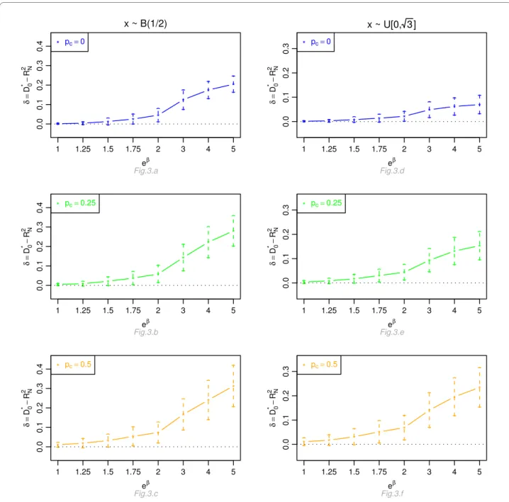
Figures 1, 2, 3 and 4 display, for a Cox model, the
differ-ences δ between the mean of and the mean of
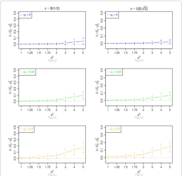
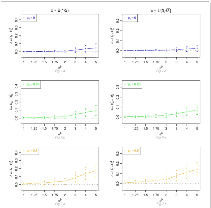
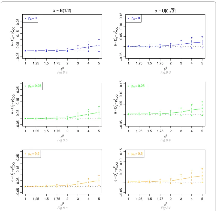
and respectively, for n = 100, for dif-ferent percentage of censoring pc, different covariate distri-butions and with a uniform censoring mechanism. The means of the differences δ are always positive. They are close to zero for small hazard ratios and increase with higher hazard ratios. The differences between and increase with the percentage of censoring, which is not sur-prising since the Nagelkerke's index is known to be sensi-tive to censoring [15]. The two indices and have a similar behavior relatively to . This is expected since O'Quigley et al [18] propose to use as a simple working approximation of their index. The same results are obtained for n = 50, 500 and 1, 000 and for an exponential censoring mechanism (results not shown). For eβ ≥ 2, the 95% confi-dence interval for the differences of the three graphs does not comprise 0, thus in each case the difference δ is signifi-cant. The table in Additional file 3 and Figures 5, 6, 7 and 8 display the results of the simulations under a proportional odds model. The mean values of the different indices are lower than in the case of a proportional hazards model. All indices are more sensitive to censoring. Our index shows higher mean values than the other indices, especially in case of a Bernoulli distribution.
practical interest of our index when combining the information contained in two studies with different sample sizes. The method used to generate the two datasets was inspired by Bair and Tibshirani [20] but modified in order to resemble the structure of real genomic data. The two datasets mimicked the analysis of the prognosis impact of transcriptional changes for a set of 1, 000 genes. The two datasets were of unequal size and composed of n = 150 and 50 individuals, respectively. To each individual i, i = 1,傼, n; n = 150 or 50, we associated a survival time Ti, a censoring time Ci and vector of 1,000 quantitative values Zi = { ; g = 1,傼, 1, 000} (e.g. expression measurement).
To perform a fair evaluation of our index, we simulated survival data with either an exponential distribution given by S(t) = exp(-teξ) (proportional hazard model) or a log-logistic survival distribution given by S(t) = (1 + t · eξ)-1 (non-proportional hazard model). For individuals i such as 1 ≤ i ≤ n/2 (n = 150 or 50), the parameter ξ was equal to 0. For individuals i such as n/2 + 1 ≤ i ≤ n (n = 150 or 50), eξ was equal to 3 and 5. We defined individuals i = 1 to n/2 as belonging to the group of patients with low risk of occur-rence of the event of interest and individuals from i = n/2 + 1 to n to the group with high risk of occurrence of the event. For each dataset, censoring times Ci (i = 1,傼, n; n = 150 or 50) were considered independent from survival times and with a uniform distribution on {0, r}, r chosen in order to have an expected percentage of censoring of 30%.
The observed time to follow-up (i = 1,傼, n; n = 150 or 50) was equal to the minimum between the two previ-ously defined times Ti and Ci.
For the two datasets, for each individual i, 1,000 gene expression values (i = 1,傼, n; n = 150 or 50; g = 1,傼, 1, 000) were generated, according to the simulation scheme shown on the figure in Additional file 4. Gene expression values from g = 1 to 50 for individuals i = 1 to n/2 (n = 150 or 50) followed a log-normal distribution Log- (μ = 4, σ
= 1.5) with and
. For the rest of the individuals (i = n/2 + 1,傼, n; n = 150 or 50), gene expression values fol-lowed a distribution Log- (0, 1.5). Gene expression val-ues from g = 51 to 100 for individuals i = 1 to n/2 (n = 150 or 50) followed a log-normal distribution with parameters μ = 3 and σ = 1.5 Log- (3, 1.5). For the rest of the individ-uals (i = n/2 + 1,傼, n; n = 150 or 50), gene expression val-ues followed a distribution Log- (0, 1.5). For gene D∗0 D0∗ D0∗ D0∗ ρ ρN2, k2,RN2 ρXOQ2 D0∗ RN2 ρk2 ρ XOQ 2 D0∗ ρk2 D0 Zi( )g Ti∗ Xi( )g N E X( )=eμ+0 5.σ2 V X( )=e2μ σ+ 2(eσ2 −1) N N N
expression values from g = 100 to 150 and for 40% individ-uals randomly selected among the n (n = 150 or 50), the (i 8 N, g = 100,傼, 150) followed a log-normal distri-bution Log- (1, 1.5), whereas for the remaining individu-als, they followed a log-normal distribution Log- (0, 1.5). For gene expression values from g = 151 to 250 and
for 50% individuals randomly selected among the n, the (i 8 N; g = 151,傼, 250) followed a log-normal distri-bution Log- (0.5, 1.5), whereas for the remaining indi-viduals, they followed a log-normal distribution Log- (0, 1.5). For gene expression values from g = 251 to 350 and for 70% individuals randomly selected among the n, the Xi( )g N N Xi( )g N N Figure 1 Graphic of the differences δ between the mean values of and the mean values of as a function of the hazard ratio, for a Cox proportional hazards model. Mean of as a function of the relative risk eβ, for different percentages of censoring p
c, for a covariate
with Bernoulli V(1/2) or uniform [0, ] distribution, n = 100 and a uniform censoring mechanism.
* * * * * * * * 0.0 0.1 0.2 0.3 0.4 0.5 x ~ B(1/2) eβ δ= D0 * −ρ N 2 Fig.1.a 1 1.25 1.5 1.75 2 3 4 5 * pc= 0 * * * * * * * * 0.0 0.1 0.2 0.3 0.4 0.5 eβ δ= D0 * −ρ N 2 Fig.1.b 1 1.25 1.5 1.75 2 3 4 5 * pc= 0.25 * * * * * * * * 0.0 0.1 0.2 0.3 0.4 0.5 eβ δ= D0 * −ρ N 2 Fig.1.c 1 1.25 1.5 1.75 2 3 4 5 * pc= 0.5 * * * * * * * * 0.0 0.1 0.2 0.3 0.4 x ~ U[0, 3] eβ δ= D0 *−ρ N 2 Fig.1.d 1 1.25 1.5 1.75 2 3 4 5 * pc= 0 * * * * * * * * 0.0 0.1 0.2 0.3 0.4 eβ δ= D0 *−ρ N 2 Fig.1.e 1 1.25 1.5 1.75 2 3 4 5 * pc= 0.25 * * * * * * * * 0.0 0.1 0.2 0.3 0.4 eβ δ= D0 *−ρ N 2 Fig.1.f 1 1.25 1.5 1.75 2 3 4 5 * pc= 0.5 D0∗ ρN2 D∗0− ρN2 U ( )3
(i 8 N; g = 251,傼, 350) followed a log-normal distri-bution Log- (0.1, 1.5), whereas for the remaining indi-viduals, they followed a log-normal distribution Log- (0, 1.5). Finally, for gene expression values from g = 351 to 1,
000, the (i = 1,傼, n; g = 351,傼, 1, 000) followed a log-normal distribution Log- (0, 1.5) for all individuals.
As genes involved in the same or related pathway are likely to be coexpressed, we introduced correlations between genes. To evaluate the behavior of our index in the context of dependent data, we generated datasets with so-called "clumpy" dependence (gene measurements are Xi( )g
N
N
Xi( )g
N
Figure 2 Graphic of the differences δ between the mean values of and the mean values of as a function of the hazard ratio, for a Cox proportional hazards model. Mean of as a function of the relative risk eβ, for different percentages of censoring p
c, for a covariate
with Bernoulli V(1/2) or uniform [0, ] distribution, n = 100 and a uniform censoring mechanism.
* * * * * * * * −0.05 0.05 0.15 0.25 eβ δ= D0 * −ρ k 2 Fig.2.a 1 1.25 1.5 1.75 2 3 4 5 * * * * * * * * −0.05 0.05 0.15 0.25 eβ δ= D0 * −ρ k 2 Fig.2.b 1 1.25 1.5 1.75 2 3 4 5 * pc= 0.25 * * * * * * * * −0.05 0.05 0.15 0.25 eβ δ= D0 * −ρ k 2 Fig.2.c 1 1.25 1.5 1.75 2 3 4 5 * pc= 0.5 * * * * * * * * −0.05 0.05 0.10 eβ δ= D0 *−ρ k 2 Fig.2.d 1 1.25 1.5 1.75 2 3 4 5 * * * * * * * * −0.05 0.05 0.10 0.15 eβ δ= D0 *−ρ k 2 Fig.2.e 1 1.25 1.5 1.75 2 3 4 5 * pc= 0.25 * * * * * * * * −0.05 0.05 0.10 0.15 eβ δ= D0 *−ρ k 2 Fig.2.f 1 1.25 1.5 1.75 2 3 4 5 * pc= 0.5 D0∗ ρk2 D0∗ − ρk2 U ( )3
dependent in small groups, but each group is independent from the others). We applied the following protocol [21,22]. For each group of ten genes indexed by l, l = 1,傼, 100, a random vector A = ail, i = 1,傼, n, was generated from a standard log-normal distribution Log- (0, 1). The data
matrix Z was then built so that
with ρ equal to 0.25, 0.5 or 0.75. Finally and in order to show the behavior of our index in situations close to real genomic data analysis, we standardized the dataset using classical quantile normaliza-tion [23].
In this simulation scheme, the first hundred genes were differentially expressed between the low and high risk N
Zilg Ail Xil
g
( )= ρ ⋅ + − ⋅ρ ( )
1
Figure 3 Graphic of the differences δ between the mean values of and the mean values of as a function of the hazard ratio, for a Cox proportional hazards model. Mean of as a function of the relative risk eβ, for different percentages of censoring p
c, for a covariate
with Bernoulli V(1/2) or uniform [0, ] distribution, n = 100 and a uniform censoring mechanism.
* * * * * * * * 0.0 0.1 0.2 0.3 0.4 x ~ B(1/2) eβ δ= D0 * − RN 2 Fig.3.a 1 1.25 1.5 1.75 2 3 4 5 * pc= 0 * * * * * * * * 0.0 0.1 0.2 0.3 0.4 eβ δ= D0 * − RN 2 Fig.3.b 1 1.25 1.5 1.75 2 3 4 5 * pc= 0.25 * * * * * * * * 0.0 0.1 0.2 0.3 0.4 eβ δ= D0 * − RN 2 Fig.3.c 1 1.25 1.5 1.75 2 3 4 5 * pc= 0.5 * * * * * * * * 0.0 0.1 0.2 0.3 x ~ U[0, 3] eβ δ= D0 *− RN 2 Fig.3.d 1 1.25 1.5 1.75 2 3 4 5 * pc= 0 * * * * * * * * 0.0 0.1 0.2 0.3 eβ δ= D0 *− RN 2 Fig.3.e 1 1.25 1.5 1.75 2 3 4 5 * pc= 0.25 * * * * * * * * 0.0 0.1 0.2 0.3 eβ δ= D0 *− RN 2 Fig.3.f 1 1.25 1.5 1.75 2 3 4 5 * pc= 0.5 D0∗ RN2 D0∗ − RN2 U ( )3
group of patients. The other 250 genes were not linked to the low and high risk status, but were distributed differen-tially according to a binary factor (with various means) unlinked to the low/high risk status. The remaining genes were not linked to the low and high risk status.
For a given threshold, we calculated the number of genes common to the two simulated datasets with the five indices,
for the different survival distributions, the different hazards ratio values and the different correlations between genes. We estimated the true positive fraction (TPF, number of true positives found divided by the number of truly prog-nostic genes) and the true negative fraction (TNF, number of true negatives divided by the number of truly non-prog-nostic genes) obtained with the five indices, D0∗, Figure 4 Graphic of the differences δ between the mean values of and the mean values of as a function of the hazard ratio, for a Cox proportional hazards model. Mean of as a function of the relative risk eβ, for different percentages of censoring p
c, for a
cova-riate with Bernoulli V(1/2) or uniform [0, ] distribution, n = 100 and a uniform censoring mechanism.
* * * * * * * * −0.05 0.05 0.15 0.25 eβ δ= D0 * −ρ XOQ 2 Fig.4.a 1 1.25 1.5 1.75 2 3 4 5 * * * * * * * * −0.05 0.05 0.15 0.25 eβ δ= D0 * −ρ XOQ 2 Fig.4.b 1 1.25 1.5 1.75 2 3 4 5 * pc= 0.25 * * * * * * * * −0.05 0.05 0.15 0.25 eβ δ= D0 * −ρ XOQ 2 Fig.4.c 1 1.25 1.5 1.75 2 3 4 5 * pc= 0.5 * * * * * * * * −0.05 0.05 0.10 eβ δ= D0 * −ρ XOQ 2 Fig.4.d 1 1.25 1.5 1.75 2 3 4 5 * * * * * * * * −0.05 0.05 0.10 0.15 eβ δ= D0 * −ρ XOQ 2 Fig.4.e 1 1.25 1.5 1.75 2 3 4 5 * pc= 0.25 * * * * * * * * −0.05 0.05 0.10 0.15 eβ δ= D0 * −ρ XOQ 2 Fig.4.f 1 1.25 1.5 1.75 2 3 4 5 * pc= 0.5 D0∗ ρXOQ2 D0∗ − ρXOQ2 U ( )3
and as a function of the threshold target value. These criteria were estimated by the mean over one hundred iterations of: (i) the proportion of correct selection (i.e. when the selected genes g belonged to {0,傼, 100}) among the modified genes; (ii) the proportion of correct 'non-selection' (i.e. when the selected genes g belonged to
{101,傼, 1, 000}) among the non-modified genes, respec-tively.
Considering this procedure, the most successful criterion was the one that achieve the best operating characteristics. Simulation Results
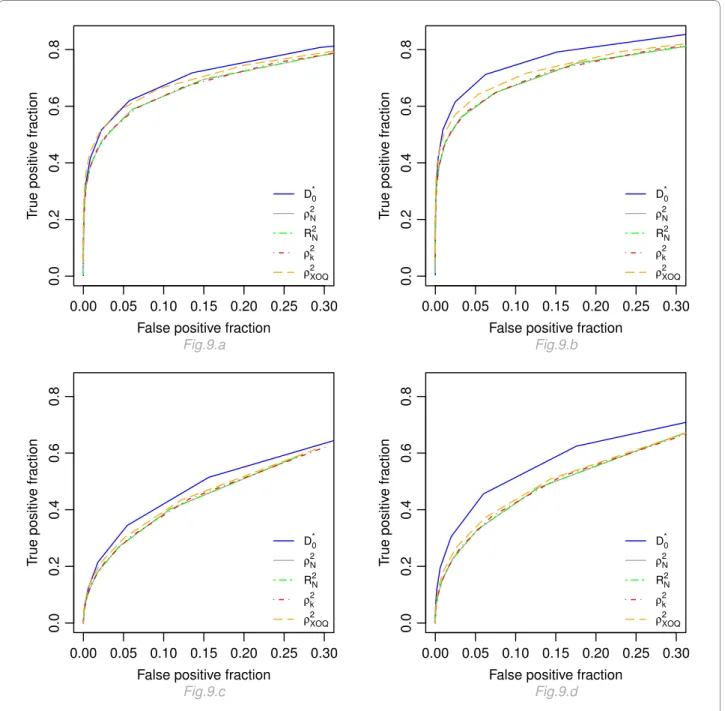
Figure 9 displays the true positive fraction versus the false negative fraction (number of false positives found divided by the number of truly non-prognostic genes) for four con-ρ con-ρN2, k2,RN2 ρXOQ2
Figure 5 Graphic of the differences δ between the mean values of and the mean values of as a function of the odds ratio, for a proportional odds model. Mean of as a function of the odds ratio eβ, for different percentages of censoring p
c, for a covariate with
Ber-noulli V(1/2) or uniform [0, ] distribution, n = 100 and a uniform censoring mechanism.
* * * * * * * * 0.0 0.1 0.2 0.3 0.4 0.5 x ~ B(1/2) eβ δ= D0 * −ρ N 2 Fig.5.a 1 1.25 1.5 1.75 2 3 4 5 * pc= 0 * * * * * * * * 0.0 0.1 0.2 0.3 0.4 0.5 eβ δ= D0 * −ρ N 2 Fig.5.b 1 1.25 1.5 1.75 2 3 4 5 * pc= 0.25 * * * * * * * * 0.0 0.1 0.2 0.3 0.4 0.5 eβ δ= D0 * −ρ N 2 Fig.5.c 1 1.25 1.5 1.75 2 3 4 5 * pc= 0.5 * * * * * * * * 0.0 0.1 0.2 0.3 0.4 x ~ U[0, 3] eβ δ= D0 *−ρ N 2 Fig.5.d 1 1.25 1.5 1.75 2 3 4 5 * pc= 0 * * * * * * * * 0.0 0.1 0.2 0.3 0.4 eβ δ= D0 *−ρ N 2 Fig.5.e 1 1.25 1.5 1.75 2 3 4 5 * pc= 0.25 * * * * * * * * 0.0 0.1 0.2 0.3 0.4 eβ δ= D0 *−ρ N 2 Fig.5.f 1 1.25 1.5 1.75 2 3 4 5 * pc= 0.5 D0∗ ρN2 D0∗ − ρN2 U ( )3
figurations: ρ = 0.5, eξ = 3 and 5 and for a proportional and non-proportional model. For the five indices, higher operat-ing characteristics are obtained under a proportional haz-ards model (Figure 9.a and 9.b) as compared to a proportional odds model (Fig 9.c and 9.d). Moreover, for a given distribution and a given threshold, our index gives the best results with higher true positive and true negative frac-tions. Results for the four other indices are very close to
each other. Results with other levels of correlation (ρ = 0.25 and 0.75) are very close to those obtained with ρ = 0.5 (curves not shown here).
Application of the index on real data
Datasets
In this section, we exemplify the use of the proposed index by identifying transcriptomic prognostic factors common to Figure 6 Graphic of the differences δ between the mean values of and the mean values of as a function of the odds ratio, for a proportional odds model. Mean of as a function of the odds ratio eβ, for different percentages of censoring p
c, for a covariate with
Ber-noulli V(1/2) or uniform [0, ] distribution, n = 100 and a uniform censoring mechanism.
* * * * * * * * −0.05 0.05 0.15 0.25 eβ δ= D0 * −ρ k 2 Fig.6.a 1 1.25 1.5 1.75 2 3 4 5 * * * * * * * * −0.05 0.05 0.15 0.25 eβ δ= D0 * −ρ k 2 Fig.6.b 1 1.25 1.5 1.75 2 3 4 5 * pc= 0.25 * * * * * * * * −0.05 0.05 0.15 0.25 eβ δ= D0 * −ρ k 2 Fig.6.c 1 1.25 1.5 1.75 2 3 4 5 * pc= 0.5 * * * * * * * * −0.05 0.05 0.10 eβ δ= D0 *−ρ k 2 Fig.6.d 1 1.25 1.5 1.75 2 3 4 5 * * * * * * * * −0.05 0.05 0.10 0.15 eβ δ= D0 *−ρ k 2 Fig.6.e 1 1.25 1.5 1.75 2 3 4 5 * pc= 0.25 * * * * * * * * −0.05 0.05 0.10 0.15 eβ δ= D0 *−ρ k 2 Fig.6.f 1 1.25 1.5 1.75 2 3 4 5 * pc= 0.5 D0∗ ρk2 D0∗ − ρk2 U ( )3
eight studies corresponding to five different solid tumors such as breast, lung, bladder cancer, glioma and melanoma. We compared our index to the four indices and two classi-cal test-based criteria (q-values derived from the log-likeli-hood ratio and robust score statistics). The data consisted of eight independent genomic studies [24-31], with different survival outcomes and different sample sizes which sam-ples were hybridized on a same platform (Affymetrix
HU133 Plus 2.0 or HU133A ; Affymetrix, Santa Clara, CA, USA). The datasets are publicly available on the GEO site under the labels GSE2034, GSE1456, GSE11121, GSE4573, GSE5287, GSE4271, GSE4412 and GSE19234, respectively, and they are briefly described below.
GSE2034 cohort, breast cancer [24] This series includes 286 lymph-node negative patients, among which 106 have developed a metastasis which is the event of interest in this Figure 7 Graphic of the differences δ between the mean values of and the mean values of as a function of the odds ratio, for a proportional odds model. Mean of as a function of the odds ratio eβ, for different percentages of censoring p
c, for a covariate with
Ber-noulli V(1/2) or uniform [0, ] distribution, n = 100 and a uniform censoring mechanism.
* * * * * * * * 0.0 0.1 0.2 0.3 0.4 x ~ B(1/2) eβ δ= D0 * − RN 2 Fig.7.a 1 1.25 1.5 1.75 2 3 4 5 * pc= 0 * * * * * * * * 0.0 0.1 0.2 0.3 0.4 eβ δ= D0 * − RN 2 Fig.7.b 1 1.25 1.5 1.75 2 3 4 5 * pc= 0.25 * * * * * * * * 0.0 0.1 0.2 0.3 0.4 eβ δ= D0 * − RN 2 Fig.7.c 1 1.25 1.5 1.75 2 3 4 5 * pc= 0.5 * * * * * * * * 0.0 0.1 0.2 0.3 x ~ U[0, 3] eβ δ= D0 *− RN 2 Fig.7.d 1 1.25 1.5 1.75 2 3 4 5 * pc= 0 * * * * * * * * 0.0 0.1 0.2 0.3 eβ δ= D0 *− RN 2 Fig.7.e 1 1.25 1.5 1.75 2 3 4 5 * pc= 0.25 * * * * * * * * 0.0 0.1 0.2 0.3 eβ δ= D0 *− RN 2 Fig.7.f 1 1.25 1.5 1.75 2 3 4 5 * pc= 0.5 D0∗ RN2 D∗0− R2N U ( )3
study. Metastasis-free survival was defined as the time interval from treatment until the apparition of distant relapse or last follow-up. The median metastasis-free sur-vival time was 80 months. The two years metastasis-free survival was 83.9% [79.8%; 88.3%], and the five years metastasis-free survival was 66.7% [61.4%; 72.4%].
GSE1456 cohort, breast cancer [25] This series com-prises 159 primary breast cancer patients (referred as Stock-holm cohort). Metastasis-free survival measured the time from initial therapy until the first metastasis or last follow-up. The median metastasis-free survival time was 80 months. The two years metastasis-free survival was 87.9% Figure 8 Graphic of the differences δ between the mean values of and the mean values of as a function of the odds ratio, for a proportional odds model. Mean of as a function of the odds ratio eβ, for different percentages of censoring p
c, for a covariate with
Bernoulli V(1/2) or uniform [0, ] distribution, n = 100 and a uniform censoring mechanism.
* * * * * * * * −0.05 0.05 0.15 0.25 eβ δ= D0 * −ρ XOQ 2 Fig.8.a 1 1.25 1.5 1.75 2 3 4 5 * * * * * * * * −0.05 0.05 0.15 0.25 eβ δ= D0 * −ρ XOQ 2 Fig.8.b 1 1.25 1.5 1.75 2 3 4 5 * pc= 0.25 * * * * * * * * −0.05 0.05 0.15 0.25 eβ δ= D0 * −ρ XOQ 2 Fig.8.c 1 1.25 1.5 1.75 2 3 4 5 * pc= 0.5 * * * * * * * * −0.05 0.05 0.10 eβ δ= D0 * −ρ XOQ 2 Fig.8.d 1 1.25 1.5 1.75 2 3 4 5 * * * * * * * * −0.05 0.05 0.10 0.15 eβ δ= D0 * −ρ XOQ 2 Fig.8.e 1 1.25 1.5 1.75 2 3 4 5 * pc= 0.25 * * * * * * * * −0.05 0.05 0.10 0.15 eβ δ= D0 * −ρ XOQ 2 Fig.8.f 1 1.25 1.5 1.75 2 3 4 5 * pc= 0.5 D0∗ ρXOQ2 D0∗ − ρ2XOQ U ( )3
[83.0%, 93.2%], and the five years metastasis-free survival was 77.6% [71.3%, 84.4%].
GSE11121 cohort, breast cancer [26] This series is com-posed of 200 lymph node-negative breast cancer patients who were not treated by systemic therapy after surgery. Metastasis-free survival was defined as the interval from the date of therapy to the date of diagnosis of metastasis or last follow-up. The median metastasis-free survival time was 149 months. The two years metastasis-free survival
was 92.9% [89.3%; 96.5%], and the five years metastasis-free survival was 85.4% [80.6%; 90.6%].
GSE4573 cohort, lung cancer [27] This series comprises 129 patients with different stages of squamous cell carcino-mas, who underwent surgery resection of the lung. Overall survival was defined as the time from surgery until death or last follow-up. The median overall survival time was 63 months. The two years overall survival was 70.5% [63.1%; 78.9%], and the five years overall survival was 56.8% [48.3%; 66.7%].
Figure 9 Operating characteristics of , and . Graphic of the true positive fraction versus the true negative fraction cal-culated for the five indices with different thresholds. Fig 9.a and 9.b display the results for a proportional hazard model, for eξ = 3 and 5 respectively ;
Fig 9.c and 9.d display the results for a proportional odds model, for eξ = 3 and 5, respectively.
0.00 0.05 0.10 0.15 0.20 0.25 0.30 0.0 0.2 0.4 0.6 0.8
False positive fraction
T rue positiv e fr action D0* ρN 2 RN2 ρk 2 ρXOQ 2 Fig.9.a 0.00 0.05 0.10 0.15 0.20 0.25 0.30 0.0 0.2 0.4 0.6 0.8
False positive fraction
T rue positiv e fr action D0* ρN 2 RN2 ρk 2 ρXOQ 2 Fig.9.b 0.00 0.05 0.10 0.15 0.20 0.25 0.30 0.0 0.2 0.4 0.6 0.8
False positive fraction
T rue positiv e fr action D0* ρN 2 RN2 ρk 2 ρXOQ 2 Fig.9.c 0.00 0.05 0.10 0.15 0.20 0.25 0.30 0.0 0.2 0.4 0.6 0.8
False positive fraction
T rue positiv e fr action D0* ρN 2 RN2 ρk 2 ρXOQ 2 Fig.9.d D0∗ ρ ρN2, k2,RN2 ρXOQ2
was 47 months. The two years overall survival was 96.7% [90.5%; 100%], and the five years overall survival was 46.7% [31.8%; 68.4%].
GSE4271 cohort, glioma [29] This study comprises 77 patients with high-grade gliomas who underwent surgery (resection) of the brain. The overall survival was measured from initial surgical resection to death or last follow-up. The median overall-survival was 21 months. The two years overall-survival was 45.5% [35.6%, 58.1%], and the five years overall-survival was 22.6% [14.7%, 34.9%].
GSE4412 cohort, glioma [30] This series includes 85 patients who suffered of glioma of grade III or IV of any histologic type. The overall survival corresponded to the time from inclusion for surgical treatment to death or last follow-up. The median overall-survival was 13 months. The two years overall-survival was 33.2% [24.3%, 45.3%], and the five years overall-survival was 22.1% [12.9%, 37.7%].
GSE19234 cohort, melanoma [31] The authors consid-ered 44 metastatic melanoma tissue samples. Overall sur-vival was referred as the time from excision of the metastatic lesion to death or last follow-up. The median overall-survival was 46 months. The two years overall-sur-vival was 76.7% [65.0%, 90.4%], and the five years over-all-survival was 56.5% [43.1%, 74%].
For these studies, the hybridizations were performed on the Affymetrix GeneChip HU133A, except for the mela-noma cohort where they were performed on HU133 Plus 2.0 (HU133A+HU133B). For each patient, we considered the information obtained from 22,283 transcripts (HU133A).
For selecting a threshold target value, we considered the intersection procedure introduced by Blangiardo and Rich-ardson [32]. The main steps of this procedure were as fol-lows. We first ranked the genes according to a measure of interest on probability scale (e.g. the p-value or the q-value). For each experiment and for a given threshold, we counted the number of differentially expressed genes in common between the different experiments. This number was then compared to the expected number of genes in common, calculated under the hypothesis of independence between the experiments. The ratio between these two numbers was calculated for all possible thresholds. Finally, the threshold considered in the intersection selection proce-dure was such as the ratio was superior to 2 with a clinically relevant survival difference. Here, we used this procedure, with the following criteria: (1) our index ; (2) Allison's index ; (3) the modified version of Allison's index ;
covery Rate) calculated on the robust score statistic and estimated according to a non-parametric method [21]; (7) the q-value associated to the FDR calculated on the log-likelihood ratio statistic, estimated with the same method. Selection of the Variables
The proposed index was calculated for the 22,283 gene expression measures for the eight datasets. The intersection procedure [32] led to a threshold equal of 0.07 for .
For ≥ 0.07 (which corresponds from our simulations to a hazard ratio value around 1.5), we selected 5 transcripts related to four genes (Table 1).
We identified HJURP and LRIG1 genes that are directly involved in tumorigenesis. HJURP encodes an indispens-able factor for chromosomal stability in immortalized can-cer cells. It is up-regulated in lung cancan-cer [33]. LRIG1 encodes a protein that acts as a growth suppressor in breast cancer [34]. Its expression decreases in human breast can-cer and the majority of ErbB2+ breast tumors show under-expression of LRIG1. In our series, the increase of HJURP and decrease of LRIG1 gene expressions are associated with a worse prognosis.
Our selection process also brought two genes involved in cell cycle regulation. Gene KIF4A encodes a protein critical for mitotic regulation including chromosome condensation, spindle organization and cytokinesis. It possesses a func-tional and physical link with the gene product of BRCA2 (breast cancer 2, early onset) [35]. Gene ESPL1 plays a cen-tral role in chromosome segregation at the onset of ana-phase. Its over-expression induces aneuploidy and tumorigenesis [36]. The article of Zhang et al [36] showed that the ESPL1 transcript is over-expressed in human breast tumors. It is worth noting that ESPL1 and KIF4A, have been previously discussed in a meta-analysis conducted by Carter et al [37]. For these two genes, over-expression, leading to a cell proliferation, is associated with a worse prognosis.
Finally, for each gene from our selection, the hazard ratios were in the same direction in each of the eight stud-ies.
With a same threshold of 0.07, Allison's index selected 3 transcripts corresponding to genes KIF4A and
ESPL1 and Xu and O'Quigley's index selected 2
transcripts corresponding to gene ESPL1. The transcripts identified with these two indices are all included in our selected subset. For and with a threshold of 0.07, no transcript was selected. No transcript was selected rely-D0∗ ρN2 ρ k2 D0∗ D0∗ ρk2 ρXOQ2 ρN2 RN2
ing on the q-value calculated with the robust score or the log-likelihood ratio statistics with a threshold of 0.40. Discussion
Combining heterogeneous genomic datasets to select rele-vant genomic factors having a common prognostic impact across various tumor entities raises some concerns regard-ing the choice of the statistic to be considered. In particular, the use of hypothesis testing criteria across different data-sets, such as p-values or related criteria, does not seem con-venient due to its sensitivity to sample size. In this paper, we propose a novel index that is well suited for a combined analysis of heterogeneous genomic datasets and which allows a selection of features with a similar prognostic impact on outcome across studies.
The index possesses the four following properties: (1) it has a straightforward and meaningful interpretation in terms of percentage of separability between patients observed to experience the event of interest and those observed not to experience the event, according to their gene expression levels. (2) It increases with the ability to separate patients according to the gene variable from 0 to 1. (3) The index is not highly dependent on the sample size. (4) It is linked to the robust score statistic derived from the partial log-likelihood which has a known asymptotic distri-bution, and multiple testing criteria (e.g. FDR) can easily be calculated.
Our index shares a common framework with Allison's index, its modified version, Nagelkerke and Xu and O'Quigley's indices. Indeed, these latter indices are closely related to likelihood ratio statistics whereas ours relies on
the score statistic. Moreover, our index is directly inter-preted in terms of separability, whereas the other indices lack intuitive interpretation.
Simulation studies show that the separability perfor-mance of our index are better than for Allison's index, its modified version, Nagelkerke and Xu and O'Quigley's indi-ces. In our simulated example, we illustrate the good oper-ating characteristics of our index as compared to the classical ones. However, more extensive simulations work would be necessary to evaluate its performance in various real-world scenarios.
In this work, a meta-selection performed from different solid tumors allows the identification of a small set of genes (ESPL1, KIF4A, HJURP, LRIG1) that are biologically rele-vant to the carcinogenesis process and show a similar abil-ity to separate patients according to time-to-event outcomes. It would be worth conducting further studies to validate or invalidate the prognostic impact of these genes. It is important to note that for the analysis of these data we have considered a very stringent method, which relies on finding the intersection set across the different studies. If necessary, less restrictive methods can be adopted. We have to highlight that our index was primarily designed for a pro-portional hazard model, but, as seen from our simulations, it performs well in other contexts such as proportional odds models. This last model corresponds to frequently encoun-tered situations where the patient population becomes more and more homogeneous as time goes on and the prognostic effect decreases with time and disappears eventually. Future studies are needed to investigate other non-proportional hazard situations.
AffyID Gene symbol UniGene Name Cytoband value of HR
211596-s-at LRIG1 leucine-rich repeats
and immunoglobulin-like domains 1
3p14 < 1
218355-at KIF4A kinesin family member
4A
Xq13.1 > 1
218726-at HJURP Holliday junction
recognition protein
2q37.1 > 1
204817-at ESPL1 extra spindle pole
bodies homolog 1 (S. cerevisiae)
12q13.13 > 1
38158-at ESPL1 extra spindle pole
bodies homolog 1 (S. cerevisiae)
12q13.13 > 1
AffyID, Affymetrix identification code for each probe set ; HR, hazard ratio
If HR > 1, the over-expression of the gene is associated with a worse prognosis. If HR < 1, the over-expression of the gene is associated with a better prognosis.
Conclusion
In conclusion, we propose a novel index for identifying fac-tors having a prognostic impact across collection of hetero-geneous datasets that relies on the concept of separability and is not substantially affected by the sample size of the study. As the number of public available datasets obtained from independent studies keeps growing, our index is a promising tool which can help researchers to select a list of features of interest for further biological investigations. Methods
Notations
Let denote the value of a covariate Z for the ith subject (i = 1,傼, n) associated to the gth gene (g = 1,傼, G). For each patient i, let the random variables Ti and Ci be the survival and censoring times, which are assumed to satisfy the clas-sical condition of independent censoring [38]. In practice, we observe = min(Ti, Ci). Here we consider the possi-bility of the presence of ties among the uncensored failure times and we assume that there are N distinct times (of fail-ure or censoring) and k distinct failfail-ure times (k ≤ N ≤ n). For j = 1,傼, N, let D(tj) be the set of individuals failing at time tj, R(tj) the risk set at tj and E(tj) the set of individuals failing or censored at tj. We denote dj, nj and ej the cardinals of these three sets, respectively. We also define R*(tj) as the risk set without the subjects failing at tj and R*(tl(-j)) (for tl <tj) as the risk set at time tl without the subjects failing or censored at tj. Let be the indicator of at least one death at tj (where 1 is the indicator function).
The hazard function at time t for gene g can be written in a semi-parametric proportional hazards form as [8]
where (t) is an unknown baseline hazard function, and β(g) is the regression parameter to be estimated. In the presence of ties, the partial log-likelihood of the Cox model [39] can be approximated according to the Peto and Breslow method [40,41]
The first derivative of the partial log-likelihood, or score, is:
In the following, the exponent (g) is omitted in order to facilitate the reading. Consequently, β will refer to β(g), Z
i, to , ? to ?(g)and U
j to .
Proposed index
The proposed index is based on the interpretative property of the score deduced from the partial log-likelihood under the Cox model as recalled above. At each time t = tj, j = 1,傼, N, we consider the quantities Uj calculated under the null hypothesis (for β = 0) from the approximated Breslow partial log-likelihood
From this latter expression, it appears that, for a given covariate Z, and at each event time tj, the Uj can be expressed as differences between the means of the covari-ates of the group D(tj) of patients observed to experience the event of interest, and the group R*(tj) of those observed to not experience the event. The Uj provide a measure of Zi( )g Ti∗ ηj d j =1 ≥1 λ( ) λ( ) β( ) ( ) ( ; ) ( ) exp ( ) g g g g t z = 0 t ⎡⎣ Z t ⎤⎦ λ0( )g log exp{ j d − ββ( ) ( ) ( ) ( )} g l g j l R t Z t j ∈
∑
⎧ ⎨ ⎪ ⎩⎪ ⎫ ⎬ ⎪ ⎭⎪ ⎤ ⎦ ⎥ ⎥ ⎥ U g g g U Z g g j g g j N j l g ( ) ( ) ( ) ( ) ( ) ( ) log{ ( )( ( ))} ( ) ( ) ( β β β β η = ∂ ∂ = = =∑
L 1 tt d Zl g t j g Zlg t j j l D t j N j j ) ( ) ( ) exp{ ( ) ( )( )} exp{ex ( ) ∈ =∑
∑
⎡ ⎣ ⎢ ⎢ ⎢ − 1 β p p{ ( ) ( )( )} ( ) ( ) β g Zig t j i R t j l R tj ∈∑ ⎤ ⎦ ⎥ ⎥ ⎥ ⎥ ⎥ ∈∑
Zi( )g U( )jg U Z t d Zl t j n j j d j n j j j l j j l R t l D tj j = ⎡ − ⎣ ⎢ ⎢ ⎢ ⎤ ⎦ ⎥ ⎥ ⎥ = ⋅ − ∈ ∈∑
∑
η η ( ) ( ) ( ( ) ( ) d d j n j Zl t j d j Zl t j n j d j l R t l D tj j ) ( ) ( ) *( ) ( ) − − ⎡ ⎣ ⎢ ⎢ ⎢ ⎤ ⎦ ⎥ ⎥ ⎥ ∈ ∈∑
∑
R*(tj) at time tj. Differences close to zero indicate a weak or null separability; large differences indicate that the two groups are well separated.
Hence, a global statistic over time can be computed as the sum of these differences: . The statistic Δ0 is large if the two groups are well separated over time or for a few time points with large values but with the same direc-tional effect (propordirec-tional hazard assumption).
For distributional reasons which will appear later, instead of the Uj, j = 1,傼, N, we use closely related quantities Wj derived from the paper by Lin and Wei [42]. In the presence of ties, we propose the following formula for Wj
The term is a weighted average of the score calcu-lated at times tl prior to time tj (tl <tj). The sum of the so-called "robust" Wj, j = 1,傼, N is identical to the sum of the Uj, but, as shown by Lin and Wei, the Wj are independent and identically distributed, while the Uj are not. Simple cal-culations show that the Wj can be rearranged as in the fol-lowing expression:
with
The usual global robust score is computed as the sum of the differences Wj, j = 1,傼, N (which is also equal to the sum of the Uj). So, Δ0 can be re-expressed as the sum of the Wj:
In Additional file 5, we show that ranges from 0 (null sepa-rability under the proportional hazard model) to (maximal separability). The value Dmax is a theoretical maximum of D0, which corresponds to the case where β tends to infinity.
Finally,
gives a meaningful index that can be interpreted as the percentage of separability over time between the event/non-event groups. It is equal to 0 in the absence of separability and increases toward 1 as the separability rises. To a factor k, the index can also be interpreted as the robust score sta-tistic (S0 = k · ) [43], whose distribution under the null hypothesis is an asymptotic chi-square distribution with 1 degree of freedom. Multiple error criteria can thus be com-puted using a parametric or non-parametric approach.
Existing indices
Several indices of predictive accuracy have been proposed in the literature. Here, only indices with direct or indirect links to the likelihood ratio function and with a known dis-tribution after transformation under the null hypothesis are considered.
The indices are the following: (i) Allison's index [16], based on a transformation of the partial log-likeli-hood ratio test; (ii) a modified version of Allison's index proposed by O'Quigley et al [18]; (iii) Nagelkerke's index [17], which is a modification of Allison's index dividing it by its maximum value, and (iv) Xu and O'Quig-ley's index [19] based on a transformation of the Kullback-Leibler distance between the null and the alterna-tive models.
The expressions of these four indices for one given gene g; g = 1,傼, G are reminded here:
(i) Allison's index: Δ0 =
∑
j=1Uj N W U EU t Z t d j n j Z t j j j j l j l D t l j l R t j j = − = ⎡ − ⎣ ⎢ ⎢ ⎢ ⎤ ⎦ ⎥ ⎥ ∈∑
∈∑
ˆ ( ) ( ) ( ) ( ) ( ) η ⎥⎥ − ⎡ − ⎣ ⎢ ⎢ ⎢ ⎤ ⎦ ⎥ ⎥ ⎥ = ∈ ∈∑
ηldl∑
∑
nl Z t e j nl Z t l j r l r E t r l r R t j l 1 ( ) ( ) ( ) ( ) ˆEUj W c Zl t j d j Z r t j n j d j Z r j j r R t l D t jl j j = − − ⎡ ⎣ ⎢ ⎢ ⎢ ⎤ ⎦ ⎥ ⎥ ⎥ − ∈ ∈∑
∑
∗ ( ) ( ) ( ) ( ) ω (( ) ( ) ( ) ( ) ( ) tl e j Z r tl nl e j r R t r E t l j l j j − − ⎡ ⎣ ⎢ ⎢ ⎢ ⎤ ⎦ ⎥ ⎥ ⎥ ∈ ∈ = ∗ −∑
∑
∑
1 c j n j d j d j n j ldl nl nl e j e j nl j= jl − = ⋅ − η ω η ( ) ( ) and Δ0 1 1 = = = =∑ ∑
Wj U j j j D0 02 1 2 =Δ /k=(
∑
j= Wj)
/k N Dmax=∑
= Wj j N 2 1 D D D 0 0 1 1 2 2 1 ∗ = =(
∑ =)
= ∑ max k W j j N W j j N D0∗ ρN2 ρk2 RN2 ρXOQ2(ii) Modified version of Allison's index:
In this version of the index, the log-likelihood ratio is divided by the number of failures k. As discussed by O'Quigley et al [18], the original version is more sensitive to censorship than the modified one. In particular, O'Quig-ley et al show that approaches 0 as the percentage of censored observation approaches 100%.
(iii) Nagelkerke's index:
with
This index was initially proposed to fully exploit the range [0, 1], which is not the case with the original version of Allison's index.
(iv) Xu and O'Quigley's index:
with
where and is the Kaplan-Meier
estimator of the distribution function of T.
The term is derived from twice the
Kullback-Leibler distance between the null model (β = 0) and the model taking the covariates into account (β ≠ 0).
The conditional probability that the individual indexed by i is selected for failure at the time tj is given by
Additional material
Authors' contributions
SR, TM and PB developed the original index. PB coordinated the project and is SR's PhD thesis advisor. All authors read and approved the final manuscript.
Acknowledgements
We thank Dr. Krishna Karuturi (Genome Institute of Singapore) for comments on the work. We also thank the following institutions for general funding: the Genome Institute of Singapore (Singapore) and the French Ministry of Higher Education and Research (France).
Author Details
1Computational and Mathematical Biology, Genome Institute of Singapore, Singapore 138672, Singapore, 2Univ Paris-Sud, JE2492, Villejuif, F-94807 France and 3Inserm, U780, Villejuif, F-94807 France; Univ Paris-Sud, Villejuif, F-94807 France ρk β k 2 1 2 0 = − ⎛− ×⎡⎣ − ⎤⎦ ⎝⎜ ⎞ ⎠⎟
exp logL( ) log ( )L
ρN2 R N Rmax N 2 2 2 = ρ R N max2 1 2 0 = − ⎛ × ⎝⎜ ⎞ ⎠⎟ exp log ( )L ρXOQ β i j N V t 2 1 1 = − ⎧⎨⎪− ⎩⎪ ⎫ ⎬ ⎪ ⎭⎪ =
∑
exp Γ( ) / ( ) ˆ ( ˆ) ( ) ( ; ˆ) log ( ; ˆ) ( ; ) Γ β π β π β π = ⎛ ⎝ ⎜ ⎜ ⎞ ⎠ ⎟ ⎟ = =∑
2 0 1 1 V t t i t j i t j i j N i j i n n∑
V t( )i =S t( )j+ −S t( )j ˆS ˆ ( ˆ) Γ β πi( ; )tj βAdditional file 1 Calculation of the parameters of the different cen-soring mechanisms. We explain the procedure adopted for the calculation of the parameters of uniform and exponential censoring mechanisms as functions of the distribution of the covariates and the percentage of cen-soring.
Additional file 2 Mean values of in the framework of a Cox pro-portional hazards model, for different relative risks eβ, different
per-centages of censoring pc and different sample sizes n, calculated for a
covariate with Bernoulli V(1/2) or a uniform [0, ] distribu-tion, for a uniform censoring mechanism (1,000 repetitions). The stan-dard errors are indicated in brackets. Table with the mean values of
in the framework of a Cox proportional hazards model for different configurations.
Additional file 3 Mean values of in the framework of a propor-tional odds model, for different odds ratios eβ, different percentages
of censoring pc and different sample sizes n, calculated for a covariate
with Bernoulli V(1/2) or a uniform [0, ] distribution, for a uniform censoring mechanism (1,000 repetitions). The standard errors are indicated in brackets. Table with the mean values of in the frame-work of a proportional odds model for different configurations.
Additional file 4 Representation of the simulated example. Simple representation of the simulation plan.
Additional file 5 Proof establishing that
ranges from 0 to
. We show that
.
Received: 21 July 2009 Accepted: 24 March 2010 Published: 24 March 2010
This article is available from: http://www.biomedcentral.com/1471-2105/11/150 © 2010 Rouam et al; licensee BioMed Central Ltd.
This is an Open Access article distributed under the terms of the Creative Commons Attribution License (http://creativecommons.org/licenses/by/2.0), which permits unrestricted use, distribution, and reproduction in any medium, provided the original work is properly cited.
BMC Bioinformatics 2010, 11:150 D0∗ U ( )3 D0∗ D0∗ U ( )3 D∗0 D0 1 2 1 2 Uj k W k j N j j N = =
∑
∑
(
)
/ =(
)
/ Dmax j j N W2 1 =∑
0 1 2 2 1 ≤(
∑
j= Wj)
k≤∑
= W N j j N /Lash AE, Fujibuchi W, Edgar R: NCBI GEO: mining millions of expression profiles-database and tools. Nucleic Acids Research 2005, 33:D562-D566. 2. Rhodes DR, Kalyana-Sundaram S, Mahavisno V, Varambally R, Yu J, Briggs BB, Barrette TR, Anstet MJ, Kincead-Beal C, Kulkarni P, Varambally S, Ghosh D, Chinnaiyan AM: Oncomine 3.0: genes, pathways, and networks in a collection of 18,000 cancer gene expression profiles. Neoplasia 2007, 9(2):166-180.
3. Parkinson H, Kapushesky M, Kolesnikov N, Rustici G, Shojatalab M, Abeygunawardena N, Berube H, Dylag M, Emam I, Farne A, Holloway E, Lukk M, Malone J, Mani R, Pilicheva E, Rayner TF, Rezwan F, Sharma A, Williams E, Bradley XZ, Adamusiak T, Brandizi M, Burdett T, Coulson R, Krestyaninova M, Kurnosov P, Maguire E, Neogi SG, Rocca-Serra P, Sansone SA, Sklyar N, Zhao M, Sarkans U, Brazma A: ArrayExpress update-from an archive of functional genomics experiments to the atlas of gene expression. Nucleic Acids Research 2009, 37:D868-D872.
4. Rhodes DR, Yu J, Shanker K, Deshpande N, Varambally R, Ghosh D, Barrette T, Pandey A, Chinnaiyan AM: Large-scale meta-analysis of cancer microarray data identifies common transcriptional profiles of neoplastic transformation and progression. Proceedings of the National
Academy of Sciences of the United States of America 2004,
101(25):9309-9314.
5. Basil CF, Zhao Y, Zavaglia K, Jin P, Panelli MC, Voiculescu S, Mandruzzato S, Lee HM, Seliger B, Freedman RS, Taylor PR, Hu N, Zanovello P, Marincola FM, Wang E: Common cancer biomarkers. Cancer Research 2006, 66(6):2953-2961.
6. Xu L, Geman D, Winslow RL: Large-scale integration of cancer microarray data identifies a robust common cancer signature. BMC
Bioinformatics 2007, 8:275.
7. Lu Y, Yi Y, Liu P, Wen W, James M, Wang D, You M: Common human cancer genes discovered by integrated gene-expression analysis. PLoS
One 2007, 2(11):e1149.
8. Kalbfleisch JD, Prentice RL: The statistical analysis of failure time data. Wiley
series in Probability and Mathematical Statistics New York: Wiley; 2002.
9. Allison DB, Cui X, Page GP, Sabripour M: Microarray data analysis: from disarray to consolidation and consensus. Nature Review Genetics 2006, 7:55-65.
10. Harrell F, Califf R, Pryor D, Lee K, Rosati R: Evaluating the yield of medical tests. Journal of the American Medical Association 1982,
247(18):2543-2546.
11. Antolini L, Boracchi P, Biganzoli E: A time-dependent discrimination index for survival data. Statistics in Medicine 2005, 24(24):3927-3944. 12. Korn E, Simon R: Measures of explained variation for survival data.
Statistics in Medicine 1990, 9(5):487-503.
13. Schemper M: The explained variation in proportional hazards regression. Biometrika 1990, 77:216-218.
14. Schemper M, Henderson R: Predictive accuracy and explained variation in Cox regression. Biometrics 2000, 56:249-255.
15. Schemper M, Stare J: Explained variation in survival analysis. Statistics in
Medicine 1996, 15(19):1999-2012.
16. Allison PD: Survival Analysis Using SAS: A Practical Guide SAS Publishing; 1995.
17. Nagelkerke N: A note on a general definition of the coefficient of determination. Biometrika 1991, 78(3):691-692.
18. O'Quigley J, Xu R, Stare J: Explained randomness in proportional hazards models. Statistics in Medicine 2005, 24(3):479-489.
19. Xu R, O'Quigley J: A R2 type measure of dependence for proportional hazards models. Journal of Nonparametric Statistics 1999, 12:83-107. 20. Bair E, Tibshirani R: Semi-supervised methods to predict patient survival
from gene expression data. PLoS Biology 2004, 2(5):E108.
21. Dalmasso C, Broët P, Moreau T: A simple procedure for estimating the false discovery rate. Bioinformatics 2005, 21(5):660-668.
22. Qiu X, Klebanov L, Yakovlev A: Correlation between gene expression levels and limitations of the empirical bayes methodology for finding differentially expressed genes. Statistical Applications in Genetics and
Molecular Biology 2005, 4:. Article34
23. Bolstad BM, Irizarry RA, Astrand M, Speed TP: A comparison of normalization methods for high density oligonucleotide array data based on variance and bias. Bioinformatics 2003, 19(2):185-193. 24. Wang Y, Klijn JGM, Zhang Y, Sieuwerts AM, Look MP, Yang F, Talantov D,
Timmermans M, Meijer-van Gelder ME, Yu J, Jatkoe T, Berns EMJJ, Atkins D,
25. Pawitan Y, Bjöhle J, Amler L, Borg AL, Egyhazi S, Hall P, Han X, Holmberg L, Huang F, Klaar S, Liu ET, Miller L, Nordgren H, Ploner A, Sandelin K, Shaw PM, Smeds J, Skoog L, Wedrén S, Bergh J: Gene expression profiling spares early breast cancer patients from adjuvant therapy: derived and validated in two population-based cohorts. Breast Cancer Research 2005, 7(6):R953-R964.
26. Schmidt M, Böhm D, von Törne C, Steiner E, Puhl A, Pilch H, Lehr HA, Hengstler JG, Kölbl H, Gehrmann M: The humoral immune system has a key prognostic impact in node-negative breast cancer. Cancer Research 2008, 68(13):5405-5413.
27. Raponi M, Zhang Y, Yu J, Chen G, Lee G, Taylor JMG, Macdonald J, Thomas D, Moskaluk C, Wang Y, Beer DG: Gene expression signatures for predicting prognosis of squamous cell and adenocarcinomas of the lung. Cancer Research 2006, 66(15):7466-7472.
28. Als AB, Dyrskjot L, Maase H von der, Koed K, Mansilla F, Toldbod HE, Jensen JL, Ulhoi BP, Sengelov L, Jensen KME, Orntoft TF: Emmprin and survivin predict response and survival following cisplatin-containing chemotherapy in patients with advanced bladder cancer. Clinical
Cancer Research 2007, 13(15):4407-4414.
29. Phillips HS, Kharbanda S, Chen R, Forrest WF, Soriano RH, Wu TD, Misra A, Nigro JM, Colman H, Soroceanu L, Williams PM, Modrusan Z, Feuerstein BG, Aldape K: Molecular subclasses of high-grade glioma predict prognosis, delineate a pattern of disease progression, and resemble stages in neurogenesis. Cancer Cell 2006, 9(3):157-173.
30. Freije WA, Castro-Vargas FE, Fang Z, Horvath S, Cloughesy T, Liau LM, Mischel PS, Nelson SF: Gene expression profiling of gliomas strongly predicts survival. Cancer Research 2004, 64(18):6503-6510.
31. Bogunovic D, O'Neill DW, Belitskaya-Levy I, Vacic V, Yu YL, Adams S, Darvishian F, Berman R, Shapiro R, Pavlick AC, Lonardi S, Zavadil J, Osman I, Bhardwaj N: Immune profile and mitotic index of metastatic melanoma lesions enhance clinical staging in predicting patient survival.
Proceedings of the National Academy of Sciences of the United States of America 2009, 106(48):20429-20434.
32. Blangiardo M, Richardson S: Statistical tools for synthesizing lists of differentially expressed features in related experiments. Genome
Biology 2007, 8(4):R54.
33. Kato T, Sato N, Hayama S, Yamabuki T, Ito T, Miyamoto M, Kondo S, Nakamura Y, Daigo Y: Activation of Holliday junction recognizing protein involved in the chromosomal stability and immortality of cancer cells. Cancer Research 2007, 67(18):8544-8553.
34. Miller JK, Shattuck DL, Ingalla EQ, Yen L, Borowsky AD, Young LJT, Cardiff RD, Carraway KL, Sweeney C: Suppression of the negative regulator LRIG1 contributes to ErbB2 overexpression in breast cancer. Cancer
Research 2008, 68(20):8286-8294.
35. Wu G, Zhou L, Khidr L, Guo XE, Kim W, Lee YM, Krasieva T, Chen PL: A novel role of the chromokinesin Kif4A in DNA damage response. Cell
Cycle 2008, 7(13):2013-2020.
36. Zhang N, Ge G, Meyer R, Sethi S, Basu D, Pradhan S, Zhao YJ, Li XN, Cai WW, El-Naggar AK, Baladandayuthapani V, Kittrell FS, Rao PH, Medina D, Pati D: Overexpression of Separase induces aneuploidy and mammary tumorigenesis. Proceedings of the National Academy of Sciences of the
United States of America 2008, 105(35):13033-13038.
37. Carter SL, Eklund AC, Kohane IS, Harris LN, Szallasi Z: A signature of chromosomal instability inferred from gene expression profiles predicts clinical outcome in multiple human cancers. Nature Genetics 2006, 38(9):1043-1048.
38. Fleming TR, Harrington DP: Counting Processes and Survival Analysis Wiley; 1991.
39. Cox DR: Regression models and life-tables. Journal of the Royal Statistical
Society Series B 1972, 34:187-220.
40. Breslow N, Crowley J: A Large Sample Study of the Life Table and Product Limit Estimates Under Random Censorship. Annals of Statistics 1974, 2(3):437-453.
41. Peto R: Contribution to the discussion of the paper by DR Cox. Journal
of the Royal Statistical Society Series B 1972, 34:205-207.
42. Lin DY, Wei LJ: The robust inference for the Cox proportional hazards model. Journal of the American Statistical Association 1989, 84:1074-1078. 43. Lachin JM: Biostatistical Methods: The assessment of relative risks. Wiley series