Validation of IFE-1.6 SCIAMACHY limb ozone profiles

(1)

HAL Id: hal-00301618

https://hal.archives-ouvertes.fr/hal-00301618

Submitted on 14 Jul 2005

HAL is a multi-disciplinary open access

archive for the deposit and dissemination of sci-entific research documents, whether they are pub-lished or not. The documents may come from teaching and research institutions in France or abroad, or from public or private research centers.

L’archive ouverte pluridisciplinaire HAL, est destinée au dépôt et à la diffusion de documents scientifiques de niveau recherche, publiés ou non, émanant des établissements d’enseignement et de recherche français ou étrangers, des laboratoires publics ou privés.

Validation of IFE-1.6 SCIAMACHY limb ozone profiles

A. J. Segers, C. van Savigny, E. J. Brinksma, A. J. M. Piters

To cite this version:

A. J. Segers, C. van Savigny, E. J. Brinksma, A. J. M. Piters. Validation of IFE-1.6 SCIAMACHY limb ozone profiles. Atmospheric Chemistry and Physics Discussions, European Geosciences Union, 2005, 5 (4), pp.4845-4869. �hal-00301618�

(2)

ACPD

5, 4845–4869, 2005 Validation of IFE-1.6 SCIAMACHY limb ozone profiles A. J. Segers et al. Title Page Abstract Introduction Conclusions References Tables Figures J I J I Back Close

Full Screen / Esc

Print Version Interactive Discussion

EGU

Atmos. Chem. Phys. Discuss., 5, 4845–4869, 2005 www.atmos-chem-phys.org/acpd/5/4845/

SRef-ID: 1680-7375/acpd/2005-5-4845 European Geosciences Union

Atmospheric Chemistry and Physics Discussions

Validation of IFE-1.6 SCIAMACHY limb

ozone profiles

A. J. Segers1, C. von Savigny2, E. J. Brinksma1, and A. J. M. Piters1

1

Royal Dutch Meteorological Institute (KNMI), P.O. Box 201, 3730 AE De Bilt, The Netherlands

2

Institute of Environmental Physics and Remote Sensing (IUP/IFE), University of Bremen, Germany

Received: 7 March 2005 – Accepted: 11 April 2005 – Published: 14 July 2005 Correspondence to: A. J. Segers (arjo.segers@knmi.nl)

(3)

ACPD

Full Screen / Esc

EGU Abstract

The IFE-1.6 scientific data set of SCIAMACHY limb ozone profiles is validated for the period August–December 2002. The data set provides ozone profiles over an altitude range of 15–45 km. The main uncertainty in the profiles is the imprecise knowledge of the pointing of the instrument, leading to retrieved profiles that are shifted in altitude

5

direction. To obtain a first order correction for the pointing error and the remaining un-certainties, the retrieved profiles are compared to their a-priori value and ozone sondes based on absolute distance and equivalent latitude criteria. A vertical shift of the satel-lite profiles with 2 km downward is found to be an appropriate correction for the data set studied. A total root-mean-square difference between limb profiles and sondes of

10

10–15% remains for the stratospheric ozone profile after application of the correction. Small biases are left above and below the ozone maximum at mid latitudes, where the vertical gradients in the retrieved product are in general too strong.

1. Introduction

The SCIAMACHY (SCanning Imaging Absorption SpectroMeter for Atmospheric

Car-15

tograpHY) instrument on board of Envisat (Environmental Satellite) measures Earth reflectance spectra between 220 and 2380 nm. SCIAMACHY combines high spectral and spatial resolutions with nadir as well as limb mode (Bovensmann et al.,1999).

Ozone profiles are retrieved from limb scattered radiance spectra by two research groups. The ESA Off-Line (OL) product is retrieved by DLR (German Aerospace

Cen-20

ter). At time of writing, only a limited amount of OL profiles has become available for the second half of 2002 (version 2.0), spatially limited to locations around validation stations. Recently, a first set of profiles with global coverage has become available for the period December 2004–January 2005 (version 2.5). The scientific product of IFE (Institute of Remote Sensing, University of Bremen) has a much better spatial and

25

(4)

ACPD

Full Screen / Esc

EGU

for the periods August–December of 2002 and 2003, processed with algorithm version 1.6 (von Savigny et al.,2005).

The main uncertainty in both the OL and IFE data sets is related to an error in the knowledge of the pointing of SCIAMACHY. If the pointing is not precisely known, it is uncertain from which layers of the atmosphere the instrument receives limb-scattered

5

light. As a result, an ozone profile retrieved from the limb radiance spectra might be positioned at the wrong altitude grid. An estimation of the pointing is made by the on-board orbit propagator model and is provided with the SCIAMACHY Level 1 data (calibrated Level 0 (reflectance spectra) data). The actual pointing can be retrieved by examining the maximum in the UV limb radiance profiles caused by absorption of

10

ozone (Kaiser et al.,2004). This method is reliable in the tropics, but at mid latitudes, where the ozone profile shows much larger variations, the pointing can not be retrieved accurately in this way. For the period up to December 2003, differences up to 3 km were found between the on-board and retrieved pointing, with dependence on longitude, latitude, and season (von Savigny et al., 2004). In December 2003, the on-board

15

orbit propagator has been improved significantly. However, pointing retrievals from the MIPAS (Michelson Interferometer for Passive Atmospheric Sounding) instrument on board of Envisat still showed a pole to pole variation in the pointing offset of 1−1.5 km. The target of this study is to provide insight in the pointing error present in the ozone profiles by comparison with ozone sondes. Application of a vertical shift as a correction

20

of the pointing error is used to identify the remaining quality of the product. Although such a correction can not be a substitute for accurate pointing retrieval at the base of the retrieval process (Level 0), it will give insight in the biases present in the profile product apart from the pointing. Since identification of spatial variations in pointing offset requires a global data set, the IFE-1.6 for 2002 has been used in this study. A

25

first validation of this set by comparison with ground-based (lidar, sondes, microwave) and satellite data showed good results; average differences between 20 and 40 km were within about 10% (Brinksma et al.,2004). These results were largely influenced by the pointing errors, showed also in the large standard deviations on the differences.

(5)

ACPD

Full Screen / Esc

EGU 2. IFE v1.6 SCIAMACHY limb ozone profiles

The IFE v1.6 ozone profiles are retrieved from SCIAMACHY Level 0 data. The retrieval algorithm uses the SCIARAYS radiative transfer model (Kaiser,2001) based on wave-lengths in the Chappuis band (Flittner et al., 2000). The quantity retrieved is ozone number density in 1012cm−3as a function of altitude. A-priori ozone profiles are taken

5

from a SBUV (Solar Backscatter UV) climatology (McPeters,1993), and provided as a separate data set.

The limb retrieval is not sensitive to ozone below 7 km, since light transmission to-wards the instrument from below this altitude is almost impossible due to absorption by ozone and clouds and Rayleigh extinction. Note that the actual SCIAMACHY

mea-10

surements are insensitive for ozone already below 12−14 km, but some extra points below this height are taken into account in the retrieval too, in order to obtain smooth profiles in the troposphere. Above 45 km, no measurable signal is produced due to the low ozone concentrations found here. Due to the different sensitivities, the retrieved ozone profile is not the same as the true profile. The retrieved profile yr is related to

15

the true profile y by the a-priori profile ya and the averaging kernel matrix (Rodgers,

2000):

yr = ya+ A(y − ya) (1)

All profiles y, ya, and yr are vectors defined on a discrete set of retrieval heights. If a true profile is originally defined on a high resolution grid, it is discretized to the retrieval

20

heights by averaging over the surrounding layer. The averaging kernel matrixA has

zero or almost zero rows at altitudes where the instrument is not or less sensitive to ozone. The remaining part of the kernel has the form of a band matrix, collecting a weighted average of points in the true profile into a point in the retrieved profile. The averaging kernel therefore smooths strong vertical fluctuations in the true profile, to

25

account for the limited vertical resolution of the instrument. Unfortunatelly, the aver-aging kernel is not provided with the IFE-1.6 product. A-priori profiles and averaver-aging kernel matrices will however accompany the retrieved profiles in future releases of the

(6)

ACPD

Full Screen / Esc

EGU

IFE data set. To prepare the validiton for future releases, an averaging kernel is sim-ulated by a matrix which is identity matrix between 7 and 45 km and zero elsewhere. Applied in convolution Eq. (1), this approximate kernel ensures that a retrieved profile is equal to the a-priori at the lower and upper levels. Although this is a rather simple approximation, it is the best that can be done with the available information.

5

The approximated kernel simply selects the altitude range for which the retrieval is sensitive, without smoothing over multiple points of retrieval grid. The optional aver-aging from a high resolution true profile to the retrieval heights is the only smoothing present.

3. Comparison with a-priori 10

A simple experiment to obtain first insight in the quality of the IFE-1.6 data set is to compare the product with its own priori, in this case the SBUV climatology. The a-priori profile is used in the retrieval as an unbiased first guess of the true profile. A structural bias between a-priori and retrieved profiles indicates that either the a-priori is biased, or the retrieval is biased, or both.

15

Figure1shows the zonal bias between IFE-1.6 and its a-priori for August 2002 (sim-ilar results have been obtained for the other months). For almost all latitudes, a clear negative bias is found just below the ozone maximum, as well as a positive bias just above it. Since we can safely assume that the position of the ozone layer in the SBUV climatology is more or less reliable, these biases indicate that the IFE profiles place the

20

ozone maximum at an altitude that is too high. This displacement of the ozone layer is a clear result of the pointing error.

The longitudinal variation in the bias is limited, except for latitude band [80◦S, 60◦S] as shown in Fig.2. The bias between IFE profiles and climatology is here negative at western longitudes, and positive at eastern longitudes. This variation can be explained

25

by the fact that the Antarctic polar vortex is not perfectly centered around the South Pole, but shows in general a displacement towards the Atlantic Ocean (an orography

(7)

ACPD

Full Screen / Esc

EGU

effect of the Andes mountains and Antarctic plateau; see also Fig.9). This result indi-cates that the IFE product contains information on the ozone profile even for complex events as the polar vortex.

From the difference between IFE profiles and a-priori it is possible to obtain insight in the pointing uncertainty. A first order impact of a pointing error is that a profile

5

retrieved with wrong-pointing has the correct shape, but is defined on a wrong, in the vertical shifted grid. This neglects the fact that parts of the retrieved profile are equal or close to the a-priori profile, which is independent of the pointing. However, since the a-priori parts of the retrieved profile contain only a minor part of the total ozone, a useful correction for the profiles retrieved with wrong-pointing is to simply apply a

10

proper altitude shift (see also Fig.8).

For each of the retrieved profiles, an optimal correction has been obtained, defined as the vertical shift that provides the lowest root-mean-square difference between the shifted retrieved profile and the a-priori. The result is shown in Fig.3. According to the a-priori profiles, the pointing error shows a strong pole-to-pole variation for this period.

15

The pointing correction is on average zero near the north pole, but increases strongly to about −3 km at southern mid latitudes, to decrease again towards the south pole.

A clear longitudinal variation could not be observed in the corrections. Since a small longitudinal dependency was observed in the actual pointing retrieval (von Savigny

et al.,2004), this is related to the large spread in the found corrections. The

longitudi-20

nal dependency of biases will be subject of further study when larger data sets have become available.

Note that the vertical offset found here is not an accurate estimate of the actual pointing error, since the quality of the a-priori profiles has not been judged. The SBUV climatology is known to contain large uncertainties; although this not necessarily

influ-25

ences the retrieval, new versions of the retrieval method will be based on an improved climatology.

(8)

ACPD

Full Screen / Esc

EGU 4. Comparison with sondes

The IFE-1.6 profiles have been compared to ozone sonde measurements. A database has been created collecting all available sonde measurements for the period under investigation from the WOUDC (World Ozone and UV Data Centre), NILU (Norwe-gian Institute for Air Research), and NDSC (Network for the Detection of Stratospheric

5

Change) data bases. Figure4 shows the locations of the ground stations from which sondes are available. The coverage is the best on northern hemisphere mid latitudes, but also the tropics and the southern hemisphere show a reasonable coverage.

In principle all sonde measurements are used for the validation. The following criteria are however used to reject data:

10

– Sondes that did not reach an altitude of at least 20 km are rejected.

– All data above 10 hPa is rejected; higher in the atmosphere, the quality of sonde

measurements becomes doubtful because of instrument failure.

– If a sonde shows a data gap over more than 3 km, the profile is truncated below

the gap.

15

– If the measured ozone concentration suddenly drops to zero, the profile is

trun-cated at the measured maximum.

Pairs of sondes and nearby IFE profiles have been selected using the co-location criteria that the center of the satellite footprint is less than 1000 km away from the station, and that the launch and measurement times differ less than 12 h. With this

20

criteria, about 400 pairs of co-locating satellite and sonde profiles have been selected (on a total of about 17 000 IFE profiles available for August–December 2002).

Sonde measurements can only be meaningful compared to retrieved profiles if the impact of the retrieval on a true profile (smoothing, a-priori parts) is applied to the sonde profile too. This has been obtained by 1) extending the sonde profile to the top of the

25

(9)

ACPD

Full Screen / Esc

EGU

not treated specially); 2) averaging the high resolution sonde+extension to the retrieval height grid, and 3) convolution with the (simulated) averaging kernel following Eq. (1). The smoothed sonde is therefore equal to the a-priori above the 10 hPa level (about 30 km) where no sonde measurements are used, and below 7 km where the retrieval is insensitive to ozone.

5

Figure 5 shows the bias and root-mean-square (RMS) of the differences between the retrieved IFE profiles and smoothed sondes, defined by:

bias= 1 n n X i=1 (x_i − y_i), rms= v u u t 1 n n X i=1 (x_i− y_i)2_, ₍₂₎

where x is a retrieved IFE measurement, y is a (smoothed) sonde measurement, and n the number of measurements. Similar as for the comparison with the a-priori profiles,

10

the negative bias just below the ozone maximum indicates the existence of a height displacement in the IFE profiles. A positive bias above the ozone maximum exists only for the tropics, but since it is located above 30 km it is almost completely caused by the bias between retrieved and a-priori profile, and therefore not a result of validation with independent data.

15

Variations in longitudinal direction could not be identified due to the lack of a dense station network at all longitudes in at least one of the latitude bands. However, such variations are not expected to be found here, since even comparison with the longitude invariant a-priori profiles did not show a clear longitudinal dependence in bias and RMS difference for most latitudes.

20

To obtain insight in the value of the pointing error, an optimal height shift for the IFE profiles has been obtained for the co-locating profiles in a similar way as for the compar-ison with the a-priori profiles. The sondes, extended to the top of the atmosphere, have been averaged on several shifted retrieval height grids, convolved with the averaging kernel, and compared with the retrieved profile; the height shift that leads to the lowest

25

RMS difference is regarded as the optimum. Figure6shows the optimal height shifts as a function of latitude. Some upward shifts have been obtained for sonde profiles

(10)

ACPD

Full Screen / Esc

EGU

with a low ozone maximum (flat profile) or with strong vertical gradients (ozone hole conditions and stratospheric intrusions), which can be regarded as an artefact of the method. The optimization could benefit from having a proper averaging kernel matrix available, such that strong gradients in the sondes are smoothed before comparison with the retrieval. The spread in the optimal shifts is too large to identify a statistically

5

significant latitudinal trend as in Fig.3. However, a first order correction of −2.0 km is found to be a useful first order correction at all latitudes.

Figure7shows the bias and RMS difference between IFE-1.6 profiles and smoothed sondes after correction of the IFE profiles with the previously found optimal shifts. As expected, the negative bias below the ozone maximum resulting from the pointing error

10

has disappeared. A large bias is left in the tropical upper stratosphere, caused by the bias between a-priori and retrieved profiles, as observed in Fig. 1. Small biases are introduced below 7 km and above 30 km where the smoothed sondes are set to the a-priori, caused by the fact that during correction, the complete retrieved profile is shifted in the vertical, regardless whether parts of it are equal to the a-priori. Neglecting

15

these a-priori related effects, the most important remaining bias concerns a structural under estimation of the concentrations in the ozone layer at mid-latitudes. Investigation of individual IFE and sonde profiles in these regions shows that the ozone gradients below and above the ozone maximum are too strong in the IFE profiles; see illustration in Figs.8and5. A part of this bias might be explained from not having the averaging

20

kernel matrix available for the comparisons, but this cannot explain the entire effect. Comparison of Fig.5with Fig.7shows a dramatic decrease in RMS difference after pointing correction. This is an indication that the majority of the error in the IFE profiles arises from the pointing error. The RMS difference after height correction is almost constant over the ozone layer, with a value of 0.4 cm−3(about 10%). The largest RMS

25

differences are found in the tropical upper stratosphere due to the a-priori bias, and near the Antarctic polar vortex. Investigation of the IFE and sonde profiles in the latter region shows that the retrieval is in general able to retrieve the strong gradients present in the ozone profiles here, but is not able to estimate the amplitudes correctly.

(11)

ACPD

Full Screen / Esc

EGU 5. Comparison with sondes using equivalent latitude

A drawback of co-locating satellite profiles with sondes using distance and time criteria is the low number of data pairs that is left for comparison, since the number of measure-ment stations is limited. A method to increase the number of co-locating data points in the stratosphere is the use of equivalent latitude as co-location criterion rather than

5

distance. Equivalent latitude is a useful tool in atmospheric science to decide whether two points are part of the same large scale air volume or not (Allen and Nakamura,

2003;Good and Pyle,2004).

The concept of equivalent latitude exploits the fact that in the stratosphere, on a time scale of days, air parcels are transported along lines of constant potential temperature

10

(θ) and potential vorticity (PV). The altitude above which this is true is determined by the stability of air; we use a lower border for θ of 330K. As a consequence, if two parcels of air on the same θ-level have the same PV, they are likely to have the same origin. Potential vorticity has a strong zonal character, since transport and mixing in longitudinal direction is much stronger than in latitudinal direction. Since PV increases

15

from south to north, it is possible to map the PV axis to a latitude axis from −90◦ to +90◦

, assigning an “equivalent latitude” to each PV value. The mapping is such that given a fixed PV, the equivalent latitude encloses a polar cap starting at the south pole that covers an area equal to the area covered by all air parcels with a lower PV. In this way, similar equivalent latitude means similar PV means similar origin, and, since on

20

a time scale of days stratospheric ozone concentrations are almost constant, it also means similar ozone concentrations.

In this study, equivalent latitude is used to compare retrieved ozone concentrations with sondes that measured the same air volume; see the illustration in Fig.9. Profiles of equivalent latitude as a function of θ and altitude are obtained for each individual

25

retrieved profile and each sonde launched. These meteorological profiles are obtained by interpolation of ECMWF (European Centre for Medium-Range Weather Forecasts) meteorological fields of θ, PV and geo-potential height in space and time. For each

(12)

ACPD

Full Screen / Esc

EGU

individual point in one of the retrieved profiles, the following steps are taken. First, the θ-level and equivalent latitude at the corresponding altitude are obtained by interpo-lation of the meteorological profiles. Second, for all sondes launched within 24 h, the equivalent latitude and ozone concentrations are obtained on the computed θ-level by interpolation of the meteorological profiles, respectively averaging the high resolution

5

sonde profile over a small altitude interval. This large time interval is allowed since even sondes launched at the other side of the earth might sample the same air as the satellite instrument. Third, only those sonde concentrations are selected for which the equivalent latitude differs less than 2.5◦form the equivalent latitude of the profile. Note that this is about 250 km, which is much smaller than the 1000 km criterion used for

co-10

location by distance, but is required to ensure that SCIAMACHY and sondes sample the same volume of air.

The comparison between retrieved and sonde profiles is now not on profile-to-profile base, but rather on point-to-point base. Only if the retrieval location is close to the location of the sonde station, it is possible that for each point in the retrieved profile a

15

sonde measurement can be obtained within the desired equivalent latitude range. If the equivalent latitude criterion (2.5◦) exceeds the distance criterion (1000 km), the set of retrieval/sonde pairs found with the equivalent latitude method is simply an extension of the distance-based validation set. The point-to-point character of the comparison is a problem if the averaging kernels are rather broad. For convolution of sonde

measure-20

ments with such a kernel it is necessary that the sonde is within the desired equivalent latitude range over an altitude range equal to the width of the kernel. In our study, this is not a problem however, since the averaging kernels are simulated with an identity ma-trix in the area where the retrieval is sensitive to ozone, and therefore have the smallest possible width. Thus, even if only a very small part of a sonde meets the equivalent

25

latitude criterion, a smoothed sonde concentration could be obtained.

A drawback of the point-to-point character of the equivalent latitude method is the impossibility to compute a height correction for the pointing error as applied in the previous sections. Therefore, an overall vertical shift of −2.0 km has been applied to

(13)

ACPD

Full Screen / Esc

EGU

all IFE profiles. The results from the previous section showed that this is a useful first order correction for the pointing error.

For the period August-December 2002, about 27 000 pairs of retrieval and sonde profile points matching the chosen time and equivalent latitude criteria have been se-lected. The 27 000 pairs originate from 11 000 of the 17 000 available IFE profiles.

5

Thus, on average 2.5 profile point per IFE profile can be compared with sonde data, for more than 60% of the total number of profiles. These numbers show immediately the advantage of using equivalent latitude for co-location rather than absolute distance. Using the latter method, 400 co-locating profiles were found with about 4 000 data points (the IFE profiles have 10 points between the lower sensitivity bound and the top

10

of the sondes). The data volume is therefore increased with a factor 6, and might be increased further since the chosen co-location criteria are rather strong.

The large data volume allows computation of statistics over smaller temporal ranges than the 5 month period used in the previous section. Figure10 shows the bias as a function of latitude and height for each month in August–December 2002. The vertical

15

boundaries between which the bias is sampled are determined by the θ=330K level at the bottom and 10 hPa pressure top of the sondes. The bias has been computed in almost all latitude bands, since the equivalent latitude criterion allows comparison of retrieved and sonde profiles even near the poles. A lack of IFE profiles hampered the bias computation for December.

20

The zonal pattern of the biases is similar to the pattern found in Fig 7a. A nega-tive bias around the stratospheric ozone maximum is visible at all latitudes during all months, as a result of the too strong vertical gradient in the IFE product. Especially for October it is clear that the amplitude of the ozone maximum is almost unbiased. A pos-itive bias is visible in the lower stratosphere for tropical and northern latitudes, which

25

decreases slowly in time. Removal of both biases will be subject of future study. The overall root-mean-square difference has a value of 0.4 to 0.6 cm−3in the stratospheric ozone layer (10 to 15%). This is slightly larger than the 10% RMS difference obtained in the previous section, and can be explained from using an overall altitude shift of 2 km

(14)

ACPD

Full Screen / Esc

EGU

to all IFE profiles, rather than optimizing the shift for each individual comparison. Vari-ation of the applied altitude corrections show that for shifts of 1.5 km or smaller, strong negative biases below the ozone maxium remain as seen for uncorrected profiles too. For shifts larger than 3 km, a small positive bias is introduced below the ozone max-imum at all latitudes, indicating that the ozone maxmax-imum in the IFE profiles is too for

5

this choice.

6. Summary and conclusions

The IFE-1.6 ozone profiles form the first set of limb measured ozone profiles retrieved from SCIAMACHY with global coverage. The data set provides stratospheric ozone profiles between 15 and 45 km. The set studied here covers the period August–

10

December 2002. The major uncertainty in the set arises from an imprecise knowledge of the pointing of SCIAMACHY.

Comparison of the retrieved profiles with the a-priori profiles used in the retrieval shows that due to the pointing error, the IFE profiles are strongly biased below and above the ozone maximum. According to the a-priori, the size of the pointing offset

15

shows a strong pole-to-pole variation.

Comparison of IFE profiles and nearby ozone sondes shows that the pointing error is in the order of 1−3 km. A clear pole-to-pole trend could not be identified due to the limited number of co-locating profiles. After a first order correction for the pointing error, the remaining RMS difference is for most latitudes in the order of 10%. The only

20

exception is the dynamically active region around the Antarctic vortex where a RMS difference of 20% remains; although the shape of the profile is in general retrieved correctly, the extreme values need improvement. At mid-latitudes, a part of remaining error is caused by a bias in the gradients of the ozone layer, that are too strong in the IFE profiles in comparison with the sonde measurements. This bias will be investigated

25

in more detail when averaging kernels have become available with future releases. Application of the kernels will smooth the sonde profiles, and might have a large impact

(15)

ACPD

Full Screen / Esc

EGU

on the observed gradients.

Co-location of retrieved and sonde profiles in terms of equivalent latitude provides a large data set of satellite and sonde measurements that can be compared with each other. The number of data points in this set is much larger than obtained with co-location by distance. A comparison between the IFE profiles and sondes using

equiva-5

lent latitude showed that an overall vertical shift of 2 km provides a satellite product that is almost bias free around the ozone maximum during selected months, but shows too strong gradients above and below. The remaining RMS difference after the correction is 10–15% .

Acknowledgements. We acknowledge the use of sonde data from the WOUDC archive, NILU

10

Envisat cal/val database, and the NDSC archive. The work performed for this publication is (partly) financed by the Netherlands Agency for Aerospace Programmes (NIVR).

References

Allen, D. and Nakamura, N.: Tracer Equivalent Latitude: A Diagnostic Tool for Isentropic Trans-port Studies, J. Atmos. Sci., 60, 287–304, 2003. 4854

15

Bovensmann, H., Burrows, J., Buchwitz, M., Frerick, J., No ¨el, S., Rozanov, V., Chance, K., and Goede, A.: SCIAMACHY: Mission Objectives and Measurement Modes, J. Atmos. Sci., 56, 127–150, 1999. 4846

Brinksma, E., Piters, A., Boyd, I., Parrish, A., Bracher, A., von Savigny, C., Bramstedt, K., Schmoltner, A.-M., Taha, G., Hilsenrath, E., Blumenstock, T., Kopp, G., Mikuteit, S., Fix,

20

A., Meijer, Y., Swart, D., Bodeker, G., McDermid, I., and Leblanc, T.: SCIAMACHY ozone profile validation, in: Proceedings of the Second Workshop on the Atmospheric Chemistry Validation of ENVISAT (ACVE-2), ESC02EB, ESA-ESRING, Frascati, Italy, 3–7 May 2004 (ESA SP-562), 2004. 4847

Flittner, D., Bhartia, P., and Herman, B.: O3 profiles retrieved from limb scatter measurements:

25

Theory, Geophys. Res. Lett., 27, 2061–2064, 2000. 4848

Good, P. and Pyle, J.: Refinements in the use of equivalent latitude for assimilating sporadic inhomogeneous stratospheric tracer observations, 1: Detecting transport of Pinatubo aerosol

(16)

ACPD

Full Screen / Esc

EGU

across a strong vortex edge, Atmos. Chem. Phys. Discuss., 4, 635–666, 2004,

SRef-ID: 1680-7375/acpd/2004-4-635. 4854

Kaiser, J.: Retrieval from Limb Measurements, Ph.D. thesis, University of Bremen, Germany, 2001. 4848

Kaiser, J., Savigny, C., Eichmann, K.-U., No ¨el, S., Bovensmann, H., and Burrows, J.:

Satellite-5

pointing retrieval from atmospheric limb-scattering of solar UV-B radiation, Can. J. Phys., 82, 1041–1052, doi:10.1139/P04-071, 2004. 4847

McPeters, R.: Ozone profile comparisons, in: The atmospheric effects of stratospheric aircraft, Report of the 1992 models and measurements workshop, edited by: Prather, M. J. and Remsberg, E. E., no. 1292 in NASA reference publication, D31–D37, 1993. 4848

10

Rodgers, C. D.: Inverse methods for atmospheric sounding; theory and practice, vol. 2 of Series on Atmospheric, Oceanic and Planetary Physics, World Scientific Publishing, Singapore, 2000. 4848

von Savigny, C., Bovensmann, H., and Kaiser, J.: SCIAMACHY limb pointing retrieval report – improvement of pointing performance after the december 2003 update, Tech. rep., IFE,

15

University of Bremen, 2004. 4847,4850

von Savigny, C., Rozanov, A., Bovensmann, H., Eichmann, K.-U., No ¨el, S., Rozanov, V. V., Sinnhuber, B.-M., Weber, M., Burrows, J. P., and Kaiser, J. W.: The ozone hole breakup in September 2002 as seen by SCIAMACHY on ENVISAT, J. Atmos. Sci., 62, 721–734, 2005.

4847

(17)

ACPD

Full Screen / Esc

EGU

Fig. 1. Contours of zonal averaged bias between IFE-1.6 and its a-priori. August 2002,

sam-pled on a latitude grid of 20◦. If less than 5 co-locating profiles are available, a latitude band is excluded (gray). The dashed line indicates the ozone maximum according to the a-priori profiles.

(18)

ACPD

Full Screen / Esc

EGU

Fig. 2. Longitudinal bias between IFE-1.6 and its a-priori, August 2002, sampled between

(19)

ACPD

Full Screen / Esc

EGU

Fig. 3. Optimal vertical correction for IFE-1.6 profiles found after comparison with a-priori

profiles (August 2002). Dots indicate individual corrections, the lines denote mean+/-std.dev., sampled on a latitude grid of 10◦.

(20)

ACPD

Full Screen / Esc

EGU

(21)

ACPD

Full Screen / Esc

EGU

Fig. 5. Bias (top) and root-mean-square (bottom) of the difference between IFE profiles and

smoothed co-locating sondes. August–December 2002, sampled over latitude bands of 20◦. The dashed line indicates the ozone maximum according to the sondes. Above the dotted line, the sonde data originates from the a-priori profiles used to extend the sondes to the top of the atmosphere.

(22)

ACPD

Full Screen / Esc

EGU

Fig. 6. Optimal individual vertical shift found by comparison of the IFE profiles with sonde

(23)

ACPD

Full Screen / Esc

EGU

Fig. 7. Bias and root-mean-square difference between IFE profiles and co-locating sondes,

(24)

ACPD

Full Screen / Esc

EGU

6 A. J. Segers et al.: Validation of IFE-1.6 SCIAMACHY limb ozone profiles

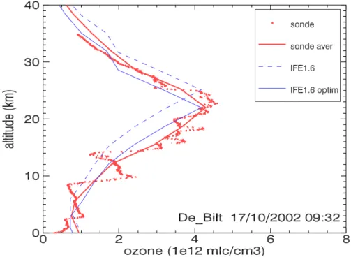
Fig. 8. Example of the too strong gradients above and below the

ozone maximum in optimized IFE ozone profiles.

5 Comparison with sondes using equivalent latitude

A drawback of co-locating satellite profiles with sondes

us-ing distance and time criteria is the low number of data pairs

that is left for comparison, since the number of measurement

stations is limited. A method to increase the number of

co-locating data points in the stratosphere is the use of

equiv-alent latitude as co-location criterion rather than distance.

Equivalent latitude is a useful tool in atmospheric science to

decide whether two points are part of the same large scale air

volume or not (Allen and Nakamura, 2003; Good and Pyle,

2004).

The concept of equivalent latitude exploits the fact that in

the stratosphere, on a time scale of days, air parcels are

trans-ported along lines of constant potential temperature (θ) and

potential vorticity (PV). The altitude above which this is true

is determined by the stability of air; we use a lower border

for θ of

330 K. As a consequence, if two parcels of air on

the same θ-level have the same PV, they are likely to have the

same origin. Potential vorticity has a strong zonal character,

since transport and mixing in longitudinal direction is much

stronger than in latitudinal direction. Since PV increases

from south to north, it is possible to map the PV axis to a

latitude axis from −90

◦

_to

₊₉₀

◦

_{, assigning an ’equivalent}

latitude’ to each PV value. The mapping is such that given a

fixed PV, the equivalent latitude encloses a polar cap starting

at the south pole that covers an area equal to the area

cov-ered by all air parcels with a lower PV. In this way, similar

equivalent latitude means similar PV means similar origin,

and, since on a time scale of days stratospheric ozone

con-centrations are almost constant, it also means similar ozone

concentrations.

In this study, equivalent latitude is used to compare

re-trieved ozone concentrations with sondes that measured the

same air volume; see the illustration in Fig. 9. Profiles of

equivalent latitude as a function of θ and altitude are obtained

for each individual retrieved profile and each sonde launched.

These meteorological profiles are obtained by interpolation

of ECMWF (European Centre for Medium-Range Weather

Forecasts) meteorological fields of θ, PV and geo-potential

height in space and time. For each individual point in one of

the retrieved profiles, the following steps are taken. First, the

θ-level and equivalent latitude at the corresponding altitude

are obtained by interpolation of the meteorological profiles.

Second, for all sondes launched within 24

hours, the

equiv-alent latitude and ozone concentrations are obtained on the

computed θ-level by interpolation of the meteorological

files, respectively averaging the high resolution sonde

pro-file over a small altitude interval. This large time interval

is allowed since even sondes launched at the other side of

the earth might sample the same air as the satellite

instru-ment. Third, only those sonde concentrations are selected

for which the equivalent latitude differs less than 2.5 degrees

form the equivalent latitude of the profile. Note that this is

about

250 km, which is much smaller than the 1000 km

cri-terion used for co-location by distance, but is required to

en-sure that SCIAMACHY and sondes sample the same volume

of air.

Fig. 9. Illustration of co-locating satellite and sonde measurements

using equivalent latitude. IFE profile ’02478 0866 14’ has a tangent

point south-east of Madagascar. At a θ-level of 395 K, the

instru-ment samples air originating from inside the Antarctic polar vortex.

Ozone sondes launched from stations Lauder, Macquarie, and Irene

have sampled the same air at this level, and their measurements can

therefore be compared with the retrieved concentration.

The comparison between retrieved and sonde profiles is

now not on profile-to-profile base, but rather on

point-to-Atmos. Chem. Phys., 0000, 0001–8, 2005

www.atmos-chem-phys.org/acp/0000/0001/

Fig. 8. Example of the too strong gradients above and below the ozone maximum in optimized

IFE ozone profiles.

(25)

ACPD

Full Screen / Esc

EGU

Fig. 9. Illustration of co-locating satellite and sonde measurements using equivalent latitude.

IFE profile “02478 0866 14” has a tangent point south-east of Madagascar. At a θ-level of 395K, the instrument samples air originating from inside the Antarctic polar vortex. Ozone sondes launched from stations Lauder, Macquarie, and Irene have sampled the same air at this level, and their measurements can therefore be compared with the retrieved concentration.

(26)

ACPD

Full Screen / Esc

EGU

Fig. 10. Bias in IFE profiles from comparison with sondes based on equivalent latitude, for

months August to December 2002. Sampled over latitude bands of 20◦ and altitude intervals around the retrieval heights; zonal areas with less than 5 data points are excluded (gray). The dashed line is the ozone maximum according to the sondes.