The discrete-time compensated Kalman filter

THE DISCRETE-TIME COMPENSATED KALMAN FILTER* by

Wing-Hong Lee** Michael Athans**

ABSTRACT

A suboptimal dynamic compensator to be used in conjunction with the ordinary discrete-time Kalman filter is derived. The resultant compensated Kalman filter has the property that steady-state bias estimation errors, resulting from modelling errors, are eliminated. The implementation of the compensated Kalman filter involves the use of accumu-lators in the residual channels in addition to the nominal dynamic model of the stochastic system.

* This research was supported by NASA Langley Research Center under grant NSG-1312.

** Room 35-308, Electronic Systems Laboratory, Department of Elec-trical Engineering and Computer Science, Massachusetts Institute of Technology, Cambridge, MA., 02139, USA

This paper has been submitted for publications to the International Journal on Control.

This is a revised version of a previous paper (ESL-P-748, May 8, 19.771 which contained several algebraic errors. Please destroy the old version.

1. INTRODUCTION

It has been widely recognized that modelling errors can lead to sensitivity problems and even divergence of Kalman-Bucy filter. In cases where the nominal plant parameters used in the filter design are different from the actual plant parameters, the uncompensated

mismatched steady state Kalman-Bucy filter exhibits bias errors. Athans [11 discussed this problem, and presented a brief survey of the various

schemes to reduce filter sensitivity. In particular Ref. [1] introduced the continuous time compensated Kalman filter, a sub-optimal state estimator which can be used to eliminate steady state bias errors when it is used in conjunction with the mismatched

steady state (asymptotic) time-invariant Kalman-Bucy filter. The ap-proach used relies on the utilization of the residual (innovations) process of the mismatched filter to estimate, via a Kalman-Bucy filter, the state estimation errors and subsequent improvements of

the state estimate. The compensated Kalman filter augments the mis-matched steady state Kalman-Bucy filter by the introduction of ad-ditional dynamics and feedforward integral compensation channels.

Satisfactory results of this compensated Kalman filter in a practical design have been reported by Michael and Farrar [2], where it was applied to the estimation and control of critical gas turbine engine variables.

This note follows the same philosophy and development as [l], for the discrete time case. In section 2, we give definitions and

state Kalman-Bucy filter. Section 3 analyzes the errors due to mismatching. Section 4 contains the main contribution which deals with the development of the compensated filter structure and equations. Section 5 contains the discussion of the results.

The elimination of bias errors is accomplished by having accumulators (the analog of integrators) acting upon the residuals. Thus if persistent bias errors exist due to model mismatching, the accumulators provide the

necessary corrections so that the bias errors are removed from the estimates in steady state.

The approach selected was dictated by issues of simplicity of design, namely the use of constant gains in the estimator realization, and the avoid-ance of real time parameter estimation, which requires extensive real time calculations. All calculations of the constant filter gains can be carried out off-line.

-3-2. DEFINITIONS AND ASSUMPTIONS

Only modelling errors in plant parameters will be considered throughout this paper. We believe that this is often the case in practice. _{When there are errors in the statistical parameters of the} underlying random processes, a different approach is required and the results are more complicated.

2.1 Actual Plant Description

We assume that the actual plant is an n-th order linear time-invariant, stochastic dynamical system with state vector x(t)S Rn, constant input vector u S Rm and noisy measurement vector z(t) c Rr described by

(State Equation) x(t+l) = A x(t) + B u + i(t) (1)

(Measurement Equation) _{z(t) = C x(t) + @(t) (2)}

where A, B, C are respectively nxn, nxm, rxn constant matrices-. The plant noise i(t) and the measurement noise @(t) are white Gaussian stationary processes with the following statistics, which are assumed to be known to the designer.

E(~(t))= O for all t (3)

~E~{-

ts)i'(t )}- -dt for all s,t (4)

E(e(t))= O for all t (5)

E{8(s)8'(t)} = 8.6 for all s,t (6)

where cst denotes the Kronecker delta, and ~, the plant noise

intensity matrix, is a constant nxn positive semi-definite symmetric matrix, while 0, the measurement noise intensity matrix is a

constant rxr positive definite symmetric matrix. Moreover, i(t) and

8(s)

are assumed to be uncorrelated for all s, t, i.e.

E{_(t)e'(s)} = O (7)

It is further assumed that (with t_o -* + )

E{x(t )} ₀ = O (8)

2.2 Model Description

The actual plant dynamics are defined by the values of the three constant matrices A, B, C in equations (1) and (2), and

the noise statistics defined in equations (3)-(8). We shall assume that the actual values of A, B and C are not known exactly to the designer. Rather, nominal values A , B n, C are available to the

designer in addition to perfect knowledge of the noise statistics, and the value of the constant input vector u. Thus as far as the designer

is concerned, the model is given by

x(t+l) = A x(t) + B u + i(t) (9)

z(t) = C x(t) + 8(t) (10)

-5-For later development, define the following parameter error matrices:

AA - A- A

(11)

AB - B (12)

Ac

c-

C-

(13)

2.3 Further Assumptions

We limit the discussions to constant gain filters, as in [11, since they represent one of the most practical uses of Kalman-Bucy filters from the application viewpoint, and they can readily

lead into steady state error and stability analysiso The following assumptions are necessary for the derivation of the results.

1.

£A,B]

and (A ,B

]

are controllable pairs.

2. [A,C] and [A ,Cn] are observable pairs.

1/2

,1/2

3. [A,/ ] and [A ,1 ] are controllable pairs. 4. Both A and A are strictly stable matrices, i-.e

all of their eigenvalues lie within the unit

circle. This also implies that (A-I)}1 and (A - I)1 exist. These assumptions are indeed necessary for the rigorous development of a unique, stable, steady state Kalman-Bucy filter.

Let us suppose that the designer constructs the NMSSKBF on the basis of the nominal parameter values available to him and the as-sumed known statistical parameters. Then the state estimate of x(t); x (t)e R , generated by such a filter, is given by the following -n

mismatched filter dynamics.

x Ct+l t) = A £ (t) + B u C14al -T n-- -- -- -x (t+l) = -x (t+llt) +G r Ct+l), x Ct_o) =O (4b). --n --n -n-n - 0 -r Ct) = zCtl - Cx Ct t-'1. CiS L n --n-n

where G is a constant nxr filter gain matrix given by -n

G = Z C' (O + C C') (16)

-n -n -n - ,-n -n

and Z is the nxn constant, symmetric, positive definite solution -n

of the algebraic matrix Riccati equation [3]

A E A' - A E C'(C 7 C' + O) C Z A' + B = = (17) -n-n-n -I --nn -n--n -- - r--n

-The block diagram of the NMSSKBF is shown in Figure 1.

The existence of G and Z are guaranteed by our assumptions. Also it is well known that the closed-loop filter matrix

[A - A G C ] = [A - A 7 C' (O + C 7 C ) C ] (18) -n -- n-n -n -n--n --- -n--n n

$4 a E I, 4) -. 0° 4-1*

_¢

_i

¢U + , E-* CP 0 c

severe inaccuracies arise due to the fact that the nominal plant matrices A , B , C are used rather than the actual (but unknown)

~-n

n--n

matrices At B, C. These effects are particularly bothersome because bias errors in the estimates exist. It is instructive to isolate

these errors, because the structure of the equation suggests that compensation techniques can be used.

3.1 Estimation Errors and.their Dynamics

Define the state estimation error x (t) induced by the NMSSKBF by

x (t) (t) - x t-l) (19)

From equations (1), (2), (14), (15), and (19), one can readily deduce that the state estimate error x (t) satisfies the stochastic difference equation

x (t+l) = A x(t) + B u + i(t) - (A x (t) + B u) (20)

-9-x (t+l) = [A -A G C ]x (t) + 5(t)-A G i(t) + AA x(t)-A G AC x(t)

-n -n -n-n-n -n -n-T- --

-+-AB u (21)

3.2 Mean State Estimation Error

Equation :C21) readily allows one to deduce the effects of model mismatching upon the estimation errors; bias effects are introduced. To compute these, one simply takes expected values in equation (21). We remark that the expectations are not conditional ones, since the

filter structure has been fixed. Thus

E{X (t+l)} = [A -A G C ]E{x (t)} + AA E x(t)}

-n n n ---- l -n

(22) -A G AC E{x(t)} + AB u

But' from equation (1),

E{x (t+l)} = A E{x(t)} + B u (23)

This yields, in view of equation (C8, a non-zero mean state, ie,, t

E{(t)} =A B u # 0 (24)

Tt=_o

Thus, if some or all of AA, AB, and AC are non-zero, then one can readily conclude from (22) that bias errors exist. Note that the effect of the constant input u accentuates these errors, even for stable system. From equations (22) and (24),

t-t

E{x (t)} = [A -A G C

i

E{X (t

)}

-n -n-n-

(25)

t s

+ E [AA G C I ts [A A AG Ac] E AS B +AB}

S=to T =to

Noting that, in view of equations (8) and (14),

E{x (to)} = E{x(to)} - {x (t0)} = (26)

equation (25) becomes

s

t t-s

E{X(t

)}

E [A -AG C

I

{[AA-A G

Ac]

[ ASTB]+AB}u

st0 0 (27)

This is in general non-vanishing, and cannot be evaluated since A, B. C, & AB, AC are not known exactly. In particular, as t gets large, the mean steady state estimation errors are approached,

lim E{x(t)} = -[A-I] B u (28)

to00

lim E{x (t)} = - A - I] [AA-A G AC] [A-I] B-AB}u (29)

_- 1 -n _--- _ TT -- -- ..

Both of these are non-zero. Therefore, in the mismatched case, there exists a non-zero mean steady-state estimation error. Again, due to incomplete information, one cannot compute this mean steady-state estimate error so as to add it to the NMSSKBF estimate x (t) to arrive_--n

at unbiased estimates.

3.3 Discussion

The above development indicates that the NMSSKBF should not be used without further modification. It necessitates the use of com-pensation by a suboptimal estimator, because the truly optimal filter

(that estimates the unknown elements of A, B and C) is an infinite dimensional one [3]. The degree of suboptimality has to be related

to the extra dynamics that are required to improve the performance of the nominal mismatched Kalman-Bucy filter.

The next section presents a compensation technique, which is similar to [1]. The central idea is that it augments the NMSSKBF by additional filter dynamics and tries to extract further

informa-tion from the residual (innovainforma-tion) processes. It has the merits that all gains can be pre-computed, and it avoids the complexity of non-linear estimation (or the extended Kalman filter algorithm) which

is not always guaranteed to work properly [3]. Moreover, it compen-sates the biased mean steady state estimate error without sacrificing the accuracy of the state estimate, i.e. increase of RMS errors, which is very often the case when other techniques are used, e.g., increased

4. 'THE DEVELOPMENT OF THE DYNAMIC 'FILTER COMPENSATOR

First recall the dynamic equations of the state estimation error x (t), and the residual process r (t) (equations

(21), (15)).

x (t+l) = [A i-A G C.]x (t) + r(t)-A G 8(t) + AA x(t)-A G AC x(t)

-n -n -n -- I-T ---

n----+-AB u (30)

=_(t) = z(t) - C

x

Ctlt-l) (31)

Using equations (1),(2) and (19), equation (31) can be written as

r (t) = C x (t) + AC x(t) + 8(t) (32)

dn -n -n

Note that the residual process r (t) is linear in the state estimation -n

error x (t). It is reasonable to attempt using equation (32) as a "measurement equation" to obtain an estimate of x (t), the state estimation error. However, the existence of the unknown matrices, AA, AB and AC in equations (30) and (32) prohibits us from solving this as a linear estimation problem. Thus certain approximations have to he made, In what follows, it is shown how one can form such a linear estima-tion problem, by making approximaestima-tions with. reasonable physical inter-pretation.

-13-4.1 Philosophy

Define the time sequences w(t)s R and v(t)s Rr as follows:

w(t) = AA x(t) + AB u (33)

v(t) =

AC

x(t) (34)

Thus equations (30) and (321 reduce

to-x (t+l) = [A-A G C ]to-x (t) + w(t)-A G v(t) + L(t)-A G @(t)

-n -n -n -n--n - - -n- -

--(35)

r (t) = C x (t) + v(t) + 0(t) (36)

-n -n -n

Now it is apparent that equations (35) and (36) form a linear esti-mation problem, with correlated plant and measurement noise, provided that w(t) and v(t) satisfy linear equations. So the next step is to develop simple linear equations for w(t) and v(t). If one is- pri-marily interested in the development of a steady-state constant gain filter, one can proceed as follows.

From equations (28) and (33), we can deduce that

lim E{w(t)} = [AB + AA(I-A)- B]u = unknown constant (37) Also

Equation (37) implies that w(t) must have a nonzero (but unknown) mean steady state, while equation (38) indicates that it must contain a zero mean driving noise term. Both of these objectives can be satisfied if one selects the dynamics of w(t) to be of the form

w(t+l) - w(t) = (t); w(t 0) O0 (39)

where Y(t) is a zero mean, white, Gaussian stationary process, i.e.

E{I(t)} = O (40)

E{Y(t)Y' (T)} := at (41)

r

=

r'

> 0 (42)

Similarly, for v(t), from equations (28) and (34), one can see that

lim E{v(t)} - A AC(A-I) B u = unknown constant (43)

and

v(t+l) - v(t) =AC-CAI)xC(t) + B u] + AC i(t) (44)

This leads are to select the dynamics of v(t) by the equation

v(t+l) - v(t) = k(t); v(t₀ ) O (45)

where X(t) is a white, Gaussian, stationary noise process with statistics

E{X(t)} = 0 (46)

E{X(t)' (T)} = At _t'T (47)

A =

A'

> 0

We remark that if AA is known (or can be estimated on the basis of physical considerations) one should select

YCt)

--= A (t) (48)

and set

r

P= AA E AA (49)

Similarly, if AC is known (or can be estimated) one should select

X(t) = AC i(t) (50)

and set

A = AC E AC' (51)

In view of equations (48) and (50), or physical reasoning, one should consider y(t) and X(t) as two correlated processes, i.e.

E{I(t)X' (z)

}

= X t (52)

Indeed if both AA and AC are known or can be estimated, one should set

Also _(t) should be correlated with y(t), and X(t). Let

E{i(t)y' (Q)}

-YY

a

'(54)

tT

}

E{E(t)X'(c)1 = (55)

In particular

Q2 = LAA' (56)

if AA is known (or can be estimated), and

Q2 = nAC' (57)

if AC is known (or can be estimated).

The above development allows one, by making certain ap,

proximations, to replace equations (30) and (32) by a linear estimation problem with plant dynamics_ gi.ven by

(t+l) A-A G C I -A ·G x (t)- I 0 0 -AG W(t) r n1 -n-n-n -- -n-n

w(t+l)

0O

I

_

w(t)

O I 0 0

XY(t)

(58)

_ v(tel) O I v(t) 0 0 I O _ (t) 8(t) ~(t+l) F ~(t) D_

--

-r (t) [C _

-n W

+59)--H v (t)

Thus a Kalman-Bucy filter can be designed to generate estimates of x (t), w(t), and v(t), denoted respectively by, x (t), w(t), and v(t), based on past measurements of r (T), t <

r

< t.

Recalling that (see equation (19))

x(t) = x _-n (tt-l) +(t) _-n (60)

it is clear that an improved predicted esthilate. iCtl t-l, and updated estimate xCt) of xCt2 can be constructed by.

xCtIt-1) =- Ctit-l) + x CtIt-L (C61a4

xtl-= x Ctlt-1-3--+ th-1 ¢tL Ctl

-n -1

4.2 Details of Constructing the Compensated Filter

Using a steady state Kalman-Bucy filter, the estimates. x (t),

-n ,

w(t) and v(t) are generated via the following equations

x(t+ljt) = [A -A G C x (.t) + wtCtl - A G vCt) -A G 0(9( + HS'Z -- -1n -n -n1--n--1 -n n- -- - - -[r It) -C x (tlt-1)-(t-1)] (62a) -n1 -n-n x (t+l) = x (t+llt) + L [r (t+l) C - (t)] (62b) w(t+l) = w(t) + L Cr (t+l) - C x (t+lIt) - v(t)] (63) (t+l) (t) + [r (t+l) L -C x (t+lt) -(t)] (64) (t+l) =(t) + L Er (t+) -C

i

(t+lt) - Ow(t)l (64) -v -

--where L, L , L are respectively nxr, nxr and rxr constant

matrices (steady state filter gains), which will be defined below. The initial conditions that one might use are

x (t = (65)

w(t0) = 0 (66)

v(tO) = O (67)

They are chosen because one can view AA, AB, AC as random matrices with zero means, the nominal values A , B , C used by

the designer represent the a priori mean values of A, B and C, respectively.

Now referring back to equations C581 and (59), define for notational convenience the matrices

w

~

0

M = (68)

_'

?r %1 0

s' ' A O

=-x

-yX

-0

0

0

°

N ° (69) 0 0

-19-Then M plays the role of the composite plant white noise (+J(t))

intensity matrix, and N yields the correlation between the composite plant white noise 9_(t) and the measurement white noise 8(t).

Let S denote the steady state predicted error covariance matrix associated with the estimation problem defined by equations C58Y and (59). Then S is a symmetric at -least semi-positive definite matrix. In addition,- it is the positive semi-definite matrix solution to the algebraic Riccati equation -Ctake e.g. the dual in [5].

S = [F - D N E H] [S - S H' (O + H S H') H S] [F - D N ]

+ D[M -.N _ 1N'ID' (70)

Onecan then compute the filter gain matrices L , L and L that appear in (62)-(64) by

L = H' ( + H S H') 1 (71)

4.3 Simplification

The realization of Section 4.2 can be considerably simpliified. Define the compensated residual process r(t) by

From equation (61) we deduce that

r(t) = z(t) - C x (tlt-ll - C x (tit-l - Oct-ll (73) _

_ -n- n-n --

-Then from equation (15), this becomes

r(t) = r (t) - C x (tit-le - OCt-ll (74)

Equations (61), (62), (14) and (74) yield

x(t+llt) = x (t+llt) + x (t+llt) (75) = A x (tIt-l) + B u + A G r (t) -n-n - -n--n + (A -A G C )x (t) + w(t) - A G 9(t) n -n-n-n --n -n-- A G e(e + H S H') r(t) = A x(t) + B u + w(t) + [(A G - A G C L - A G L ) - A G ( + H S H') ir(t) -n-n 11-n-n-n--x -n--n- - --

From equation (71), it is easy to see that

C L + L = HSH' (O + H S H')

-n-x v

-After a little algebra, it can be shown that the last term in equation (75) vanishes for all t. That is, equation (75) reduces to

x(t+lt) -= A x(t) + B u + w(t) (76a)

Thus the compensated state estimate x(t+l) is given by

x(t+1) = x (t+l

It)

+ x (t+l) (76b)

= x (t+ljt) + (t+lt) + L r(t+l)

- x(t+ljt) + L r(t+l) (76e)

In addition, equations (63) and (64) become

w(t+l) = Q(t) + L r(t+l) (77)

~~-w-

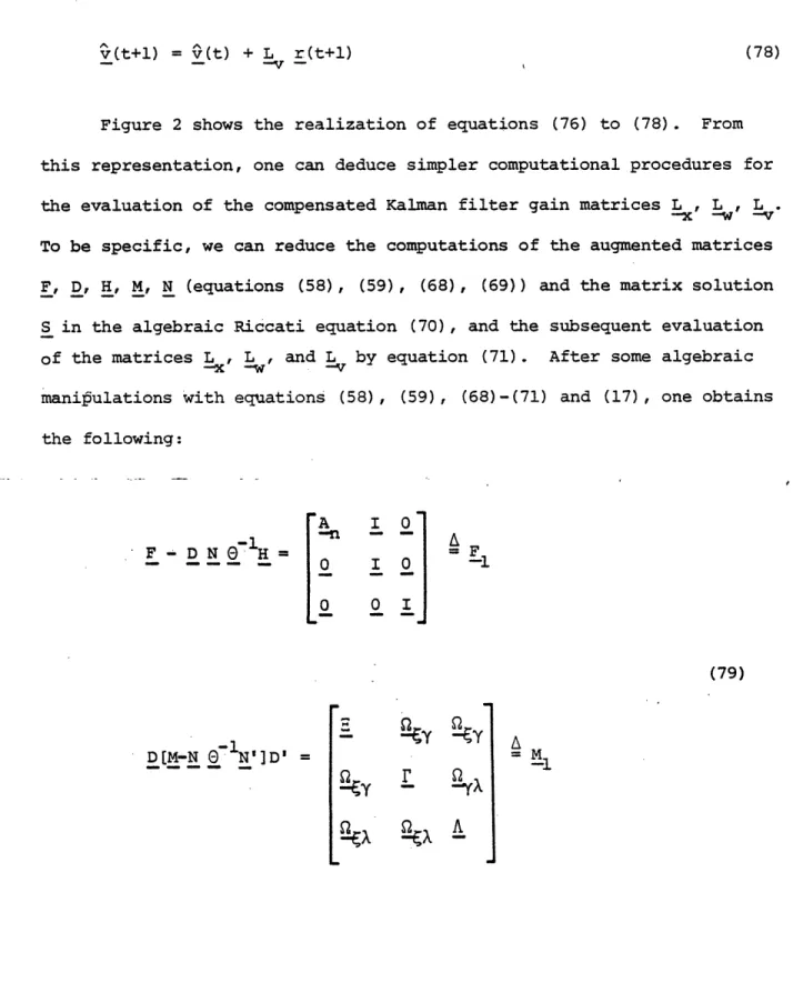
-21-v(t+l) = v(t) + L r(t+l) (78)

Figure 2 shows the realization of equations (76) to (78). From this representation, one can deduce simpler computational procedures for the evaluation of the compensated Kalman filter gain matrices L , L , L

-x - --V

To be specific, we can reduce the computations of the augmented matrices F, D, H, M, N (equations (58), (59), (68), (69)) and the matrix solution S in the algebraic Riccati equation (70), and the subsequent evaluation of the matrices L , L , and L by equation (71). After some algebraic

-x -w

-manipulations with equations (58), (59), (68)-(71) and (17), one obtains the following: A I 0 F -D N dlH F I A (79) D[M-N e'NI]D' = A-|_ - ¥£ ¥A

E

_

_E

L f J

tEt

_U..,

I~~wS

,4-

~~~~~~~~~~~~~~4a

E

_~II

_<31( +

_t

. 1 I<I 8 4J + _ + so z' N4 _co k~~~~~~~~~~~~~~~~~~~~~~~~~~~~~~~~~~U ___ __ __ *u cro~~~~~~~~~~~~~~~~~~ *p MgN Z co

and equations (70), (71) become S -F[S- S H' (E + H S H') H S]F_ + _ (80) L L =-S- '(R + S H') (81 4.4 Discussion 4.4 Discussion

The structure of the discrete-time compensated Kalman filter, illustrated in Figure 2, has certain appealing physical aspects. The major structural difference between the uncompensated Kalman filter of Figure 1 and of the compensated one of Figure 2, hinges upon the addition of distinct accumulator loops driven, through appropriate gains, by the compensated residual vector r(t+l). Note that an

accumulator is the discrete time analog of an integrator in the continuous time case. In the absence of any accumulators, the residual vector of the the uncompensated Kalman filter would exhibit bias errors. In the com-pensated filter these residual bias errors are accumulated (integratedY with appropriate weightings (the gain matrices L and L in Figure 2). in two different ways. The accumulator that generates the sequence '(t) corrects for bias errors in the predict cycle, to compensate for the errors modelled by the matrices AA and AB. This makes sense, because w(t) was defined by Eq. (33) in terms of AA and AB. The accumulator that generates the sequence v(t) corrects for bias errors in the

residuals due to modelling errors 6C in the measurement equation;

if AC = 0, the accumulator channel that generates "(t) would be absent. One can then think of Q(t) as being a crude estimate of constant but unknown disturbances that are additive to the state equations, and of v(t) as a crude estimate of constant but unknown bias errors in the measurement equation.

The improved estimate x(t+l) generated by the compensated Kalman filter (Figure 2) is still instantanously influenced by the compensated instantaneous residual r(t+l) through the feedforward gain L . The

nominal dynamics A , B , C are still being utilized and bias corrections via Q(t) influence the predicted compensated estimate _(t+llt) and

hence the residual.

Obviously the transient performance of the estimation errors of the compensated Kalman filter would hinge upon the numerical values of the three gain matrices L , L , and L . These in time would not only de-pend upon the nominal parameters, but upon the way the intensity matrices of the white noise sequences yCt) - see eq. (39) - and _(t) - see eq.

(45) - are selected. It is the authors'opinion that the suggested guidelines for the covariance selection are reasonable, since for most practical problems the designer has a reasonable idea of the worst

possible modelling errors, exhibited in AA, AB, and AC, from the nominal parameters. It is important to stress that the white noise intensity matrices r and A not only depend upon the modelling errors, but also upon the intensity matrix , of the original plant noise E(3~f shown by. eqs. t49) and (51). Furthermore, ytL and alCt_ are correlated according to eqs. (52) to C57). Thus, the guesswork on the part of the designer ias minimized.

-25-5. FURTHER SIMPLIFICATIONS IN PRACTICAL DESIGNS

At first glance, the compensated Kalman filter might seem some-what complicated than that of the NMSSKBF alone. We remark that the complexity is directly related to the dimensionality of the two

auxiliary vectors v(t) and w(t). However, in most cases of practical interest, canonical representations can be used to arrive at the smallest number of additional accumulators in the realization of the compensated Kalman filter.

5.1 A Single Input Single Output Example

To illustrate these implications consider the design of the compensated Kalman filter in the case of linear, time-invariant, stable single input single output plants. Suppose that the actual plant is characterized by its transfer function

n-i n-2

c z

+

z

+...O2z

+c

G(z) = . nI2 (82)

n n-l

z +az ++az al

Then there are at most 2n unknowns (the a.'s and c 's) in the plant description.

Let a . and ci-, i=l,...,n,denote the nominal values of the a. and ci , respectively. Then the standard controllable representation for the actual plant (equation (82)) is

o 1 ... 0 x(t+l) = 0 0 1 0 ... 0 x(t) + O u(t) + i(t) 0 (83) -a1 -a ... -a B A z(t) = [c c2 ... c ]x(t) + 0(t) (84) C

and the nominal values of A, B, C are (in the same representation)

-~---n _{0 1 0 ...} -n ₀ A = 0 0 1 ... 0 (85) aln -a .... .. -a_ 2n 2 n 0 B = 0 (86) -n

(

c Ic. ... c

J

(87) -n- n n nn

-27-Thus

AA

C=

((n-1) rows)

(88)

·

a' AB = 0 (89) AC = 6c' (90) where

6a' = [alaln, a ... 2-a 2n, , an-a nn] (91)

3c' = [Cl-cln c2-C2n, .. C , n-cnn] (92)

Examine the way the vector wCtI is defined Cequat ion (33)L, Since AB = 0, w(t) is given by

w(t) = AA x(t) = (93)

_-a-x(t)

which means that although w(t) is an nxl vector, it really contains only one uncertain parameter, namely the scalar w n(t),

v(t) in this case is also a scalar

v(t) = dc'x(t) (95)

Following then the procedures described in Section 4, one can see that the'scalars w (t) and v(t) should be-modelled as

(t+) n(t) = w (t+l) - v (t) = A (t) (96) v(t+l) - V(t) = X(t) (97) with E{yn(t)} = 0 (98) E{X(t)} = 0 (99) and E{yn(t)yn(T)} =

r

nndt (100) E{X (t)X(T) } = tAt ₍₁₀₁₎ E{y (t) X (T)} = X tT (102) E{E(t)Yn(T)} = i3 ₍₁₀₃₎

E

(t)

n (l)} X 1YntT E{((t)x(T)} }

X

tr

(104)

-29-Ideally, one selects

r

=6a' a

da

(105) nn A = dc' E c - (106) x =& da'" . c, (107) n

a

= = 6 a (108) = ( c (109)

In practice, since 6a and 6c are not known one should use their worst possible values in equations (105)-(109) to determine the covariances.

Under these conditions, the equations of the compensated Kalman filter become (see equations (76)-(78))

0 1 x(t+l) A x(t) + B u + L r(t+l)+ (110) w (tW

i

^ A w (t+1) w n(t) + L r(t+l) (111) n n wn v(t+l) = V(t) + L r(t+l) (112)

with

r(t) = z(t) - C xCt It-ll - t-l)) (113)

where

a) L H is a constant nxl gain vector;

b) L is a constant scalar gain; wn

c) Lv is a constant scalar gain.

5.2 Extension to Multi-Input Multi-Output Systems

The above procedures can be easily extended to the multi-input multi-output systems. We outline the step by step procedure that should be followed.

Step 1: Examine the structure of the nxn matrix AA for arbitrary variations of the actual and nominal plant parameters. Let p, O<p<n, denote the number of non-zero rows of AA. Define an nxp matrix P according to the following rule. Let j=1,2,..., P index the columns of P.

(a). Let i=l, j=1

(b). If the i-th row of AA is nonzero, set the j-th column of P equal to e_i (the natural basis vector in Rn), set j=j+l, and go to (c). If the i-th row of AA is zero, go to (c). (c). If i=n stop; otherwise set i=i+l and go to (b).

-31-Example: Suppose AA has the structure (where x denotes a nonzero element)

'AA= 0 x 0 x 0

x 0

x x x 0

Then p=2, and the 4x2 P matrix is given by

0 0 1 0 0 O 01

Step 2: Examine the structure of the rxn matrix AC for arbitrary variations of the actual and nominal plant parameters. Let q,

O<q r, denote the number of non-zero rows of AC. Define an rxq matrix

2

according to the following rule. Let k=l1,2,...,q index

the columns of Qo (a). Let i=l, k=l

(b). If the i-th row of AC is non-zero, set the k-th column of

2

equal to e. (the natural basic vector in Rr), set k=k+l, and go to (c). If the i-th row of AC is zero, go to (c).

(Cc). If i=r, stop; otherwise, set i=i+l and go to (b).

Exanple:- Suppose that AC has the following structure

x x 0 0 x 0 O 0 0 0

Then q=l and the Q matrix is given by

Ste 3 Let (t such that

Step 3: Let w(t) e , ₁(t) s , such that

w_ (t+l) -wl(t) = yl(t) (114)

with

E [ ₁(t)] = o (115)

Make the identification (116)

-33-w(t) P w(t) (117)

y(t) P'y(t) (118)

*r 1 = P'FI P (119)

-1 _ _ _

Step 4: Let vl(t) e Rq, Xl(t) Rq such that

v(t+l) - v(t) = Al(t) (120)

with

Exl (t)] = (121)

E [ l (t) '(T) ] = A 6 t (122)

Make the identification

v(t) = 2 vl (t) (123)

kl(t) = ;'X(t) (124)

A1 g V (125)

Step 5: Assume that i(t), l(t) and Xl(t) are pairwise correlated.

E[ (t)l(l)] = yt= (126) E[ (t)XL(T)] = ~ (127) E 0 X 6 (128) 1l

~

Make the identification

i =l i P (129)

ic\, 1~ (130)

-Y2 =P'-, (131)

5.3 Reduced Dimension Compensated Kalman Filter: Summary

of Equations

The following equations are obtained by substitution of equations (114) through (131) into (76) to (78).

Filter Equations

x(t+l1t). = A

£(Ct)

+ B u + P w Ctl (132a)

x(.t+lIt+12 = xCt+lit + irlr Ct+ ( C1 32b)

_l (t+l) = v (t + L lrl(t+l) 33al

-1( -11 t + L-lit+

rlCt+l) = zCt+l1 - C x(-t+ltI - Q v(ct) 1341

Filter Gain Equations

The filter gain matrices L (nxr), L (pxr, and L Cqxrl are given

-xl w 'rl-v

by

L |1 =Y a', + H Y I- (135)

-35-where Y is the unique (symmetric) positive definite solution of the (n+p+q)-th order algebraic matrix Riccati equation

Y F2Y - Y H'(e + H Y H) -HY]F2 M (136)

--2 - 1 - -1- =-1 -2

:F-2' HL' M2 are respectively (n+p+q)x(n+p+q), rx(n+p+q), (n+p+q)x (n+p4q) constant matrices given by

A P O -2 O I 0O (137) H= [C 0 q] (138)

-f

-X

X

₁ M2 (139) 5.4Y Ds s-l P X1 _l -1 5.4 Discussion

The compensated Kalman filter equations presented in Section 5.3 are the recommended ones for practical design. The additional

workload associated with the computation of the P and Q matrices is justified in terms of the simplification that results in specific problems.

From a technical viewpoint the essential difference between the filters of Section 4.3 and 5.3 is that in the latter case the compensated Kalman filter can be shown to possess all the requisite controllability and observability conditions which are necessary for the existance of a unique positive definite solution to the al-gebraic matrix Riccati equation and the guaranteed stability of the resultant filter. It also pinpoints the additional number

(p+q) of accumulators required to stabilize the uncompensated filter. The only "guesswork" required by the designer is the selection of the intensity matrices

r

(pxp) and A (qxq) and the correlation covariance matrices ¥ (nxp), i (nxq) and l (pxq). All of them scale with the intensity matrix I of the plant noise i(t). This is evident from equations (49), (51), (53)-(55), (119), and

(125)-(128), from which we obtain

rV = P'AA -AA'P (140)

-3-A=

'SAC _

Ac'A

(141) A- 2 = AA'P (142) XX

=

E AC'j (143) -

P'lAA

- AC'} (144)

-37-Since g is assumed known, and P and Q are readily evaluated, the selection of l

A, Q

and n only involves the use

of judicious estimates for iA and AC by the designer. As

remarked before, these estimates can be usually found from a worst case analysis, i.e., the worst probable deviation of each parameter

from its assumed nominal value. Of course, there is still an ele-ment of judicious judgeele-ment to be made; at least in this design the "guesswork" can be related to the degree of worst deviation of the nominal plant from the actual one.

A method for compensating the mismatched constant gain discrete time Kalman filter has been presented. The resultant compensated Kalman filter is time invariant, and the gains are all computed off-line, with some

added complexity to the estimator. The compensation consists of the intro-duction of feed-forward accumulating (integrating) channels between the residual process and the uncompensated mismatched filter.

The compensated Kalman filter has the property that bias errors in the state estimates are eliminated asymptotically. More complex algorithms have to be used if unbiased estimates are required for all t.

-39-REFERENCES

[1] M. Athans, "The Compensated Kalman Filter," Proc. Symposium on Nonlinear Estimation, University of California at San Diego, September 1971.

[2] G.J. Michael, F.A. Farrar, "Estimation and Control of Critical Gas Turbine Engine Variables," ASME paper, 76-WA/Aut-12, 1976. (3] A.H. Jazwinski, Stochastic Processes and Filtering Theory, N.Y.

Academic Press, 1970.

[4] M. Athans, "The Discrete Time Linear-Quadratic-Gaussian Stochastic Control Problem", Annuals of Economic and Social Measurement, Vol. 1, No. 4, 1972.

(5] P. Dorato and A.H. Levis, "Optimal Linear Regulators: The Discrete Time Case" IEEE Trans. on Auto. Control, Vol. AC-16, No. 6,