Modélisation inverse des flux de CO2 en Amazonie

(1)

HAL Id: tel-01697602

https://tel.archives-ouvertes.fr/tel-01697602

Submitted on 31 Jan 2018

HAL is a multi-disciplinary open access archive for the deposit and dissemination of sci-entific research documents, whether they are pub-lished or not. The documents may come from teaching and research institutions in France or abroad, or from public or private research centers.

L’archive ouverte pluridisciplinaire HAL, est destinée au dépôt et à la diffusion de documents scientifiques de niveau recherche, publiés ou non, émanant des établissements d’enseignement et de recherche français ou étrangers, des laboratoires publics ou privés.

To cite this version:

Luis Molina Carpio. Modélisation inverse des flux de CO2 en Amazonie. Océan, Atmosphère. Uni-versité Paris Saclay (COmUE), 2017. Français. �NNT : 2017SACLV040�. �tel-01697602�

(2)

NNT : 2017SACLV040

M

ODÉLISATION

I

NVERSE DES

F

LUX DE

CO

₂

EN

A

MAZONIE

Thèse de doctorat

de l’Université Paris-Saclay

préparée à l’Université de Versailles Saint-Quentin-en-Yvelines

Ecole doctorale N

◦

₁₂₉

Sciences de l’Environnment en Ile-de-France (SEIF)

Spécialité de doctorat: Météorologie, océanographie et physique de

l’environnement

Thèse présenté et soutenue à Gif sur Yvette, le 24 octobre 2017, par

M. L

UIS

MOLINA CARPIO

Composition du Jury :

M. MATTHIEUROY-BARMAN, LSCE, PRÉSIDENT

M. EMANUELGLOOR, UNIVERSITY OFLEEDS, RAPPORTEUR M. WOUTERPETERS, UNIVERSITY OF WAGENINGEN, RAPPORTEUR MME. KARLALONGO, USRA/GESTAR, EXAMINATEUR

M. BRUNO GUILLAUME, ARIA TECHNOLOGIES, EXAMINATEUR M. PHILIPPECIAIS, LSCE, DIRECTEUR DE THÈSE

(3)

(4)

Titre : Modélisation inverse des flux de CO2 en Amazonie

Keywords : Amazonie, flux CO2biogénique, inversion atmosphérique, échelle régionale

Résumé : Une meilleure connaissance des variations saisonnières et interannuelles du cycle du car-bone en Amazonie est essentielle afin de comprendre le rôle de cet écosystème dans le changement climatique. La modélisation atmosphérique inverse est un outil puissant pour estimer ces variations, en exploitant l’information sur la distribution spatiale et temporelle des flux de CO2 en surface contenue

dans des observations de CO2 atmosphériques. Néanmoins, la confiance en les estimations des flux en

Amazonie obtenues à partir des systèmes d’inversion mondiale est faible du fait du manque d’observations dans cette région.

Dans ce contexte, j’ai d’abord analysé en détail les estimations de l’échange net de CO2 entre la

biosphère et l’atmosphère (NEE) générées par deux inversions mondiales pour la période 2002 – 2010. Ces deux inversions ont assimilé des données provenant du réseau mondial d’observation du CO2

atmo-sphérique hors de l’Amérique du Sud, et une d’elles a assimilé des observations de quatre stations de surface en Amazonie, qui n’ont jamais été exploitées dans les études d’inversion précédentes. J’ai montré que dans une inversion mondiale les observations de stations loin d’Amazonie et les observations locales contrôlaient la NEE. Pourtant, les résultats ont révélé des structures à très grande échelle peu réalistes. L’analyse a confirmé le manque de stations en Amazonie pour fournir des estimations fiables, et les limites des systèmes d’inversion mondiale avec des modèles à très basse résolution.

J’ai donc ensuite évalué l’apport de l’utilisation du modèle atmosphérique régional BRAMS, par rap-port à celle du système mondial de prévision météorologique ECMWF, pour le forçage météorologique du modèle de transport atmosphérique CHIMERE simulant le CO2 en Amérique du Sud à haute

résolu-tion (∼35 km). J’ai simulé le CO2 avec les deux modèles de transport—BRAMS et

CHIMERE-ECMWF. J’ai évalué ces simulations avec des profils verticaux de mesures aéroportées, en analysant les mesures individuelles et les gradients horizontaux de CO2 calculés entre paires de stations dans le sens

du vent, à différentes altitudes ou intégrés sur la verticale. Les deux modèles de transport ont simulé les observations de CO2 avec une performance similaire, mais j’ai trouvé une importante incertitude sur les

modèles de transport. Les mesures individuelles et les gradients horizontaux ont été surtout sensibles à la NEE, mais aussi, pendant la saison sèche, aux émissions des feux de biomasse (EFIRE). J’ai trouvé que

l’assimilation des gradients horizontaux était plus approprié pour les inversions que celle des mesures individuelles, étant donné que les premiers ont été moins sensibles au signal associé aux flux hors de l’Amérique du Sud et à l’incertitude sur le modèle de transport en altitude.

Finalement, j’ai développé deux systèmes d’inversion régionale pour l’Amérique du Sud tropicale avec les deux modèles de transport, et j’ai lancé des inversions avec quatre types de vecteurs d’observation: de mesures individuelles et gradients horizontaux sur cinq niveaux verticaux, à la surface, ou de gradients

(5)

inversions assimilant des gradients horizontaux ont séparé mieux les signaux de NEE et EFIRE. Cependant,

les grandes incertitudes sur les flux inversés ont réduit la confiance en ces estimations. Par conséquent, si mon étude n’a pas amélioré la connaissance des variations saisonnières et interannuelles de la NEE en Amazonie, elle a montré les besoins d’amélioration de la modélisation du transport dans la région et de la stratégie de modélisation inverse, du moins à travers une définition du vecteur d’observation appro-priée qui prenne en compte les caractéristiques des données disponibles, et les limitations des modèles de transport actuels.

(6)

Title : Inverse modeling of CO2fluxes in Amazonia

Keywords : Amazonia, net ecosystem exchange, atmospheric inversion, regional scale

Abstract : A better knowledge of the seasonal and inter-annual variations of the Amazon carbon cycle is critical to understand the influence of this terrestrial ecosystem on climate change. Atmospheric inverse modeling is a powerful tool to estimate these variations by extracting the information on the spatio-temporal patterns of surface CO2 fluxes contained in observations of atmospheric CO2. However,

the confidence in the Amazon flux estimates obtained from global inversion frameworks is low, given the scarcity of observations in this region.

In this context, I started by analyzing in detail the Amazon net ecosystem exchange (NEE) inferred with two global inversions over the period 2002 – 2010. Both inversions assimilated data from the global observation network outside Amazonia, and one of them also assimilated data from four stations in Amazonia that had not been used in previous inversion efforts. I demonstrated that in a global inversion the observations from sites distant from Amazonia, as well as local observations, controlled the NEE inferred through the inversion. The inferred fluxes revealed large-scale structures likely not consistent with the actual NEE in Amazonia. This analysis confirmed the lack of observation sites in Amazonia to provide reliable flux estimates, and exposed the limitations of global frameworks, using low-resolution models to quantify regional fluxes. This limitations justified developing a regional approach.

Then I evaluated the benefit of the regional atmospheric model BRAMS, relative to the global forecast system ECMWF, when both models provided the meteorological fields to drive the atmospheric transport model CHIMERE to simulate CO2 transport in tropical South America at high resolution (∼35 km). I

simulated the CO2distribution with both transport models—CHIMERE-BRAMS and CHIMERE-ECMWF. I

evaluated the model simulations with aircraft measurements in vertical profiles, analyzing the concentra-tions associated to the individual measurements, but also with horizontal gradients along wind direction between pairs of sites at different altitudes, or vertically integrated. Both transport models simulated the CO2observations with similar performance, but I found a strong impact of the uncertainty in the transport

models. Both individual measurements and horizontal gradients were most sensitive to NEE, but also to biomass burning CO2 emissions (EFIRE) in the dry season. I found that horizontal gradients were more

suitable for inversions than individual measurements, since the former were less sensitive fluxes outside South America and further decreased the impact of the transport model uncertainty in altitude.

Finally, I developed two analytical regional inversion systems for tropical South America, driven with CHIMERE-BRAMS and CHIMERE-ECMWF, and made inversions with four observation vectors: individ-ual concentration measurements and horizontal gradients at five vertical levels, close to the surface, or horizontal gradients vertically integrated. I found a strong dependency of the inverted regional and sub-regional NEE and EFIRE emissions budgets on both the transport model and the observation vector.

Inversions with gradients yielded a better separation of NEE and EFIREsignals. However, the large

uncer-tainties in the inverted fluxes, did not yield high confidence in the estimates. Therefore, even though

Université Paris-Saclay

Espace Technologique / Immeuble Discovery

(7)

modeling strategy, at least through an appropriate definition of the observation vector that accounts for the characteristics of the available data, and the limitations of the current transport models.

Université Paris-Saclay

Espace Technologique / Immeuble Discovery

(8)

1 CO

₂

exchanges by land

ecosystem in Amazonia inferred

from atmospheric inversion

Atmospheric carbon dioxide (CO2), along with methane (CH4) and nitrous oxide (N2O),

exerts strong influence on the radiative properties of the atmosphere, which influences the global energy budget, and in turn, the Earth’s climatic system. The abundance of CO2 in the atmosphere has in the Industrial Era (since 1750;IPCC,2013), mainly due to

fossil fuel burning (coal, gas, oil and gas flaring), cement production, and land use change (mainly deforestation). Between 1750 and 2011, these human activities have released ∼ 555±85 PgC of anthropogenic carbon. According to the Fifth Assessment Report of the Intergovernmental Panel on Climate Change, it is virtually certain that this anthropogenic forcing has warmed the global climate system.

Less than half of the anthropogenic carbon emitted since 1750 has remained in the atmosphere; the rest has been absorbed by the ocean and terrestrial ecosystems (the carbon sinks). In the terrestrial land sink, Amazon forests are of particular interest because of the vast extension of this ecosystem and the large amount of carbon stored mainly in biomass. Rising CO2 concentration fosters photosynthetic activity through the fertilization effect

(Amthor,1995;Cao and Woodward,1998) and modifies other physiological properties of

canopy, with effects on the terrestrial water cycle (e.g.Fatichi et al.,2016). In combination with the high productivity rates and long carbon residence times in biomass in Amazon forests, this ecosystem could contribute to moderate CO2 in the atmosphere, and mitigate

global warming. On the other hand, if the carbon stored in Amazon forests and soils is released, for instance, as a consequence of biome shifts, due to hotter and drier climate (as projected by some climate change scenarios) future warming could be exacerbated.

The land carbon cycle is very sensitive to climate changes, e.g. precipitation, tempera-ture. Thus, many research try to better estimate and understand the temporal and spatial variations of the Amazon land balance, in order to project the future of this ecosystem, and consequently of the global climate system. Such efforts range from local-scale ground-based studies, e.g. eddy-covariance measurements (Restrepo-Coupe et al.,2013; Saleska

et al., 2003) and forest inventories (Phillips et al., 2009), to larger scale e.g. through

satellite observations. (Gloor et al.,2012) provided a review of some of these methods and their results. Remote-sensing observations of canopy greenness (Huete et al.,2006;

Saleska et al.,2007;Samanta et al.,2010), canopy structure (Saatchi et al.,2012),

(11)

activity (Giglio et al.,2013;Kaiser et al.,2012;Wiedinmyer et al.,2011) have been used to constrain the seasonal and interannual variations of the Amazon land sink, and its response to both natural and anthropogenic disturbance. Nevertheless, this region encompasses a variety of climatic sub-regions and high spatial heterogeneity in species composition and physiognomy (Tuomisto et al.,1995; Xu et al.,2015), strong small-scale geomorphologic and edaphic differences. This complicates the integration of different observations across scales to provide a basin-scale view of the Amazon carbon balance, and makes carbon cycle modeling challenging in this region.

Another constraint of the Amazon carbon balance at very large spatial scales is given by observations of the spatial and temporal patterns of atmospheric CO2 distribution, which

reflects the spatio-temporal distribution of CO2 sources and sinks integrated by

atmo-spheric transport (Enting, 2002).This concept underlies the principle of atmospheric in-verse modeling techniques, which are used to deduce CO2sources and sinks from

concen-tration measurements. Inverse modeling has been used since the 1980s to deduce surface CO2 fluxes latitudinal to continental scales (Bousquet et al.,2000; Fan et al.,1998),

sub-continental scales (Peters et al., 2005; Rödenbeck et al.,2003; Rödenbeck et al.,2003), and more recently at regional scale inversion activities have emerged during the last 5 – 8 years (Broquet et al.,2011;Lauvaux et al.,2008;Rödenbeck et al.,2009).

My PhD thesis, presented in this dissertation, has been dedicated to the study of the Amazon CO2balance using atmospheric inverse modeling. This chapter introduces the

ra-tionale and specificities of this thesis. It gives the principles of the atmospheric inversion method, and the ingredients of an inversion system to solve for CO2sources and sinks

(Sec-tion1.1.1) and the formalism to express the inverse problem (Section1.1.2), followed by an overview of the information that state-of-the-art inverse modeling systems yield about the Amazon carbon balance (Sections1.2and1.3). Finally, it presents the objectives of my research and guides the reader through the rest of the thesis works developed over nearly four years, and synthesized in the subsequent chapters (Section1.4).

1.1 Principles of the inverse problem

An inverse problem consists in finding the best estimates of parameters of a system based on observations of a measurable manifestation of that system. This is the principle of the estimation of CO2 sources and sinks using measurements of atmospheric CO2

concentra-tion.

Let us consider a perfect atmospheric transport model h(x) that takes the true surface CO2flux xt as parameter and predicts the true atmospheric CO2concentration yt at a given

point. One can write this as:

yt = h(xt) (1.1)

h(x)is a forward function (Rodgers,2000) that encapsulates the relationship between fluxes and concentrations. However, the physics behind atmospheric transport is so com-plex so that one has to approximate the real processes by some forward model H(x), which is a numerical model of atmospheric transport.

In general, true fluxes and concentrations are unknown. We may have, however, a prior estimate of the flux xb bearing an uncertainty εb. With an imperfect model (i.e., a

model with errors) one could only simulate a concentration yb with an uncertainty ξb due

(12)

1.1. Principles of the inverse problem

concentration, this is an observation yo, which bears an εo error due instrumental errors.

The true values should be within the uncertainty of the estimate yo. This is illustrated in

Figure1.1a.

Uncertainty in

the model Uncertainty inthe observation Uncertainty inthe ﬂuxes Unknown true value

"Permissible space"

Flux space Observation space

x_b _y b y_obs xt y_t H(x) x_b yb y_obs y_a H(x) xa Null space b) Inverse model a) Forward model

Figure 1.1: Inversion principle. Adapted fromCiais et al.(2010)

Adjusting the parameter x from the prior value xb, so as to minimize the distance

be-tween the simulated and observed concentrations within their errors is an inversion, as illustrated in Figure 1.1b. xa is the updated, optimized, or posterior flux and the

corre-sponding simulated concentration is ya. An important aspect of the inversion is that it

brings an uncertainty reduction on both the updated fluxes and the updated concentra-tion in comparison to their prior values, as a result of the informaconcentra-tion contained in the observations.

In the real world, fluxes are continuous and rather complex functions of space and time. This means that we are dealing with infinite very large number of unknown variables. To simplify the problem, a representation of the surface fluxes in terms of a finite and numer-ically tractable number of parameters. For instance, spatially, fluxes can be aggregated at small scales into a discrete number of regions, or represented as a gridded surface. Tempo-rally, fluxes can also be aggregated over fixed time periods. But even after aggregation we usually end up with insufficient information because the number of available in-situ CO2

measurements is usually smaller than the number of unknown fluxes to determine.

Estimating CO2sources and sinks using observations is thus an under-constrained

prob-lem. Mathematically, this implies that there is an infinite number of estimates of the pa-rameters allowing to match the observations, as shown in Figure 1.1. When observations are scarce, not sensitive enough to the sought fluxes, or uncertain, the null space becomes

(13)

very large. In this case, optimizing the fluxes x to match the observations means to choose the parameters from a large null space that are consistent with the preexisting information xb, considering uncertainties in the observations and xb. From Figure 1.1it follows that

proper treatment of the uncertainties involved is essential to solve for the inverse problem. Therefore, a formalism is required to express the uncertainty in the input information and in the optimized parameters, and make sure that the latter has been reduced as much as possible. This formalism is generally provided by the Bayes’ theorem, discussed in Section

1.1.2.

1.1.1 Components of the inversion

Figure1.1 introduced the typical components of an inversion that estimates the optimal spatio-temporal distribution of the net surface CO2 fluxes that best fits a set of

observa-tions of atmospheric CO2 (taking into account the uncertainties in the prior fluxes and in

the observations) using an atmospheric transport model. In the following, I discuss the components of an inversion system aimed at inferring land natural fluxes at large scales (i.e. continental to regional scale).

Prior estimate of CO2 fluxes

The net CO2 exchange, and consequently the atmospheric CO2 content, is the result of

both natural and anthropogenic processes that release and take up CO2. The contribution

of these processes must be included in the prior fluxes to provide for the best possible initial estimate of net CO2exchange.

CO2 released through combustion of carbon stored in the solid Earth by human

activ-ities represents a major perturbation of the carbon cycle (IPCC,2013), and need to been included as prior information. Inventories of fossil fuel CO2emissions are based on data of

fuel production or fuel consumption. Although global total anthropogenic CO2 emissions

from fuel combustion and cement production are known within 10% (Andres et al.,2012), uncertainty on the total emission at individual country level can reach more than 50%

(Andres et al.,2012). Global maps of fossil fuel CO2emissions (e.g. EDGAR,Olivier et al.,

2005); CDIAC (Andres et al.,1996); PK-CO2 (Wang et al.,2013) are based on national in-ventories, usually reported as tabulated data. These tables are usually translated into maps using either a proxy variable (e.g. population density,Andres et al., 1996) or variables (e.g. road density, energy consumption data by sector, urban-rural population density;

Olivier et al.,2005), with better resolution than that of the original inventories, or using

a process-based approach in which process data play an equivalent role than the proxy variable. Figure 1.2 shows an example of the global distribution of anthropogenic CO2

emissions (Emissions Database for Global Atmospheric Research version 4.2;EU-JRC/PBL,

2013).

Biomass burning emissions are also an important source of CO2, as well as aerosols and

many other chemical species. The usual approach to calculate these emissions is to estimate initially the amount of biomass actually burned, using information on the aboveground biomass density, the fraction of fuel load consumed by combustion (combustion factor), and the surface area burned. Then emission factors (ratio of the mass of the chemical species emitted to the total dry mass of fuel burned) are applied to estimate the emission of a compound. For CO2, the emission factor is close to one. It must be noticed that

(14)

grasslands are thought to be compensated by ecosystem recovery, or regrowth, on time scales of a few years.

Figure 1.2: Annual fossil fuel CO2 emissions for 2010 estimated from statistics on energy consumption. Emissions are estimated for each country, and then spatially distributed us-ing information on location of energy and manufacturus-ing facilities, road networks, shippus-ing routes, human and animal population density and agricultural land use. Source: EDGAR version 4.2 FastTrack database, http://edgar.jrc.ec.europa.eu.

Figure 1.3: Distribution of mean biomass burning CO2 emissions averaged over 1997

– 2014, based on a biogeochemical model and satellite-derived estimates of area burned, fire activity, and plant productivity (after Giglio et al., 2013). Source: http://www.globalfiredata.org/figures.html.

(15)

An example of the global distribution of CO2emissions from biomass burning is shown

in Figure1.3(Global Fire Emission Database version 4s;Giglio et al.,2013).

CO2 exchanges between the ocean and the atmosphere depend on the difference in

the partial pressure of CO2 (p∆CO2) between the air and the water and on gas exchange

transfer velocities. Millions of measurements of surface water pCO2 were collected across

the oceans, and compiled in databases (e.g.Bakker et al.,2014)(Takahashi et al.,2016). These data sets, together with empirical formulations of air-sea gas transfer velocities, have been used to upscale spatio-temporal patterns of the air-sea CO2 exchanges through a of

interpolation methods (Landschützer et al.,2015;Rödenbeck et al.,2015). In data-scarce regions like the southern oceans (see Figure 1B in Takahashi et al., 2009), interpolated fields are the only information available about spatio-temporal distribution of ocean fluxes, and different products show significant differences. Figure1.4depicts a map of CO2air-sea

exchange fromTakahashi et al.(2009).

Figure 1.4: Climatological mean annual ocean CO2 flux for the reference year 2000, for

non-ENSO conditions (afterTakahashi et al.,2009).

The net CO2 exchange between the terrestrial biosphere and the atmosphere results

from the CO2uptake by photosynthesis, and CO2release through the respiration of plants,

heterotrophic organisms and fires. Furthermore, in some ecosystems also photo-oxidation releases CO2 (Rutledge et al., 2010). In my PhD thesis, I have considered that carbon

is exchanged as CO2 with the atmosphere from photosynthesis, fires and plant and soil

respiration, ignoring CO2 exchanged between the land and the atmosphere from lateral

fluxes generated from harvested wood and crop products, and from river transport (Ciais

et al.,2008). Depending on the spatial scale involved, natural disturbances, such as fires,

squall events, and pests can damage an ecosystem, releasing CO2 immediately and with

some delay. Anthropogenic disturbances such as forest clearing for agriculture also release important amounts of CO2 to the atmosphere (van der Werf et al., 2009). Figure 1.5

shows an example of prior information on the net CO2 flux between the land and the

atmosphere from the dynamic global vegetation model (DGVM) ORCHIDEE (Krinner et al.,

2005). DGVMs are process models that represent dynamically the energy, water and carbon exchanges between the terrestrial ecosystem and the atmosphere, and which are capable of

(16)

simulating vegetation changes in response to climatic changes, by simulating. Such DGVM estimates bear large uncertainties reflecting the incomplete knowledge of the underlying mechanisms that determine the net CO2 exchange. Uncertainties stem from the extreme

heterogeneity of the land surface (Ciais et al.,2010), and the complications to extrapolate the knowledge of ecosystem functioning, acquired from laboratory experiments or ground-based, local-scale observations of these fluxes to large-scale models (Bonan,2008;Medlyn et al.,2015).

January 2010

a)

July 2010

b)

Figure 1.5: Monthly net ecosystem exchange for January (a) and July (b) 2010 simulated with the model ORCHIDEE. Fluxes are reported from the atmospheric perspective, such that positive values indicate emission to the atmosphere and negative values indicate up-take by the ecosystem.

Atmospheric CO2 observations

Measurements of atmospheric CO2 date back to the first two stations in the South Pole

(17)

-50 0 50 -150 -100 -50 0 50 100 150 Longitude La tit ud e

Surface (continuous) Tower (continuous) Surface (discrete) _{Aircraft (discrete)} Figure 1.6: Sampling locations for measurement records used to derive GLOBALVIEW-CO2. Source: http://www.esrl.noaa.gov/gmd/ccgg/globalview/co2/co2_observations.

html.

1960). Currently, atmospheric in-situ CO2 observations are carried out at about 100 sites

around the globe contributed by different laboratories (Ciais et al., 2010). Continuous measurements are made at some 30 sites, at surface stations and tall towers. Discrete flask air samples taken at surface stations or using airborne platforms add approximately 100 sites to the global network. Figure 1.6 illustrates the cooperative effort of multiple institutions to the observation of atmospheric CO2 (GLOBALVIEW-CO2,2013).

Figure1.6shows that large geographic land and ocean areas are under-sampled by the current in-situ network. The figure illustrates that most observation sites are located over the ocean because CO2 concentrations in these areas are subject to less variability from

smoother ocean fluxes given atmospheric transport within the boundary layer less variable than overland. This makes marine stations suitable to capture the signature of large-scale fluxes, but they cannot provide detailed constraints on land CO2 surface fluxes. On land,

North America and Europe have the most dense observation networks, but large areas of Asia, Africa, and South America remain mostly unconstrained in atmospheric inversions.

Satellite-based measurements of CO2offer a means to overcome the limited spatial

cov-erage of the current observing. CO2retrievals have been obtained from radiances measured

with instruments not originally designed for this purpose, e.g. the Television Infrared Ob-servation Satellite Operational Vertical Sounder (TOVS), the Tropospheric Emission Spec-trometer (TES) (Kulawik et al.,2010), Interferometric Atmospheric Sounding Instrument (IASI) (Crevoisier et al., 2009), and the Scanning Imaging Absorption Spectrometer for Atmospheric Chartography (SCIAMACHY) (Buchwitz et al., 2007). The first CO2- and

(18)

2009) was launched in 2009, followed by the Orbiting Carbon Observatory 2 (OCO-2)

(Crisp et al.,2004) in 2014. CO2-dedicated missions in development are: the Chinese

Car-bon Dioxide Observing Satellite, TanSat; the continuation of the GOSAT mission, GOSAT-2; the French Space agency’s MicroCarb mission. The Active Sensing of CO2 Emissions over

Nights, Days, and Seasons (ASCENDS) mission will use lidar methods to perform night measurements as well (CEOS,2014).

Inversion studies have exploited CO2retrievals to infer surface fluxes (Chevallier,2015;

Chevallier et al., 2005, 2009; Deng et al.,2014; Feng et al., 2017; Nassar et al., 2011;

Reuter et al., 2014; Takagi et al., 2014) and the potential of these data to improve flux

estimates through atmospheric inversion has been acknowledged. Nevertheless, current CO2 retrievals are not accurate enough (Chevallier et al., 2014; Takagi et al., 2014) to

obtain realistic, consistent flux estimates, so that inversion flux estimates still rely on in situ data.

Transport model

Back to Figure1.1, the function H that projects the fluxes into to observation space is rep-resented by a numerical model of atmospheric transport–in this case, a set of equations that describe the actual atmospheric transport. The model solves for the large-scale pro-cesses of advection and horizontal diffusion that transport the tracers from zones where they are produced. Other transport processes, like turbulence and moist convection, take place at sub-grid scale and cannot be represented directly. Their mean effect on the tracer concentration at grid-scale is thus included through simplified representations called pa-rameterizations. In principle, the transport of CO2 is linear. But the discretization of the

equations describing the transport introduces linearities in the function H. These non-linearities must be taken into account when solving for the inverse problem.

In some numerical models, the transport fields–meteorological fields of vertical and horizontal winds, moisture, temperature, pressure, etc–required to simulate tracer trans-port are calculated on-line, i.e. in step, with the transtrans-port calculations. On the other hand, in so-called off-line models the transport calculations are separated from the computationally-demanding dynamical calculations that generate the meteorology. There-fore off-line models run faster; they are fed with meteorological fields previously generated with an atmospheric meteorological model. Yet there are two limitations in the off-line approach. Meteorological data for transport processes at sub-grid scale that are generated in the on-line models are often unavailable for off-line models; instead the latter may use average values. Also off-line models use meteorological fields that are updated at intervals larger than in the atmospheric model, therefore at coarser temporal resolution, and also likely spatial, resolution.

There is a considerable spread in the concentrations estimated from the different trans-port models available (Geels et al.,2007;Law et al.,2008). The spread stems from models’ biases in the representation of transport. Spatial resolution is also crucial to transport sim-ulations. State-of-the-art global transport models achieve horizontal resolutions of up to 1 – 2◦ ₍_{Law et al.}_, ₂₀₀₈_{) and up to 60 vertical levels (}_{Law et al.}_, ₂₀₀₈_{). Some global}

models have zooming capabilities that allow refining the resolution on a specific zone, from continental to regional scales. Regional transport models further refine the spatial resolution down to a few kilometers (Menut et al., 2013; Moreira et al., 2013), but in this case they need a field of CO2 as lateral boundary conditions, which originates from a

(19)

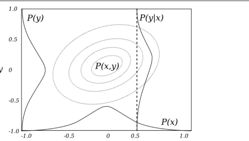
P(x,y) P(y) P(x) -1.0 y 0 0.5 1.0 -1.0 -0.5 -0.5 0 0.5 1.0 P(y|x)

Figure 1.7: Illustration of the Bayes’ theorem for the two-dimensional case. Adapted from

Rodgers(2000).

1.1.2 Bayesian approach to the inverse problem

The Bayes’ theorem provides the formalism usually adopted to solve for the inverse prob-lem. Its application will be illustrated first in the case of scalars, and then generalized to the vector case. In Figure1.1a point in flux space xbbearing an uncertainty σbis equivalent to

formulate that there is a probability density function (PDF) with mean xband standard

de-viation σb. The same statement applies to an observation with errors. This way, the model

projects the prior flux PDF into the observation space. After inversion, the optimized flux can be also described by a PDF with mean xa and uncertainty σa. Its projection into the

observation space would lie in the intersection of the PDFs of the prior and the observa-tion. The interest lies in describing the intersection of those PDFs. Figure1.7illustrates a two-dimensional space defined by scalars x and y. P(x) represents the probability of x being in (x + dx). Similarly, P(y) represents the probability that y lies in (y + dy). Contours represent P(x,y), the joint probability of x being in (x + dx) and y being in (y + dy). If one had some prior estimate of x then one could define P(y|x) as the probability of y being in (y + dy)for a given value x.

From Figure1.7 we can see that P(x) can be obtained by integrating P(x,y) along all the values of y

P(x) = Z ∞

−∞P(x, y)dy (1.2)

P(y)an be calculated by integrating P(x,y) along all the values of x. P(y|x) is propor-tional to P(x,y) as a function of y. SinceR

P(y_{|x) = 1, then it follows}

P(x_{|y) =}R P(x, y)

P(x, y)dy (1.3)

Substituting in the previous equation, we can formulate P(x) as

P(x) = P(x, y)

P(y|x) (1.4)

(20)

P(y) = P(x, y)

P(x_|y) (1.5)

Combining both equations, we obtain

P(x|y) =P(y|x)P(x)

P(y) (1.6)

Equation (1.6) is the Bayes’ theorem. The left-hand term is the posterior PDF of x, which denotes the updated prior estimate of x based on the information contained in the observation. P(y) is independent of x and is usually taken as a normalizing factor.

Assuming Gaussian, unbiased distributions of the errors in x and y (Tarantola,2005), one can write:

P(x) = 1 σb √ 2πexp[− (x_{− x}b)2 2σ2 b ] (1.7)

where xb is the prior estimate of x with an error σb. In the case of the observation,

recalling the link between the fluxes and the observations, provided by the model H, we have P(y_{|x) =} 1 σo √ 2πexp[− (y− H(x))2 2σ2 o ] (1.8)

where σois the observation error. Substituting these two equations in the Bayes’

theo-rem and ignoring the normalizing factor one obtains:

P(x|y) ∼ exp[−(x− xb) 2 2σ2 b −(y− H(x)) 2 2σ2 o ] (1.9)

In the Bayesian framework, the optimal solution for x is the one that maximizes the posterior PDF. The optimal value xa can be obtained by finding the minimum of the cost

function J(x) = (x− xb) 2 σ_b2 + (y_{− H(x))}2 σo2 (1.10) Generalizing this to the vector case, we obtain

J(x) = 1

2(x− xb)TB−1(x− xb) +1

2(yo− H(x))TR−1(yo− H(x)) (1.11)

where xb is the control vector gathering the parameters (i.e. fluxes) controlled by the

inversion and yorepresents the set of observations, respectively. The errors in xband yoare

organized in matrices, and since they may be correlated, B and R are called the variance-covariance matrices of the errors in the prior and in the observations, respectively.

Assuming the transport model is linear (see next Section), i.e., it can be represented as a matrix, Equation1.11can be written as

J(x) = 1

2(x− xb)TB−1(x− xb) +1

2(yo− Hx)TR−1(yo− Hx) (1.12)

The set of optimal fluxes xais the one for which the gradient of J(x) equals zero, and is

(21)

xa= xb+ BHT(HBHT+ R)−1(yo− Hxb) (1.13)

This equation can be written as

xa= xb+ K(yo− Hxb) (1.14)

where K is called the gain, or weight, matrix

K = BHT(HBHT+ R)−1 (1.15)

or alternative as (Bouttier and Courtier,2002)

K = (B−1+ HTR−1H)−1HTR−1 (1.16)

As explained in the next section, how the gain matrix is formulated has an important implication on the numerical solution of the inverse problem.

Note that (1.13) gives the statistically optimal fluxes we look for. But the complete solution to the inverse problem is a PDF, also Gaussian and unbiased, with expected value xaand covariance matrix A given by

A = (I− KH)B (1.17)

Or alternatively,

A = (B−1+ HTR−1H)−1 (1.18)

As with the gain matrix, the choice between (1.17) or (1.18) will depend on the di-mensions of the inversion problem (see next section).

1.1.3 Solution of the inverse problem

Analytical method

In the analytical method, the control vector does not involve directly the fluxes. Instead the elements of x are scaling factors that are applied to the fluxes. Thus each scaling factor corresponds to the flux budget for a given geographic area, period and flux type. The flux budgets are contained in the matrix H.

Han be seen as the combination of three operators (Wu et al.,2016):

H = HsampleHtranHdist (1.19)

The first operator, Hdist, maps each scaling factor in x to CO2fluxes on the grid of the

transport model. These fluxes are known as a basis function. The second operator, Htran,

is an atmospheric transport model that maps the base functions to concentrations of CO2.

Finally, Hsample generates the elements of H by sampling the output the transport model

at the location and time of the observations in yo. The elements of H are referred to as

response functions. Note that there might be parameters not controlled by the inversion. Their response function is included in a vector yfix, and (1.14) can be written as

(22)

1.2. Estimates of CO2 fluxes in Amazonia from atmospheric inversion

The analytical method allows obtaining the explicit values of xa and its uncertainties.

The feasibility of the method depends on the size of the problem. Calculating the matrix Himplies a transport simulation for each base function. In (1.15) and (1.16), calculating the gain matrix implies the multiplication of matrices with dimensions of the control and observation vectors. Therefore, the approach is impractical when both the number of control parameters and the number of observations is very large.

Solving for xa depends on the formulation of K according to (1.15) or (1.16). The

choice depends on the number n of parameters in the control vector and the number of observations m. If (1.15) is chosen, the operation implies calculating a matrix of m × m elements. This is feasible if the number of observations is small. On the other hand, with (1.16), calculating K, a matrix of size n × n, is viable if the number of control parameters is small. For very large problems, the variational approach is more convenient.

Variational method

Instead of calculating the gain matrix explicitly, the variational approach solves for the optimization problem by searching for an approximate optimal solution in an iterative manner (Bouttier and Courtier,2002). The method approaches the minimum of the cost function J(x) using a descent algorithm, evaluating iteratively the cost function and its gradient

∇J(x) = B−1(x− xb) + HTR−1(yo− H(x)) (1.21)

This assumes the forward model H is linear. However, the discretization of the transport equations introduces some non-linearities. The approach is to linearize H about a point x0 so that H(x) − H(x0)≈ H(x − x0). H is called the tangent linear of H about x0. The

minimization process stops either when a limiting number of iterations has been achieved, or when the norm of the gradient reaches a predefined threshold.

1.2 Estimates of CO

₂

fluxes in Amazonia from atmospheric

inversion

Data paucity is limitation of global inversion systems to infer surface fluxes. Most sampling sites across the globe have been chosen to detect large-scale signals and avoid the influ-ence of local fluxes; remote locations on land and ocean have been usually preferred for this purpose, leaving continental areas, like Amazonia, mostly undersampled. The most recent inversion intercomparison study from (Peylin et al.,2013) gathered results from 11 global inversion systems assessed in the frame of the RECCAP initiative (Reginal Carbon Cycle Assessment and Process;Canadell et al.,2011). With different monitoring network configurations among them, none of the systems assimilated observations within tropical South America, much less in Amazonia, as shown in Figure1.8.

Typically, global inversion results vary widely across Amazonia. Differences in trans-port models, prior fluxes, spatial and temporal discretization of the control parameters, observation network configuration and the inversion algorithm, to name a few key system attributes, contribute to the spread among their results, basically because there are no data within the Amazon basin.

Figure1.9shows the spatial distribution of mean annual land CO2fluxes (i.e., excluding

(23)

-50 0 50 -150 -100 -50 0 50 100 150 Longitude La tit ud e 1 2 3 4 5 7 9 10 11

Figure 1.8: Map of site locations used by any of the inversions assessed byPeylin et al.

(2013). Colors represent the number of inversion systems that use that site. Adapted from

Peylin et al.(2013).

et al.(2013). The posterior flux patterns illustrate that in some inversions Amazon fluxes

were optimized using a few scaling factors (e.g. Figure1.9a), or even a single adjustment factor (e.g. Figure1.9h). Other inversions used regular horizontal grid-cells (e.g. Figure

1.9e), with several cells within the Amazon basin, which provides more information about the potential heterogeneity of Amazon fluxes than inversions where Amazon fluxes were controlled using one single scaling factor.

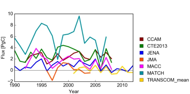
Differences in inversion fluxes are reflected in the inter-annual variations as well. Fig-ure 1.10 illustrates the time series of annual natural flux (excluding fire emissions) in tropical South America, a region containing mainly the Amazon basin, using Transcom’s region definition, from the 11 inversion compared inPeylin et al.(2013). In Figure1.10

there exists a large spread among the inversion estimates, and inversions disagree on the magnitude of the flux anomalies during specific extreme climatic events that have affected Amazonia, such as the droughts of 2005 and 2010.

There exists a large spread in the mean seasonal cycle of NEE over the tropical South America region as well. Figure1.11shows the mean monthly NEE averaged over the period 2000 – 2008 for 7 inversions gathered by Peylin et al. (2013). In general, inversions indicate that vegetation have a peak of CO2 uptake after the onset of the dry season in

most of the Amazon basin, between April and May, associated with the end of the South American Monsoon System (SAMS). CO2 uptake decreases during the transition between

dry and wet seasons, between September and October, and the region turns into a source of CO2 during the wet season during November – March.

The lack of observations in the tropical South America region is at the origin of the seasonal and inter-annual differences of the NEE in (mainly) the Amazon region, as given by global inversions. To illustrate this, it is interesting to look at the results from the study ofStephens et al.(2007). They evaluated the fit of 12 inversions systems—used in the Transcom 3 Level 2 inter-comparison experiment—to the mean annual daytime CO2

vertical gradient between 1 and 4 km, averaged over 12 locations. Each inversion system is represented with a different letter in the Figure1.12.

The models’ mean annual land carbon flux over the period 1992 – 1996 is plotted as a function of their predicted CO2 vertical gradient. Stephens et al. (2007) found that

(24)

1.2. Estimates of CO2 fluxes in Amazonia from atmospheric inversion

Figure 1.9: Annual mean natural CO2 flux for tropical South America, as defined in the

Transcom project, for 2000 for 8 inversion models submitted to RECCAP. Source: http:

//transcom.lsce.ipsl.fr.

the models that were consistent with the observed CO2 vertical gradient also estimated

a weaker Northern latitude sink, and a smaller tropical source. Since seasonal actions between atmospheric mixing and NEE in the Northern Hemisphere create inter-hemispheric annual CO2 gradients, and because the global mass balance of atmospheric

(25)

Figure 1.10: Annual natural CO2flux (excluding fire emissions) for tropical South America

(Transcom definition) from 1990 to 2012 for the 7 inversion models submitted to RECCAP. Source:http://www.globalcarbonatlas.org.

Figure 1.11: Mean monthly natural CO2 flux for tropical South America (Transcom

def-inition) from 2000 to 2008 for 7 inversion models submitted to RECCAP. Adapted from

(26)

1.3. Toward robust inverse modeling estimates of CO2fluxes in Amazonia A C 26 B 3 89 1 7 45 r = 0.542 A C 2 6 B 3 89 1 7 45 r = 0.762 6 4 2 0 -2 -4 -6 0.0 0.5 1.0 1.5 2.0 2.5 2 Annual means Post-in ver sion flux [PgC yr -1 ] Observed Δ 1 - C Northern land 1 - C Tropical land 1 km - 4 km CO (ppm)₂

Figure 1.12: Mean annual Northern and tropical land carbon flux averaged over 1992 – 1996, estimated by the 12 inversion systems evaluated in 12 TRANSCOM3 Level 2 exper-iment, as a function of models’ estimated mean vertical CO2 gradient beetween 1 and 4

km. Vertical axis: estimated flux for northern (red) and tropical (blue) land regions. Hor-izontal axis: predicted 1 km - 4 km CO2 gradient. Numbers (1 – 9) and letters (A – C)

represent the models’ estimates. Grey bar: represents the observed gradient (center) and its uncertainty (width). Adapted fromStephens et al.(2007).

tropical land fluxes. Thus, Figure 1.12illustrates that systematic errors in the covariance between seasonal transport and NEE in the Northern Hemisphere induce an overestimation of the northern land sink, compensated by a stronger tropical land source. This means that in a region like Amazonia, with scarce observations of the atmosphere inside and around the region, local fluxes estimated through inversion are subject to misfits in remote sites distant from Amazonia.

In the mid-latitudes, the available potential energy associated with zonal temperature gradients is the main source of energy for synoptic variations. Latent heat and radiative heating play a secondary role in the energetics in these latitudes. In the tropics, however, latitudinal temperature gradients are small and latent heat release, mostly associated with convective cloud systems, appears to be the dominant energy source driving synoptic scale variations (p. 370 – 371;Holton,2004). Thus, while synoptic variations outside the tropics are dominated by horizontal transport, vertical convective mixing prevails in the tropics. Accurate representation of these mechanisms in transport models is crucial in inverse mod-eling systems (Gurney et al.,2003;Parazoo et al.,2008). Errors in the representation of vertical mixing induce biases in their flux estimates (Stephens et al.,2007).

1.3 Toward robust inverse modeling estimates of CO

₂

fluxes in

Amazonia

A few studies have used directly atmospheric CO2 observations to estimate the Amazon

(27)

bal-ance calculations of the atmospheric column to estimate regional CO2 fluxes (Chou et al.,

2002;Lloyd et al.,2007; Wofsy et al.,1988) that are representative of non-characterized

area of central Amazonia. More regular aircraft profiles in the interior of the Amazon, completed by data from coastal sites, have allowed obtaining first estimates of seasonal CO2 budgets for eastern Amazonia (Gatti et al., 2010).With a more complete data set of

biweekly aircraft profiles,Gatti et al.(2014) (GA2014 henceforth) made an unprecedented effort to sample the atmosphere within the Amazon basin in such a way that their obser-vations were sensitive to fluxes over most of the Amazon basin, covering not only a large fraction of Amazon forest areas but capturing the signal of savanna and agricultural lands. GA2014 collected aircraft CO2data over two years with contrasting climatic conditions

in Amazonia. In 2010 the region was anomalously dry for two reasons. During January – March, El Niño caused low precipitation in the northern and central Amazon basin. Then, in the second half of the year a positive anomaly in the North Atlantic sea surface temperature caused the inter-tropical convergence zone (ITCZ) to remain more northerly than usual. This prolonged and intensified the dry conditions in southern parts of the basin. 2011, on the other hand, was an anomalously wet year. With their observations and using a mass balance approach GA2014 calculated basin-wide fluxes over those two years. GA2014 found that during 2010 the Amazon emitted 0.48 ± 0.18 PgC, but was carbon neutral during 2011 (0.06 ± 0.1 PgC yr−1_{). After removing CO}₂_{losses due to fire emissions, they}

found the Amazon basin was nearly neutral (−0.03 ± 0.22 PgC yr−1_{) during 2010, and}

that during the wet year the vegetation was a net sink of 0.25 ± 0.14 PgC yr−1_{, consistent}

with a long-term estimate of 0.39 ± 0.10 PgC yr−1_{from forest censuses. Thus, their results}

highlighted the importance of moisture conditions on the Amazon carbon balance. It was the first that such measurements were used to derive a basin-wide estimate of CO2 fluxes

in Amazonia.

van der Laan-Luijkx et al. (2015) were the first to assimilate the vertical profiles of

GA2014 into a dedicated version of the CarbonTracker global inversion system (Peters

et al., 2007). van der Laan-Luijkx et al. (2015) predicted that during 2010, year of the

drought, the Amazon was net source of 0.07 ± 0.42 to 0.31 ± 0.42 PgC yr−1_{, the range}

being from a set of inversions using different biomass burning estimates. In contrast, dur-ing 2011 the ecosystem turned to net carbon sink of −0.15 ± 0.42 to −0.33 ± 0.46 PgC yr−1_{. These results were consistent with the mass balance approach of GA2014 but}

they gave a slightly smaller difference between 2010 and 2011 than GA2014. Alden et al.

(2016) published results of the assimilation of airborne observations made over the longer period 2010 – 2012 into a regional inversion system, using two transport models. They predicted the Amazon basin to be a source of 0.5 ± 0.3 PgC yr−1 _{during 2010, in}

agree-ment with GA2014, but also estimated a net source of 0.2 ± 0.3 PgC yr−1 _{in 2011 (see}

Figure 3a in Alden et al. (2016)). With a longer observation record by one year, their results showed that during 2012 the vegetation continued to recover from the effects of drought and turned into a large net sink, with a a net uptake larger by 0.68 ± 0.45 PgC yr−1_{in 2010 with respect to 2010.}

In line with the efforts ofvan der Laan-Luijkx et al.(2015) andAlden et al.(2016), the present work in this thesis aim at improving the knowledge of the carbon balance in Ama-zonia using an inverse modeling approach. By the time the present thesis works started in 2012, available data was much more limited with a few ground stations mainly near the coast. Some measurement sites had gaps of several years, and few sites were inter-rupted. With this limited data set, in the chapter On the ability of a global atmospheric inversion to constrain variations of CO2 fluxes over Amazonia (Chapter 2), I analyzed the

(28)

1.4. Structure of this work

seasonal and interannual variations of NEE in Amazonia with two global inversions, as-similating the data from 4 stations around the Amazon in one of them. The study looked at the global inversion results with more detail than previous intercomparison studies and showed the impact of these scarce data on the optimized fluxes. Though, the study re-marked the need for more data, and suggested that assumptions on the prior errors and aspects of representation of the transport in Amazonia should be revisited. In the chap-ter Regional atmospheric modeling of CO2 transport in Amazonia (Chapter 3), I evaluated

the potential improvement brought by a regional atmospheric model, relative to a global one (which assimilates weather data from satellite and stations), when both models were used to force an off-line CTM to simulate CO2 fields in Amazonia. I investigated the

sen-sitivity of the transport of CO2 to different transport components, as a function of four

different observation vectors—based on the vertical profiles of GA2014—to bring insight on the best strategy to assimilate aircraft measurements. Finally, in the chapter Regional atmospheric inversion of CO2in Amazonia(Chapter4), I present the regional inversion

sys-tem I developed, which take advantage of both transport configurations, to optimize NEE using the four observation vectors separately. The chapter brings further information on the consistency and robustness of Amazon NEE from assimilation of different observation types.

1.4 Structure of this work

This dissertation starts with an analysis of the seasonal and interannual variations of the net ecosystem exchange (NEE) in Amazonia over the period 2002 – 2010 (Chapter2). It describes the setup of two global inversion configurations to investigate CO2 fluxes over

the Amazon region, one of which included few ground-based station data that were avail-able before the study of GA2014 and that had not been exploited in previous global inverse modeling studies. As a first indicator of the confidence on the impact of assimilating these new data, the impact on the posterior concentration time series at the new sites (Section

2.2.1) was characterized, followed by the analysis of the impact on the fluxes (Section

2.2.2). The spatial distribution of flux increments by both inversions was analyzed as a measure of the confidence on the improvement of the simulated seasonal cycle and in-terannual variability (Section 2.2.2) of NEE in Amazonia, both at basin and sub-regional scale.

The data collected by GA2014 have filled a major information gap in inverse modeling studies over Amazonia. The combination of new data and modeling tools, motivated the second part of my research (Chapter3), which aimed at evaluating whether CO2transport

in Amazonia could be improved with the meteorology generated with the regional atmo-spheric model BRAMS, developed for simulating meteorology and chemistry over tropical South America, with respect the global forecast system ECMWF. Thus, two transport con-figurations were setup (Section 3.1.1). The meteorology of both models was evaluated against ground-based, remote-sensing and satellite observations (Section3.2.1). The qual-ity of the simulated CO2 fields by both models is assessed (Section 3.2.2). With the data

of GA2014, not only vertical profiles were evaluated. These data allowed evaluated the quality of the horizontal transport. This chapter gives an estimate of the uncertainty of CO2 related to differences between the two transport models, which are prescribed with

the same surface fluxes.

(29)

in-version systems (Section4.1) based on the forward transport configurations evaluated in Chapter3. Individual inversions were performed with different observation vectors, in-cluding vertical profiles and different types of horizontal gradients, with both inversion systems. The study evaluated the fit to the observations (Section4.2), and the impact on the optimized fluxes (Section 4.3). Finally, Chapter 5 presents a summary of the main results this thesis, as well as suggestions on the orientation of future research.

(30)

CHAPTER

2 On the ability of a global

atmospheric inversion to

constrain variations of CO

₂

fluxes over Amazonia

When starting the thesis in 2012, there existed few sampling sites in South America with CO2 measurements with sufficient precision to be used in atmospheric inversion studies.

However, these data had not been assimilated in most global inversion systems (Peylin

et al.,2013). Motivated by this, I assimilated CO2data from some of the few ground-based

stations were available at the time into a global inversion system, aiming at improving the knowledge on the seasonal and interannual variations of the net ecosystem exchange in Amazonia, and assess the impact of local observation sites in the global system. The results of this chapter lead to the publication "On the ability of a global atmospheric inversion to constrain variations of CO2 fluxes over Amazonia" in the journal Atmospheric Chemistry

and Physics (Molina et al.,2015). The study is presented in Section 2.1, the main results and their implications are detailed in Section 2.2, and the concluding remars in Section

2.3. The whole publication is given in the AppendixA.

2.1 Objective of the study

The study aimed at improving our knowledge of the seasonality and interannual variations of NEE in Amazonia over the period 2002 – 2010. This period is long enough to assess the impact of extreme climatic events such as the severe droughts of 2005 and 2010, and the extreme humid conditions registered in 2009. For this purpose, I designed an inversion, referred to as INVSAm henceforth, by building on the Monitoring of Atmospheric Climate and Compositon (MACC) global inversion system version 10.1 (MACCv10.1 hereafter), described in detail by (Chevallier et al.,2010). Both INVSAm and MACCv10.1 optimized a prior NEE estimate simulated with the ecosystem model ORCHIDEE by Maignan et al.

(2011). Ocean fluxes were also optimized, but the study focused on the corrections to the NEE.

MACCv10.1 assimilated data from about 100 sampling sites around the globe, but none were located in Amazonia. To improve the NEE estimate, INVSAm added four local sites. Two sampling sites were located at Arembepe and Maxaranguape, on the eastern coast of Brazil, basically under marine influence, measured the background CO2. The other

(31)

tropical forests and captured the signal of terrestrial ecosystems. This way, the impact of local data on the optimized fluxes was assessed against MACCv10.1. In addition, the study went deeper than previous inversion intercomparison studies such as TRANSCOM and RECCAP (Canadell et al., 2011), since it evaluated the inversion results over and within Amazonia in an attempt to identify robust patterns.

2.2 Main results and implications

2.2.1 Simulated vs. observed concentrations

Overall, both INVSAm and MACCv10.1 significantly reduced the misfit to the observations with respect to the prior. However, misfits were further decreased with the assimilation of data in South America. Examination of simulated CO2time series at the local sites, showed

that assimilating local data significantly rescaled the seasonal variations (e.g. at the site in French Guiana), and even changed the seasonality (e.g. at Santarém and Maxaranguape) in agreement with the observations, with respect to the reference inversion. Correlation be-tween time series of optimized and observed daily concentrations were rather low in both inversions at the four local sites. However, correlations at monthly scale were higher with both inversion estimates, and again, INVSAm showed better correlation than MACCv10.1. This suggested a potential improvement of seasonal variations of NEE in Amazonia.

2.2.2 Impact on surface biogenic CO2 fluxes

Spatial distribution of flux corrections

In terms of the spatial distribution of flux corrections, both INVSAm and MACCv10.1 pre-dicted large continuous, nearly zonal patterns that extended over both land and ocean, likely due to the dominant atmospheric circulation. On the continent, both inversions pre-dicted flux corrections of opposite sign between north and south of tropical South America, between austral summer and winter and at the annual scale. This result is typical of inver-sion systems over undersampled regions. The assimilation of the local stations, however, did increase the amplitude of the dipole. Flux corrections by INVSAm often exceeded 150% of the prior fluxes (in absolute value), indicative of significant flux corrections. In addi-tion, with local data the inversion changed the latitudinal position of the dipole over the continent. This provides evidence of the large-extent impact of the information from local stations, despite the relatively small correlation scale length in prior uncertainties, and the limited area of the station footprints with high sensitivity to land fluxes.

Seasonality

At the scale of tropical South America, the seasonal cycle of optimized NEE in both IN-VSAm and MACCv10.1 seemed strongly driven by the prior NEE. Nevertheless, while flux corrections introduced by local data likely came from the signal of tropical broad-leaved (TBE) forests, the seasonal cycle could have remained driven by the NEE from other plant functional types (PFTs) represented in ORCHIDEE. Over TBE forests, however, prior and inversion estimates did not indicate clear correlation of NEE with rainfall or solar radia-tion. The results disagreed with the estimate ofJung et al.(2011). Prior and inverted NEE indicated local extremes, possible due to the overlapping of significantly different seasonal cycles from other subregions within Amazonia.

(32)

2.2. Main results and implications

To examine if the inversions captured the potential spatial heterogeneity of NEE sea-sonality, two sub-regions were analyzed. Nevertheless, neither the prior nor the inversions indicated a clear seasonal cycle. Jung et al.(2011), on the other hand, continued to ex-hibit a smooth seasonal cycle, of nearly the same amplitude in both sub-regions and across all TBE forests. This reduced the confidence in Jung et al. (2011) to capture the spatial heterogeneity seasonal NEE variations. Within the two sub-regions, results suggested sig-nificant corrections to the seasonal cycle of NEE, especially over regions well constrained, in space and time, by the observation sites. However, large corrections were also applied over areas over which the local stations exhibited low sensitivity, particularly in central western Amazonia. This can be partly explained by the control exerted on the optimized fluxes by the local stations, as well as stations distant from Amazonia, suggested by the analysis of the spatial distribution of flux corrections. This is a direct consequence of the limited overlapping between measurement records at the local sites.

Inter-annual variations

The analysis of the inversions’ ability to capture the interannual variability of NEE within Amazonia focused on the drought periods recorded in 2005 and 2010, and the extreme hu-mid conditions of 2009. The analysis was based on NEE anomalies with respect the mean NEE during 2002 – 2010 predicted by the different estimates. Thus, from the atmospheric perspective, negative anomalies were interpreted as an enhancement of the CO2sink, and

positive anomalies as a reduction. I made an additional inversion using a "flat prior" (called FLAT), i.e., prior NEE without interannual variability with respect to the mean NEE 2002 – 2010 across tropical South America (see the publication in AppendixAfor details). The goal was to assess the inversion system’s ability to reproduce interannual variations from the observations alone, a potential indicator of the robustness of the inversion estimates.

Literature reports on the intensity and extension of the drought events of 2005 and 2010, and their negative effects on Amazonian forests. Nevertheless, across tropical South America prior NEE and both INVSAm and MACCv10.1 estimates indicated only small pos-itive anomalies in those years, while FLAT predicted pospos-itive and negative anomalies in 2005 and 2010, respectively. In 2009, on the other hand, prior and inversion estimates all agreed on a large negative anomaly, which provided confidence on this pattern. Over TBE forests, prior and both INVSAm and MACCv10.1 predicted a positive anomaly in 2005 and negative in 2010. The latter contrasts not only with the anomalies inferred for the whole tropical South America, but also with the findings of Gatti et al.(2014). Their re-sults, obtained using a mass balance approach and airborne CO2 and CO observations,

indicated CO2 uptake reduction due to water stress during 2010 across Amazon forests.

My results, therefore, are to be interpreted cautiously, as the small anomalies, compared to those considering all PFTs, suggest low NEE sensitivity in TBE forests to interannual climatic variations.

Interannual variations within the subregions examined in the analysis of seasonal vari-ability revealed contrasting responses to drought events within and between the regions. While in eastern Amazonia the prior and both INVSAm and MACCv10.1 predicted posi-tive and negaposi-tive anomalies in 2005 and 2010, respecposi-tively, in central western Amazonia anomalies were negative in both years. Anomalies in J2011 were at least one order of magnitude smaller than the prior and both inversion estimates. Consequently, J2011 did not provide enough information on the heterogeneity of NEE interannual variations and help interpret my results.

(33)

2.3 Conclusions

In an effort to improve the knowledge on the seasonal and interannual variations of NEE in Amazonia I analyzed the results two global inversions, and assimilated data from four ground-level sites in tropical South America in one of the inversions. The results showed that information from both local and distant sampling sites controlled NEE in tropical South America. This control manifested as alternate zonal areas of positive and negative flux corrections over land and over large portion of the ocean in the Southern Hemisphere in a "dipole" pattern. The main effect of the local ground-based station data was to increase the amplitude of the dipole and change its position, and create some local patterns around the local sites.

In spite of the overall improvement of seasonal variations of the simulated CO2

concen-trations at the local sites, the seasonal cycle of NEE over tropical South America remained mostly unchanged in the inversion estimates. Particularly over rain forests, prior and in-version estimates disagreed with the assumption of higher CO2 uptake during periods of

higher solar radiation. The smooth patterns of NEE inJung et al. (2011) disagreed with my results. The low reliability on the seasonal patterns of NEE from the inversions seems to confirm that the spatial distribution of flux corrections over the entire Amazon basin is an artifact from the inversion, reflecting the low density of the local monitoring network, and the limited measurement records.

Such considerations also reduce the confidence on the patterns of NEE interannual variability from the inversion INVSAm. Yet, some patterns were present across prior and inversion estimates, suggesting they are robust, such as the vegetation being a net source of CO2(∼ 0.21 PgC) during 2005—year of the drought—and a strong sink (∼ −1.1 PgC)

(34)

CHAPTER

3 Regional atmospheric modeling

of CO

₂

transport in Amazonia

The analysis in Chapter2reveals the limitations of the global-scale atmospheric inversion approach to estimate the CO2net ecosystem exchange (NEE) over the Amazon basin, even

when assimilating regional CO2 observations. In particular, it highlights the difficulties

to simulate the concentrations at the measurement sites, especially near the coast, with a coarse resolution global-scale transport model like LMDZ. The representativeness and transport modeling errors of this global model are assumed to be two of the main expla-nations for the lack of ability to control the regional NEE in the inversion experiments presented in Chapter2. In order to overcome such issues, I have developed regional and mesoscale atmospheric transport model configurations for the Amazon basin. This chapter presents these configurations and the evaluation of their skill for modeling the regional CO2transport while Chapter4will analyze the regional atmospheric inversions that I have

conducted with these transport configurations.

When using regional transport model instead of global models, the simulations of the CO2 transport can be improved both by increasing the spatial resolution and by using

the meteorological forcing from regional meteorological models that are adapted to the specific conditions in the area of interest. The Brazilian developments on the Regional Atmospheric Modeling System (BRAMS; Freitas et al., 2009; Moreira et al., 2013) has been specifically developed to better represent meteorology and atmospheric chemistry-transport over South America. In Amazonia, vertical chemistry-transport due to moist convection is a dominant process over advection, and largely explains synoptic variations of atmospheric

CO2 (Parazoo et al., 2008). BRAMS includes new physical schemes to better represent

deep and shallow convection in the Amazon (Freitas et al., 2009). Another important source of uncertainty in model simulations is the strong dependency on the representation of surface processes. In this regard, BRAMS has been coupled "on-line" with the JULES land surface scheme, which has improved the representation of several meteorological variables

(Moreira et al.,2013).

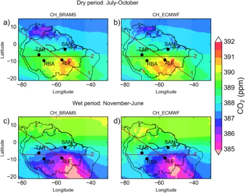
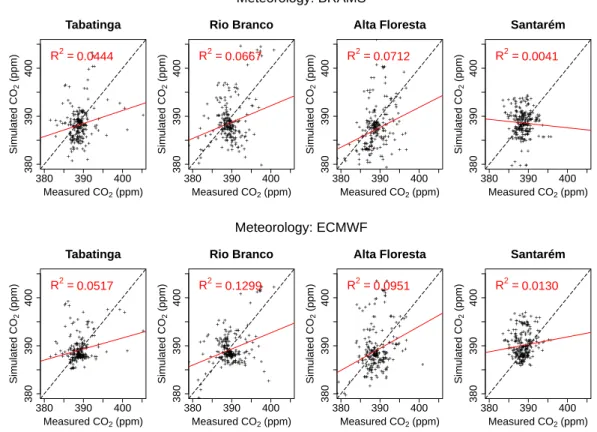
I prepared two regional transport configurations to simulate CO2 transport over

tropi-cal South America at a high resolution of ∼ 35 km for the year 2010. I used the mesostropi-cale and regional tracer-transport model (CTM) CHIMERE (Menut et al., 2013), driven with different meteorological fields provided by two atmospheric models: the integrated fore-cast system of the European Centre for Medium-Range Weather Forefore-casts (ECMWF), and

Modélisation inverse des flux de CO2 en Amazonie

HAL Id: tel-01697602

https://tel.archives-ouvertes.fr/tel-01697602

To cite this version:

M

ODÉLISATION

I

NVERSE DES

F

LUX DE

CO

EN

A

MAZONIE

Thèse de doctorat

de l’Université Paris-Saclay

préparée à l’Université de Versailles Saint-Quentin-en-Yvelines

Ecole doctorale N

129

Sciences de l’Environnment en Ile-de-France (SEIF)

Spécialité de doctorat: Météorologie, océanographie et physique de

l’environnement

Thèse présenté et soutenue à Gif sur Yvette, le 24 octobre 2017, par

M. L

UIS

MOLINA CARPIO

Contents

1

CO

2

exchanges by land

ecosystem in Amazonia inferred

from atmospheric inversion

1.1 Principles of the inverse problem

a)

b)

1.2 Estimates of CO

fluxes in Amazonia from atmospheric

inversion

1.3 Toward robust inverse modeling estimates of CO

fluxes in

Amazonia

1.4 Structure of this work

2

On the ability of a global

atmospheric inversion to

constrain variations of CO

2

fluxes over Amazonia

2.1 Objective of the study

2.2 Main results and implications

2.3 Conclusions

3

Regional atmospheric modeling

of CO

2

transport in Amazonia

₁₂₉

₂

₂

₂