HAL Id: tel-02125289
https://tel.archives-ouvertes.fr/tel-02125289
Submitted on 10 May 2019
HAL is a multi-disciplinary open access archive for the deposit and dissemination of sci-entific research documents, whether they are pub-lished or not. The documents may come from teaching and research institutions in France or abroad, or from public or private research centers.
L’archive ouverte pluridisciplinaire HAL, est destinée au dépôt et à la diffusion de documents scientifiques de niveau recherche, publiés ou non, émanant des établissements d’enseignement et de recherche français ou étrangers, des laboratoires publics ou privés.
Etude du cycle biogéochimique du fer : distribution et
spéciation dans l’Océan Atlantique Nord (GA01) et
l’Océan Austral (GIpr05) (GEOTRACES)
Manon Tonnard
To cite this version:
Manon Tonnard. Etude du cycle biogéochimique du fer : distribution et spéciation dans l’Océan At-lantique Nord (GA01) et l’Océan Austral (GIpr05) (GEOTRACES). Geochemistry. Université de Bre-tagne occidentale - Brest; Université de Tasmanie (Australie), 2018. English. �NNT : 2018BRES0115�. �tel-02125289�
THESE DE DOCTORAT EN CO-TUTELLE INTERNATIONALE DE
L'UNIVERSITEDEBRETAGNEOCCIDENTALE
COMUE UNIVERSITE BRETAGNE LOIRE
ECOLE DOCTORALE N°598
Sciences de la Mer et du littoral
Spécialité : Chimie marine
AVEC L’UNIVERSITEDETASMANIE
I
NSTITUT D’E
TUDESM
ARINES ETA
NTARCTIQUES Spécialité : Sciences Marines et AntarctiquesPar
Manon TONNARD
Etude du Cycle Biogéochimique du Fer : Distribution et spéciation dans
l’Océan Atlantique Nord (GA01) et l’Océan Austral (GIpr05) (GEOTRACES)
Thèse présentée et soutenue à l’Institut Universitaire Européen de la Mer, Technopôle Brest-Iroise, Rue Dumont d’Urville, 29280 Plouzané, le 6 Juillet 2018
Unité de recherche : Laboratoire des sciences de l’Environnement MARin - UMR 6539 (LEMAR) et Centre de Recherche Coopérative sur le Climat et les Ecosystèmes Antarctiques
Rapporteurs avant soutenance :
Cécile GUIEU
Directrice de Recherche CNRS, Laboratoire d'Océanographie de Villefranche-sur-Mer (LOV), UMR 7093, CNRS, Université Pierre et Marie Curie, Observatoire Océanologique de Villefranche-sur-Mer
Christoph VÔLKER
Docteur, Alfred-Wegener-Institut Helmholtz-Zentrum für Polar-und Meeresforschung, Germany
Composition du Jury :
François LACAN
Directeur de Recherche CNRS, Laboratoire d'Etudes en Géophysique et Océanographie Spatiales (LEGOS), UMR 5566, CNRS/IRD/CNES/UPS, Université de Toulouse, Observatoire Midi-Pyrénées Président du Jury
Cécile GUIEU
Directrice de Recherche CNRS, Laboratoire d'Océanographie de Villefranche-sur-Mer (LOV), UMR 7093, CNRS, Université Pierre et Marie Curie, Observatoire Océanologique de Villefranche-sur-Mer
Christoph VÖLKER
Docteur, Alfred-Wegener-Institut Helmholtz-Zentrum für Polar-und Meeresforschung, Germany
Julia UITZ
Docteur, Laboratoire d'Océanographie de Villefranche-sur-Mer (LOV), UMR 7093, CNRS, Université Pierre et Marie Curie, Observatoire Océanologique de Villefranche
Simon USSHER
Professeur agrégé de Chimie Marine et Analytique, School of Geography, Earth and Environmental Sciences, University of Plymouth, England
Géraldine SARTHOU
HDR, Directrice de Recherche CNRS, Laboratoire des Sciences de l’Environnement MARin (LEMAR), UMR 6539, CNRS/IUEM/IRD/Ifremer, Université de Bretagne Loire, Brest, Directrice de thèse
Andrew R. BOWIE
Professeur agrégé, Antarctic Climate & Ecosystems Cooperative Research Centre (ACE-CRC), Institute for Marine and Antarctic Studies (IMAS), University of Tasmania, Hobart AUS (TAS), Directeur de thèse
Hélène PLANQUETTE
Statements and declarations
Declaration of Originality
This thesis contains no material which has been accepted for a degree or diploma by the University or any other institution, except by way of background information and duly acknowledged in the thesis, and to the best of my knowledge and belief no material previously published or written by another person except where due acknowledgement is made in the text of the thesis, nor does the thesis contain any material that infringes copyright.
Authority of Access
This thesis may be made available for loan and limited copying and communication in accordance with the Copyright Act 1968.
Statement regarding published work contained in the thesis
The publishers of the papers comprising Chapters 3 to 5 hold the copyright for that content, and access to the material should be sought from the respective journals. The remaining non published content of the thesis may be made available for loan and limited copying and communication in accordance with the Copyright Act 1968.
Statement of co-authorship
The following people and institutions contributed to the publication of work undertaken as part of this thesis:
Candidate Manon Tonnard ACE-CRC/IMAS - University of Tasmania
LEMAR/IUEM, CNRS UMR 6539 - Université de Bretagne Loire
Author 1 Géraldine Sarthou, Supervisor LEMAR/IUEM, CNRS UMR 6539 - Université de Bretagne Loire
Author 2 Andrew R. Bowie, Supervisor ACE-CRC/IMAS - University of Tasmania
Author 3 Hélène Planquette, Co-Supervisor LEMAR/IUEM, CNRS UMR 6539 - Université de Bretagne Loire
Author 4 Pier van der Merwe, Co-Supervisor ACE-CRC - University of Tasmania
Author 5 Morgane Gallinari LEMAR/IUEM, CNRS UMR 6539 - Université de Bretagne Loire
Author 6 Florianne Desprez de Gésincourt LEMAR/IUEM, CNRS UMR 6539 - Université de Bretagne Loire
Author 7 Yoan Germain Laboratoire Cycles Géochimiques et ressources, Ifremer
Author 8 Arthur Gourain Ocean Sciences Department, School of Environmental Sciences - University of Liverpool
Author 9 Marion Benetti Institute of Earth Sciences - University of Iceland
LOCEAN, CNRS UMR 7159, IRD, MNHN - Sorbonne Universités
Author 10 Gilles Reverdin LOCEAN, CNRS UMR 7159, IRD, MNHN - Sorbonne Universités
Author 11 Paul Tréguer LEMAR/IUEM, CNRS UMR 6539 - Université de Bretagne Loire
Author 12 Julia Boutorh LEMAR/IUEM, CNRS UMR 6539 - Université de Bretagne Loire
Author 13 Marie Cheize LEMAR/IUEM, CNRS UMR 6539 - Université de Bretagne Loire Laboratoire des cycles Géochimiques –Centre Ifremer Bretagne
Author 14 Jan-Lukas Menzel Barraqueta GEOMAR Helmholtz-Zentrum für Ozeanforschung
Author 15 Leonardo Pereira Contreira Fundação Universidade Federal do Rio Grande (FURG)
Author 16 Rachel Shelley Dept. Earth, Ocean and Atmospheric Science - Florida State University School of Geography, Earth and Environmental Sciences - University of Plymouth
LEMAR/IUEM, CNRS UMR 6539 - Université de Bretagne Loire
Author 17 Pascale Lherminier Laboratoire d'Océanographie Physique et Spatiale (LOPS)/IUEM/ Ifremer/CNRS/IRD - Université de Bretagne Loire
Author 18 Anne Donval LEMAR/IUEM, CNRS UMR 6539 - Université de Bretagne Loire
Author 19 Luis Lampert Laboratoire d’Ecologie Pélagique – Ifremer
Author 20 Hervé Claustre Laboratoire d'Océanographie de Villefranche-sur-Mer (LOV), CNRS UMR 7093 - Université Pierre et Marie Curie
Author 21 Celine Dimier Laboratoire d'Océanographie de Villefranche-sur-Mer (LOV), CNRS UMR 7093 - Université Pierre et Marie Curie
Author 22 Joséphine Ras Laboratoire d'Océanographie de Villefranche-sur-Mer (LOV), CNRS UMR 7093 - Université Pierre et Marie Curie
Author 23 Raphaëlle Sauzède Laboratoire d'Océanographie de Villefranche-sur-Mer (LOV), CNRS UMR 7093 - Université Pierre et Marie Curie
Author 24 Lorna Foliot Laboratoire des Sciences du Climat et de l'Environnement, Gyf-sur-Yvette, France
Author 25 Kathrin Wuttig ACE-CRC - University of Tasmania
Author 26 Thomas Holmes ACE-CRC/IMAS - University of Tasmania
Author 27 Ashley Townsend Central Science Laboratory - University of Tasmania
Author 28 Zanna Chase IMAS - University of Tasmania
Author 29 Lavenia Ratnarajah Ocean Sciences Department, School of Environmental Sciences - University of Liverpool
Author details and their roles:
Paper 1 – Tonnard, M., Planquette, H., Bowie, A. R., van der Merwe, P., Gallinari, M., Desprez de Gésincourt, F., Germain, Y., Gourain, A., Benetti, M., Reverdin, G., Tréguer, P., Boutorh, J., Cheize, M., Menzel Barraqueta, J. L., Pereira-Contreira, L., Shelley, R., Lherminier, P. and Sarthou, G. Dissolved iron in the North Atlantic Ocean and Labrador sea along the GEOVIDE section (GEOTRACES section GA01) (submitted to Biogeosciences), Located in Chapter 3
Candidate contributed to the statistical analysis of the data set and the writing up of the manuscript. Authors 1, 2, 3 and 4 contributed to the preparation of manuscript and authors 1 and 3 also contributed to DFe sample collection. Authors 5, 6 and 7 contributed to the DFe analysis on the seaFAST-picoTM SF-ICP-MS. Author 8 contributed to the analysis of Particulate Fe data and their interpretation. Authors 9 and 10 contributed to the estimation of the sea-ice melting, sea-ice formation and meteoric water fractions and their interpretation. Author 11 and 5 contributed to the analysis of the major nutrients. Authors 12, 13, 14, 15, 16 contributed to DFe sample collection, in addition author 16 contributed to the analysis of the aerosols and their interpretation. Author 17 contributed to the interpretation of water mass circulation and physical processes. Author 1 and 17 were PIs of the GEOVIDE voyage.
Paper 2 – Tonnard, M., Donval, A., Lampert, L., Tréguer, P., Bowie, A. R., van der Merwe, P., Planquette, H., Claustre, H., Dimier, C., Ras, J. and Sarthou, G., Phytoplankton assemblages in the North Atlantic Ocean and in the Labrador Sea along the GEOVIDE section (GEOTRACES section GA01) determined by CHEMTAX analysis from HPLC pigment data: from an assessment of the community structure, succession and potential limitation to broader implication (in prep.),
Located in Chapter 4
Candidate contributed to the statistical analysis of the DFe data set and the writing up of the manuscript. Authors 1, 2, 3 and 4 contributed to the preparation of manuscript and authors 1 and 3 also contributed to DFe sample collection. Author 11 and 5 contributed to the analysis of the major nutrients. Authors 18 and 19 contributed to the building of the initial pigment matrix used in the CHEMTAX model. Authors 23, 24 collected the pigment samples, while authors 20, 21, 22 and 23 contributed to their analysis by HPLC.
Paper 3 – Tonnard, M., Wuttig, K., Holmes, T., van der Merwe, P., Townsend, A., Sarthou, G., Planquette, H., Chase, Z., Ratnarajah, L. and Bowie, A. R., Dissolved and soluble Fe-binding organic ligands near the Kerguelen Archipelago (B-transect) and in the vicinity of Heard and McDonald Islands (HEOBI voyage – GIpr05) (in prep.),
Located in Chapter 5
Candidate contributed to the soluble Fe (SFe), soluble Fe-binding organic ligand (SLt), DFe and dissolved Fe-binding organic ligand (DLt) sample collection, the analysis of SFe on the seaFAST-picoTM and SLt and DLt on a voltammeter, statistical analysis of the data set, and the writing up of the manuscript. Authors 1, 2, 3, 4, 25 contributed to the preparation of manuscript Authors 2, 4, 25, 26, 28 and 29 contributed to DFe, SFe, DLt and SLt sample collection. In addition, authors 4 and 25 contributed to the analysis of SFe, SLt, DFe and DLt and author 26 to the analysis of DFe. Author 27 contributed to the analysis of the DFe and SFe on the SF-ICP-MS.
We the undersigned agree with the above stated “proportion of work undertaken” for each of the above published (or submitted) peer-reviewed manuscripts contributing to this thesis:
Signed Candidate Manon Tonnard
Author 1 Géraldine Sarthou
Author 2 Andrew R. Bowie
Author 3 Hélène Planquette
Author 4 Pier van der Merwe
Author 5 Morgane Gallinari
Author 6 Florianne Desprez de Gésincourt
Author 7 Yoan Germain
Author 8 Arthur Gourain
Author 9 Marion Benetti
Author 10 Gilles Reverdin
Author 11 Paul Tréguer
Author 12 Julia Boutorh
Author 13 Marie Cheize
Author 14 Jan-Lukas Menzel Barraqueta
Author 16 Rachel Shelley
Author 17 Pascale Lherminier
Author 18 Anne Donval
Author 19 Luis Lampert
Author 20 Hervé Claustre
Author 21 Cecile Dimier
Author 22 Joséphine Ras
Auhtor 23 Raphaëlle Sauzède
Author 24 Lorna Foliot
Author 25 Kathrin Wuttig
Author 26 Thomas Holmes
Author 27 Ashley Townsend
Author 28 Zanna Chase
Supervisor and Head of School Declaration
I the undersigned agree with the above stated “proportion of work undertaken” for each of the above published (or submitted) peer-reviewed manuscripts contributing to this thesis.
Signed
Head of School
Institute for Marine and Antarctic Studies University of Tasmania
Acknowledgements
I first want to express my sincere acknowledgements to the jury members who agreed on evaluating my work: thank you very much Cécile Guieu and Christoph Völker for reviewing the thesis, thanks to Simon Ussher, Julia Uitz and François Lacan for examining my work. I would also like to acknowledge Catherine Jeandel and Alessandro Tagliabue who followed my work during my thesis comity and who gave me advices of great value, that allow me to explore new directions.
Throughout these three years and a half (a bit more), I have had the chance to join two diverse and very interesting groups of individuals with years of experience and good advices: thank you so much Géraldine, Hélène, Andy and Pier. Words cannot express how thankful I am, I learned so much with you. I realise the significant effort you have made in order to bring this thesis until the end; you never let me down. Over and above the fact that you gave me an optimal monitoring, I had the pleasure to meet wonderful human beings, gifted with empathy, who continuously supported me throughout the thesis. I know there have been heaps of up and down and sometimes communication was hard, but what I keep in mind is how amazing was this adventure and that I am pleased I had the chance to work with you all, all this wouldn’t have happened without you. Big thanks also to Delphine, you have been there for me, supporting me and cheering me up when I needed it.
This project could not have been accomplished without the help of collaborators. Thank you Catherine Pradoux for the resin you sent me at the very beginning of my thesis. Thanks a lot Justine Louis, I know you were at the very end of your PhD thesis and that time was ticking for you but you took the time to introduce me to the people in charge of the DYFAMED project. Speaking of DYFAMED, thank you so much Grigor Obolensky for lending me your workshop and especially for your help to make the Asti pumps working; thank you also to Emilie Diamond, Laurent Coppola, Vincenzo Vellucci, Foucaut Tachon, and the Breizh captain Joël Perrot and his crew from the Laboratory of Oceanography of Villefranche-sur-Mer, you guys have all been a very big help to me. I would also like to thank all the people from the HEOBI voyage, that was my first big oceanographic cruise and I still struggle believing I have been to Heard and McDonald Islands, I will never forget this amazing experience. I am highly grateful to Brett Muir, Michael Watson and Lisa Woodward for your support during the voyage, and Roderick, Brendan, Thomas, Gennadiy, Sam, Ian, Damian, Shane, Keith, Matt, Cassandra, Emma, Jonathan, Dean, Darren, Murray, Matthew, Kel and Ryan for your valuable help aboard it was great working with you. Marie Cheize, thank you so much for your worthwhile feedbacks and practice training on the FIA-CL system, thanks to you it has no more secret for me. I also wish to thank you for your patience in explaining me the voltammetry, same as Aridane Gonzales, Hannah Whitby, Kathrin Wuttig, Kristen Buck, Peter Croot, Dario Omanovic, Delphine Lannuzel and Loes Gerringa and I sincerely apologize for plaguing you with heaps of questions. Melanie East thank you so much for organizing everything within the clean lab team, you made things so easier for everybody. I was pleased to work with you, Anne Donval and Luis Lampert, thank you for sharing your phytoplankton knowledge with me and to manage finding time for me. I would like to show appreciation to Pascale Lherminier, Marion Benetti and Rachel Shelley for your contribution, your patience and the scientific discussions around the GEOVIDE data, and to Morgane, Floriane and Yoan for your amazing job with DFe data from GEOVIDE. A big thank to Yves, Gene, Anne-Sophie, Alain, Sonia, Celine for your help with the paperwork, orders and at fixing issues at the LEMAR, and to Pam, Wen, Claire, Toby and Anthony at the IMAS. Thank you everyone for guiding me in the right direction, for your warm welcome among the different laboratories, I am happy I met you; I am indebted to you.
And then, the friends. The one I met during the thesis trough the diverse accommodations I had: first St-Yves housemates, Sergii, Nico, Andrea, Pierre-Yves, Matthieu and Akim we had heaps of fun in this house, living 30 m far from the sea, our holidays to Villach with Dima and Valeri, the vieilles charrues, trip to Crozon, the sound system, hope to see you soon guys ;-); Nico, Simon, Fabio, Maia, Quentin thank you for your warm welcome in Villefranche-sur-Mer that was great to see you after all this time; second St-Yves housemates, Mathilde and Max the homemade beer was really tasty, Hobart CBD housemates, I didn’t stay long but that was fun; first Battery Point and Ashfield Street housemates Jorge, Fernando, Lara, Paolo, Jazz, Maria that was intense and delightful ; Duke Street housemates : Julie, Michal, Barrett, Dani, Thibaut, Jay, Critina, Chris not to mention the doggys Wicket and Robyn, I am sad we had to move out special thanks to our gardener in chief Barrett; and finally to my last Battery Point housemates Helene and Martin and Eddy. The one who pushed me to do a bit of sport: Andreas thanks a lot for bringing me out, the kayaking, the fishing, the drinking and especially the eating after the fishing were really great. Thanks to the volley ball team: Jay, Julie, Sandra,
Claudio, Benoit, Seb, Clothilde, Cris, Mana, well, we have been the worst players of the competition but that was so much fun. The one I met at conferences: Thanks a lot to the all the Goldschmidt conference team and to all the GEOTRACES Summer school team, without you it would not have been the same. Heaps of remembers and crazy stories: long-live to absinthe. The one who never say no for going out and met around a fire, a pinte, a band of music, a petanque, or bailar a la musica Latina …; thanks to all the friends from the IMAS and the
LEMAR, Nina, Manu, Arthur, Emilie, Axel, Matthieu, Clemence, Garis, Fanny, Romain, Malwenn, Julia, Gaspard, Romain, Yannick, Delphi, Tom, Sally, Nono, Habacuc, Laurent, Lara, Fernando, Laila, Pauline, Bruce, Helene, Martin, Manu, Camilla, Dani, Julie, Jay, Morgane, Gwen, Patricia, Florian, Luis, Christine, Cristina, Alessandro, Emiliano, Vero, Sandra, Ole, Tina, Sahan, Seb, Claire, Seb, Seb, Julien, Maika, Anicee, thanks for being yourselves. And finally, the “the brezhoneg semi-salted butter”: Jo and Lena, I am so sorry I missed your wedding, just one week short…I was so disappointed I could not make it. I was there for your wedding Guillaume and Marlene, I will remember these beautiful days for a long time, Guigui and Max thanks for your “welcome Rhum au lard”. Now that the PhD thesis is over I am sure we can start making a business out of it, well in Brittany I have no doubt but elsewhere, I am not sure hi hi hi! Cap’tain Clement and Aurelie, hold up the steering bar and hold up the wind! Helene and Maxou thank you so much for everything, I booked my plane ticket for San Francisco, Pierre-Yves le S. thanks for lively discussions around a teapot, thanks to Loic, Steph, Morgane, Matth G., Matth. R., Nico, Caro, Regis, Boris, Gui, Steph, Lucie, Get, Hugo, Lionel, …, although I have not been there for all of you during the thesis, I promised to that from now, you are my priority number one. You will see me so often that you will be sick of me hi hi hi!!!
Last but not least, thanks to all my family for everything. Mom and dad, you have done so much for me, I missed my words to express how grateful I am. Huge thoughts to Ladda, Louis, Maceo, “ma reine” Marie-Annick, Loic, Fanny, Flo, Sylvain, Gael, Jerome, Anne, Laouen, Ewann, in September I will visit you in Guadalupe Paty and Andala and to all my other cousins we are a huge family sorry I won’t write the name of everybody… and to all my uncles and aunts. I dedicate this manuscript to my brother, Matthieu, you have truly been a pillar of strength for me and my grand-parents Renee and Gilbert, my source of inspiration.
Publications
Tonnard, M., Planquette, H., Bowie, A. R., van der Merwe, P., Gallinari, M., Desprez de Gésincourt, F., Germain, Y., Gourain, A., Benetti, M., Reverdin, G., Tréguer, P., Boutorh, J., Cheize, M., Menzel Barraqueta, J. L., Pereira-Contreira, L., Shelley, R., Lherminier, P. and Sarthou, G. Dissolved iron in the North Atlantic Ocean and Labrador sea along the GEOVIDE section (GEOTRACES section GA01) (submitted) Biogeosciences
Yang, L., Nadeau, K., Meija, J., Grinberg, P., Pagliano, E., Ardini, F., Grotti, M., Schlosser, C., Streu, P., Achterberg, E. P., Sohrin, Y., Minami, T., Zheng, L., Wu, J., Chen, G., Ellwood, M. J., Turetta, C., Aguilar-Islas, A., Rember, R., Sarthou, G., Tonnard, M., Planquette, H., Matoušek, T., Crum, S. and Mester, Z., Inter-laboratory study for the certification of trace elements in seawater certified reference materials NASS-7 and CASS-6, (2018) Analytical and Bioanalytical Chemistry.
Tonnard, M., Donval, A., Lampert, L., Tréguer, P., Bowie, A. R., van der Merwe, P., Planquette, H., Claustre, H., Dimier, C., Ras, J. and Sarthou, G., Phytoplankton assemblages in the North Atlantic Ocean and in the Labrador Sea along the GEOVIDE section (GEOTRACES section GA01) determined by CHEMTAX analysis from HPLC pigment data: from an assessment of the community structure, succession and potential limitation to broader implication (in prep.).
Tonnard, M., Wuttig, K., Holmes, T., van der Merwe, P., Townsend, A., Sarthou, G., Planquette, H., Chase, Z., Ratnarajah, L. and Bowie, A. R., Dissolved and soluble Fe-binding organic ligands near the Kerguelen Archipelago (B-transect) and in the vicinity of Heard and McDonald Islands (HEOBI voyage – GIpr05) (in prep.) Frontiers.
Holmes, T., Wuttig, K., Chase, Z., van der Merwe, P., Townsend, A. T., Schallenberg, C., Tonnard, M. and Bowie, A. R., Iron availability influences nutrient drawdown in the Heard
Conferences & Summer Schools
Wuttig, K., Holmes, T., van der Merwe, P., Chase, Z., Lupton, J., Gault-Ringold, M., Schallenberg, C., Tonnard, M., Townsend, A. and Bowie, A. R. (2018) Tales of volcanoes and glaciers: Trace elements around Heard and McDonald Islands on the Kerguelen Plateau in the Indian Sector of the Southern Ocean, Ocean Science Meeting, 11.-16.02.2018, Portland, Oregon, USA. (poster)
Whitby, H., Planquette, H., Cheize, M., Menzel Barraqueta, J. L., Shelley, R. U., Boutorh, J., Pereira Contreira, L., Tonnard, M., Gonzalez, A. G., Bucciarelli, E. and Sarthou, G. (2018) Iron-binding Humic Substances Along the GEOVIDE Transect in the North Atlantic (GEOTRACES, GA01, 2014), Ocean Science Meeting, 11.-16.02.2018, Portland, Oregon, USA. (poster)
Tonnard, M., Planquette, H., Bowie, A. R., van der Merwe, P., Gallinari, M., Desprez de Gesincourt, F., Germain, Y., Gourain, A., Benetti, M., Reverdin, G., Treguer, P., Boutorh, J., Cheize, M., Menzel Barraqueta, J.-L., Pereira-Contreira, L., Shelley, R., Lherminier, P. and Sarthou, G., (2017) Dissolved Fe in the north Atlantic Ocean and Labrador Sea along the GEOVIDE section (GEOTRACES GA01), GEOVIDE Workshop, 18.-19.12.2017, Brest, France (oral presentation)
Van der Merwe, P., Wuttig, K., Holmes, T., Tonnard M., Chase, Z., Trull, T. and Bowie, A. R. (2017) Characterising the particulate trace metal pool near hydrothermal active Heard and McDonald Islands, Southern Ocean, Kerguelen Symposium, 13.-15.11.2017, Hobart, Australia (oral presentation)
Obernosterer, I., Blain, S., Bowie, A. R., van der Merwe, P., Holmes, T., Tonnard., M. and Trull, T. (2017) Role of particle-attached bacteria in rending iron and carbon bioavailable, Kerguelen Symposium, 13.-15.11.2017, Hobart, Australia (oral presentation)
Tonnard, M., Gonzalez, A. G., Whitby, H., Sarthou, G., Planquette, H., van der Merwe, P., Boutorh, J., Cheize, M., Gallinari, M., Lherminier, P., Menzel Barraqueta, J.-L., Pereira Contraira, L., Shelley, R., Tréguer, P. and Bowie, A. R. (2017) Dissolved iron distribution and organic speciation along the GEOVIDE transect in the North Atlantic Ocean and Labrador Sea (GEOTRACES, GA01, 2014), GEOTRACES Summer School, 20.-27.08.2017, Brest, France (poster)
Tonnard, M., Gonzalez, A.G., Whitby, H., Bowie, A.R., van der Merwe, P., Planquette, H., Boutorh, J., Cheize, M., Menzel Barraqueta, J.-L., Pereira Contreira, L., Shelley, R. and Sarthou, G. (2017) Iron-Binding Ligands in the North Atlantic Ocean and Labrador Sea along the GEOVIDE Section (GEOTRACES GA01), Goldschmidt Conference, 2017 13.-18.08.2017, Paris, France (oral presentation)
Zanna, C., Bowie, A. R., Blain, S., Holmes, T., Rayner, M., Sherrin, K., Tonnard, M. and Trull, T. W. (2016) Late summer distribution and stoichiometry of dissolved N, Si and P in the Southern Ocean near Heard and McDonald Islands on the Kerguelen Plateau, AGU Fall Meeting, 12.-16.12.2016, San Francisco, USA (poster)
Tonnard, M., Planquette, H., Bowie, A. R., van der Merwe, P., Gallinari, M., Desprez de Gesincourt, F., Germain, Y., Gourain, A., Benetti, M., Reverdin, G., Treguer, P., Boutorh, J., Cheize, M., Menzel Barraqueta, J.-L., Pereira-Contreira, L., Shelley, R., Lherminier, P. and Sarthou, G., (2016) Biogeochemical cycle of iron in open ocean: case of the North Atlantic Ocean (GEOVIDE voyage, GEOTRACES-GA01), ACE Chit-Chat, 08.12.2016, Hobart, Australia (oral presentation)
Tonnard, M., Wuttig, K., Holmes, T., van der Merwe, P., Townsend, A., Sarthou, G., Planquette, H., Chase, Z., Ratnarajah, L., Schallenberg, C. and Bowie, A. R. (2016) Iron organic speciation in the vicinity of Heard and McDonald Islands, HEOBI Workshop, 17-18.11.2016, Hobart, Australia (oral presentation)
Tonnard, M., Sarthou, G., Planquette, H., van der Merwe, P., Boutorh, J., Cheize, M., Menzel Barraqueta, J.-L., Pereira Contreira, L., Shelley, R. and Bowie, A. R. (2015) Dissolved iron along the GEOVIDE section (GEOTRACES GA01), Goldschmidt Conference, 16.-21.08.2015, Prague, Czech Republic (poster)
Table of Content
Chapter 1: General Introduction ... 31
1.1 The physical carbon pump ... 34
1.2 The biological carbon pump ... 36
1.2.1 Photosynthesis... 36
1.2.2 Carbonate counter pump ... 37
1.2.3 Phytoplankton bloom dynamic ... 38
1.2.4. Export of particulate organic matter ... 39
1.2.5. Remineralisation: grazing and microbial activity ... 40
1.2.6 Nutrient controls ... 41
1.2.6.1 Macronutrients ... 42
1.2.6.2 Micronutrients ... 43
1.2.6.3 Response of the phytoplankton community to the availability of nutrients ... 47
1.3. The GEOTRACES program ... 48
1.4. Physico-chemical speciation of Fe... 50
1.4.1 Physical speciation ... 50
1.4.1.1 Particulate pool ... 51
1.4.1.2 Dissolved pool ... 53
1.4.1.3 Soluble and colloidal pools ... 54
1.4.2 Chemical speciation ... 55
1.4.2.1 Redox speciation ... 55
1.4.2.2 Organic speciation ... 57
1.5 Biogeochemical cycle of Fe ... 64
1.5.1.1 Atmospheric deposition... 64
1.5.1.2 Riverine inputs ... 66
1.5.1.3 Sediment inputs ... 66
1.5.1.4 Hydrothermalism ... 67
1.5.1.5 Glaciers, icebergs and melting sea ice ... 68
1.5.1.6 Submarine groundwater discharge ... 70
1.5.2 Regenerated sources of Fe ... 70
1.6 Summary of literature review ... 71
1.7 Study areas and thesis goals ... 72
1.7.1 The North Atlantic Ocean ... 72
1.7.2 The Kerguelen Plateau (Indian sector of the Southern Ocean)... 75
1.7.3. Objectives and thesis outline ... 77
Chapter 2: Material and Methods ... 80
2.1 Ultra-clean conditions ... 85
2.1.1 Laboratory practices... 86
2.1.2 Pre-cruise cleaning procedure ... 86
2.1.2.1 GO-FLO bottles... 87 2.1.2.2 Niskin bottles... 87 2.1.2.3 Sampling bottles ... 87 2.2 Sample collection ... 89 2.2.1 GEOVIDE voyage ... 89 2.2.1.1 Location ... 90
2.2.1.2 Equipment used for sample collection ... 90
2.2.1.3 Sample treatment before shore-based analysis ... 91
2.2.2.1 Location ... 91
2.2.2.2 Equipment used for sample collection ... 93
2.2.2.3 Sample treatment before shore-based analysis ... 93
2.3 Statistical Methods ... 94
2.4 Analytical techniques ... 95
2.4.1 Calibration seawater ... 96
2.4.1.1 GEOVIDE standard reference seawater (LEMAR) ... 96
2.4.1.2 HEOBI standard reference seawater (IMAS) ... 96
2.4.2 Dissolved iron (DFe) analysis ... 97
2.4.2.1 Principle of analysis ... 97
2.4.2.2 Reagent preparation... 100
2.4.2.3 Precision, accuracy and reproducibility ... 101
2.4.3 Fe-binding organic ligand analysis ... 104
2.4.3.1 Principle of analysis ... 104
2.4.3.2 Material, reagents and sample preparation ... 105
2.4.3.3 Theory of competitive ligand equilibration and adsorptive cathodic stripping voltammetry (CLE-AdCSV) using TAC as artificial ligand ... 108
2.4.3.4 Determination of Fe-binding ligand characteristics ... 109
2.4.3.5 Detection limit and TAC contamination ... 111
2.4.4 Pigment analysis ... 111
2.4.4.1 HPLC principle of analysis ... 112
2.4.4.2 Pigment based phytoplankton size classes ... 114
2.4.4.3 CHEMTAX model ... 114
2.4.5 Ancillary measurements... 125
Chapter 3: Dissolved Iron Distribution in the North Atlantic Ocean ... 127
3.1 Introduction ... 131
3.2 Material and methods ... 134
3.2.1 Study area and sampling activities ... 134
3.2.2 DFe analysis with SeaFAST-picoTM... 136
3.2.3 Meteoric water and sea ice fraction calculation ... 137
3.2.4 Ancillary measurements and mixed layer depth determination ... 138
3.2.5 Statistical analysis ... 139
3.2.6 Water mass determination and associated DFe concentrations ... 139
3.2.7 Database ... 139 3.3 Results ... 140 3.3.1 Hydrography ... 140 3.3.2 Ancillary data ... 143 3.3.2.1 Nitrate ... 143 3.3.2.2 Chlorophyll-a ... 143 3.3.3 Dissolved Fe concentrations ... 144
3.3.4 Fingerprinting water masses ... 144
3.4 Discussion ... 147
3.4.1 High DFe concentrations at stations 1 and 17 ... 148
3.4.2 DFe and hydrology keypoints ... 148
3.4.2.1 How do air-sea interactions affect DFe concentration in the Irminger Sea ... 148
3.4.2.2 Why don’t we see a DFe signature in the Mediterranean Overflow Water (MOW)? ... 149
3.4.2.3 Fe enrichment in the Labrador Sea Water (LSW)... 150
3.4.2.5 Reykjanes Ridge: Hydrothermal inputs or Fe-rich seawater? ... 153
3.4.3 What are the main sources of DFe in surface waters? ... 154
3.4.3.1 Tagus riverine inputs ... 154
3.4.3.2 High latitude meteoric water and sea-ice processes ... 156
3.4.3.3 Atmospheric deposition... 158
3.4.4 Sediment input ... 160
3.4.5 How does biological activity modify DFe distribution? ... 162
3.5 Conclusion ... 166
3.6 Acknowledgements ... 167
3.7 References ... 168
3.8 Supplementary material ... 178 Chapter 4: Assessment of Nutrient Limitation(s) of phytoplankton organisms in the North Atlantic Ocean ... 207
Abstract ... 210
4.1 Introduction ... 211
4.2 Material and methods ... 212
4.3 Results ... 212
4.3.1 Temporal variability and general pattern of total chlorophyll-a concentrations ... 212
4.3.2 Hydrological features of the habitat ... 214
4.3.3 Nutrient concentrations and distributions ... 215
4.3.4 Phytoplankton size class distributions ... 219
4.3.5 Phytoplankton functional class distributions ... 221
4.3.5.1 Phytoplankton functional class concentrations ... 221
4.3.5.2 Percentage of phytoplankton classes ... 222
4.4.1 Differences of size classes determination by CHEMTAX and Uitz et al. (2006) analysis
... 225
4.4.2 Potential nutrient limitation ... 226
4.4.2.1 Relationship between nutrients and organic matter remineralisation ... 226
4.4.2.2 Using tracers to assess potential limitation ... 226
4.4.3 Trophic status of regions ... 229
4.4.4 Statistical correlations of nutrients with physical and biological parameters (CCA) ... 233
4.4.4.1 NASTE province: Eastern West European Basin and Iberian Margin ... 233
4.4.4.2 NADR province: Western West European Basin and Iceland Basin ... 243
4.4.4.3 ARCT province (i.e. Irminger and Labrador Seas and Greenland and Newfoundland coastal stations, stations 40-78) ... 246
4.5 Conclusion ... 251 Chapter 5: Fe-Binding Organic Ligands and Bioavailability over the Kerguelen Plateau..255
Abstract ... 257
5.1 Introduction ... 258
5.2 Material and method ... 262
5.3 Results ... 262
5.3.1 Hydrography ... 262
5.3.2 Soluble Fe and dissolved and soluble Fe-binding organic ligands ... 264
5.3.2.1 Soluble Fe concentrations ... 264
5.3.2.2 Soluble and dissolved Fe-binding organic ligand concentrations and conditional stability constants ... 265
5.4 Discussion ... 270
5.4.1 Size partitioning of dissolved Fe and Fe-binding ligands ... 271
5.4.2 Possible sources of dissolved and soluble Fe-binding organic ligands (B-transect and R18)... 273
5.4.2.1 Biological component as a source of Fe-binding organic ligands ... 275
5.4.2.2 Sediment as a source of Fe-binding organic ligands ... 278
5.4.3 Comparison between the different areas ... 279
5.4.3.1 Dissolved fraction ... 279
5.4.3.2 Impact for Fe physical and organic speciation ... 284
5.4.3.3 Potential effects for the phytoplankton community ... 285
5.5 Conclusion ... 286 Chapter 6:Conclusions and perspectives ... 288
6.1 Synthesis of the main results………..……...290 6.1.1 The North Atlantic Ocean: DFe, macronutrient and pigment distribution ……...290 6.1.2 The Southern Ocean: Fe-binding organic ligands and primary production……….295 6.1.3 Linking both study areas ... 298
6.2 Implications and perspectives……….…..299
French summary ... 303 Apendices ... 330 A – Chapter 2 ... 331 B – Chapter 3 ... 347 C – Chapter 4 ... 350 D – Chapter 5 ... 360 References ... 362
List of figures
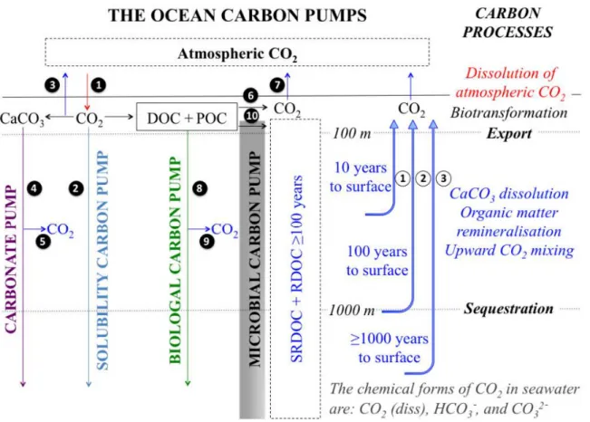
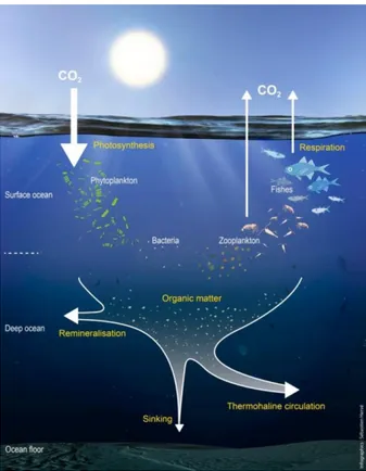
Figure 1.1: The four ocean carbon pumps. Figure from Legendre et al. (2015). Figure 1.2: Simplified view of the biological carbon pump (from S. Hervé, IUEM).
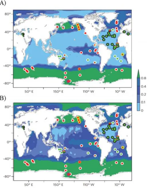
Figure 1.3: Patterns of nutrient limitation with backgrounds indicating the annual averages surface concentrations of A) nitrate (scaled by the mean N:P ratio of organic matter, i.e. 16) and B) phosphate in µmol L-1. From Moore et al., (2013).
Figure 1.4: Figure illustrating the major sources (in blue) and processes (in red) influencing the distribution of the TEIs. From GEOTRACES Science Plan.
Figure 1.5: The GEOTRACES plan, the black lines symbolizing the cruises completed during the international polar year, the yellow lines cruises completed and the red lines, cruises to be done. Map from the GEOTRACES website (www.geotraces.org).
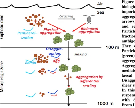
Figure 1.6: The components of particulate and dissolved iron pools (including the soluble and colloidal components) and the role of inorganic and organic components (adapted from Tagliabue et al., 2017). Figure 1.7: Schematic depiction of the biological carbon pump, emphasizing the important particle dynamics processes. From Lam and Marchal (2015).
Figure 1.8: Schematic of iron-binding ligand cycling in the ocean. From Buck et al. (2016).
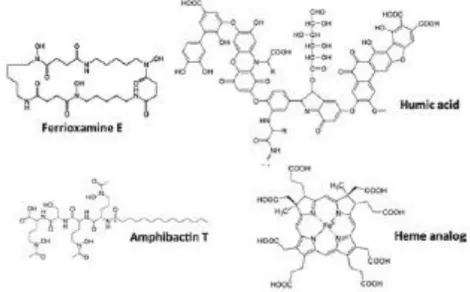
Figure 1.9: Examples of organic-iron binding ligand identities in seawater. The heme analog is siroheme, a relatively soluble iron-containing heme complex. From Buck et al. (2016).
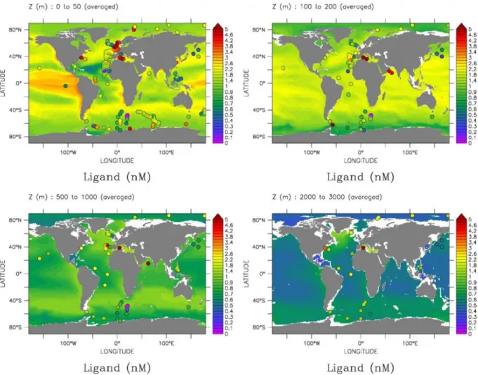
Figure 1.10: Ligand distribution as determined by the model of Völker and Tagliabue (2015) and in-situ measurements plotted as dots using the same color coding.
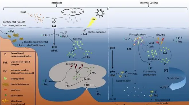
Figure 1.11: A revised representation of the major processes in the ocean iron cycle, with emphasis on the Atlantic Ocean. From Tagliabue et al. (2017).
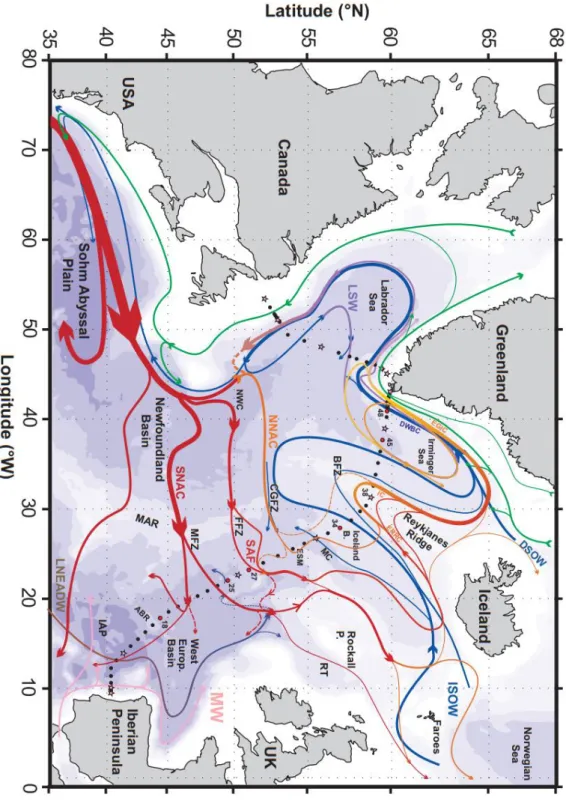
Figure 1.12: Map of the circulation scheme, the major topographical features, main basins, currents and main water masses of the North Atlantic Ocean. From Daniault et al. (2016).
Figure 1.13: Schematic of the geostrophic circulation over and around the Kerguelen Plateau during KEOPS. From Park et al. (2008b).
Figure 2.1: Historical perspective of the change in the range and average concentrations of dissolved Fe in the open ocean. From Blain and Tagliabue (2016).
Figure 2.2: Map of the GEOTRACES GA01 voyage track plotted on bathymetry as well as the major topographical features and main basins.
Figure 2.3: Pictures (from Helene Planquette) of (from the left to the right) Trace Metal Clean Rosette, Marie Cheize and Julia Boutorh sampling for trace metals and acidifying samples, 0.45 µm polyethersulfone filters (Supor®).
Figure 2.4: Location of the stations sampled during the HEOBI voyage using the Trace Metal Clean Rosette (modified from Thomas Holmes).
Figure 2.5: Pictures (from Peter Harmsen) of (from the left to the right) Kathrin Wuttig, the Trace Metal Clean Rosette in its protective coat before deployment, Andy R. Bowie and Manon Tonnard; Zanna Chase and Manon Tonnard sampling for trace metals through 0.2 µm Pall Acropak (Supor®) capsule filters.
Figure 2.6: Schematic of the off-line flow injection systems used at the IMAS showing solution flow paths during A) filling of sample and buffer loops, B) loading of buffered sample onto the column, C) column rinsing and conditioning, and D) elution of trace metals (modified from Rapp et al., 2017).
Figure 2.7: Schematic of the voltammetric cell and electrochemical process involved during analysis (modified from Cheize, 2012).
Figure 2.8: Schematics of A) potential variation at the working electrode surface as a function of time during the adsorptive cathodic stripping voltammetry (adapted from Wang, 2006), B) sample preparation before analysis, C) plot of the current intensity as a function of the potential applied for different Fe standard addition and D) plot of the reduction peak height as a function of total Fe concentration for a UV-digested seawater and a seawater that contains natural Fe-binding organic ligands (adapted from Cheize, 2012).
Figure 2.9: Distribution of the groups determined on the output of a Principal Component Analysis. Figure 3.1: Map of the GEOTRACES GA01 voyage plotted on bathymetry as well as the major topographical features and main basins.
Figure 3.2: Parameters measured from the regular CTD cast represented as a function of depth for GA01 section for A) Dissolved Oxygen (O2, µmol kg-1), B) Salinity and C) Temperature (°C).
Figure 3.3: Contour plot of the distribution of dissolved iron (DFe) concentrations in nmol L-1 along the GA01 voyage transect: upper 1000 m (top) and full depth range (bottom).
Figure 3.4: Vertical profiles of dissolved iron (DFe, black dots, solid line), particulate iron (PFe, black open dots, dashed line, Gourain et al., in prep.) and dissolved aluminium (DAl, grey dots, Menzel Barraqueta et al., 2018) at Stations 2 (A), and 4 (B) located above the Iberian shelf, Station 56 (C), Stations 53 (D) 53 and Station 61 (E) located above the Greenland shelf and Station 78 (F) located above the Newfoundland shelf.
Figure 3.5: Plot of dissolved iron (DFe, black circles) and dissolved aluminium (DAl, white circles, Menzel Barraqueta et al., 2018) along the salinity gradient between stations 1, 2, 4, 11 and 13 with linear regression equations.
Figure 3.6: Plot of dissolved Fe (DFe) Turnover Times relative to Atmospheric Deposition (TTADs) calculated from soluble Fe contained in aerosols estimated from a two-stage sequential leach (UHP water, then 25% HAc, Shelley et al., this issue).
Figure 3.7: Section plot of the Fe* tracer in the North Atlantic Ocean with a remineralization rate (RFe:N) of 0.05 mmol mol-1 from surface to 225 m depth.
Figure 4.1: A) Map of the GEOTRACES GA01 voyage track plotted on bathymetry as well as the major topographical features and main basins. B) Satellite Chlorophyll-a concentrations (MODIS Aqua from http://oceancolor.gsfc.nasa.gov), in units of mg m-3, before and during the GEOVIDE voyage (from March to June 2014). C) Contour plot of the measured total chlorophyll-a concentrations (TChl-a, mg m -3) for the GEOVIDE voyage transect.
Figure 4.2: The section represents the whole voyage track from station 2 to station 78 (total of 33 stations, note that stations 44 and 46 occupied the same location). Parameters collected from the regular CTD cast: temperature (A), salinity (B), dissolved O2 (C) and pH at 25°C (D) are represented as a function of depth. Figure 4.3: The section represents the whole voyage track from station 2 to station 78 (total of 33 stations). Nutrients collected from the regular CTD cast [Si(OH)4 (A), NO2- (B), NOx = NO2- + NO3- (C)], and from the Trace Metal Rosette (TMR) cast [DFe (D)] are represented as a function of depth.
Figure 4.4: Dissolved macronutrient (NOx, Si(OH)4) ratio (i.e. NOx:Si(OH)4) as a function of depth. Figure 4.5: GEOVIDE voyage cross sections of in situ TChl-a concentrations in mg m-3 (A-C) and percentages (D-F) associated to the pico-, nano-, and micro-phytoplankton size classes using Uitz et al. (2006) formulae.
Figure 4.6: A) Plot of integrated total Chlorophyll-a (TChl-a) concentrations (in green, from 0 to 150 m depth) along the GEOVIDE section. B) Stacked bars averaged per basins and depth range (0-25: from 0 to 25, 25-50: from 25 to 50, 50-100: from 50 to 100 m and 100-200: from 100 to 200 m depth) of the
Figure 4.7: Box and whisker diagram averaged per basins (0-200 m depth) (A) and stacked bars averaged per basins and depth range (0-25: from 0 to 25, 25-50: from 25 to 50, 50-100: from 50 to 100 m and 100-200: from 100 to 200 m depth) (B) of the percentage of the main phytoplankton classes as determined by CHEMTAX. Note that the colour coding is common to both plots.
Figure 4.8: Comparison between the phytoplankton size class as determine by CHEMTAX and by Uitz et al. (2006) formulae for the micro-phytoplankton (A), the nano-phytoplankton (B) and the pico-phytoplankton (C).
Figure 4.9: Sections of the tracers Si* (A) and Fe* (B) represented as a function of depth. Negative values indicate potential growth limiting nutrients while positive values indicate an excess of Si(OH)4 or DFe after complete biological uptake of NO3-.
Figure 4.10: Relationship between the Chl-a concentration integrated from 0 to 150 m depth and the fraction of A) micro-phytoplankton, B) nano- and pico-phytoplankton, C) nano-phytoplankton and D) pico-phytoplankton.
Figure 4.11: Plots of canonical correspondence analysis (CCA) and Pearson correlation with level of significance (i.e. ***, p-value < 0.001; **, p-value = [0.001 ; 0.01]; *, p-value = [0.01 ; 0.05]) for A) nutrients (NO3-, NO2-, Si and DFe) defined as objects and physical (salinity, temperature and pH) and biological (fractions of pico-, nano-, and micro-phytoplankton) parameters; and phytoplankton functional-classes (Diatoms, Dinophytes, Pelagophytes, Haptophytes-6, Haptophytes-8, Cryptophytes, Cyanobacteria, Prasinophytes and Chlorohytes) defined as objects with nutrients (NO3-, NO2-, Si, DFe, Si*, Fe*, NOx:Si) and physical (salinity, temperature, pH and z:Zeu) parameters for B) the NASTE province (stations 1-19), C) the NADR province (stations 19-38) and D) the ARCT province (stations 40-78).
Figure 4.12: Histograms of fractional drawdown ((winter – spring)/winter) of NO3- and Si for A) winter mixed layer depth and C) spring mixed layer depth and histograms of NO3-:Si ratios for B) winter mixed layer depth and D) summer mixed layer depth, for stations 1 to 19 located at the Iberian Margin and within the eastern part of the West European Basin. Black dashed line represents the optimal diatom N:Si uptake ratio.
Figure 4.13: Schematic of the potential limitations of the spring bloom in the North Atlantic Ocean along the GEOVIDE section.
Figure 5.1: Schematic of total chlorophyll-a (TChl-a) concentrations (green) at the sampling period of the HEOBI voyage on top of the main circulation features as in Park et al. (2008b) (D. Alain and S. Hervé, IUEM).
Figure 5.2: Section plots along the B-transect for A) potential temperature (θ), B) salinity and C) dissolved oxygen (O2).
Figure 5.3: The partitioning (when available) of iron (Fe) and Fe-binding organic ligand characteristics in the dissolved (DFe, <0.2 µm, solid circles and lines, data from Holmes et al., in prep.), soluble (SFe, <10 kDa, open circles, solid lines), and colloidal (CFe, 10 kDa – 0.2 µm, open circles, dashed lines) as a function of depth for A) the reference R18, B) B-transect B9, C) Heard Island H23 and D) McDonald Island M25.
Figure 5.4: Linear relationships between A) dissolved iron (DFe, data from Holmes et al., in prep.) and soluble Fe (SFe) concentrations, B) inorganic DFe and SFe (DFe’ and SFe’, respectively) and C) SFe and the reactivity of DLt (log α).
Figure 5.5: Box and whisker diagram of A) Fe concentrations (data from Holmes et al., in prep.), B) total Fe-binding organic ligand concentrations (Lt), C) the reactivity of Lt (log α), D) the inorganic Fe concentrations (Fe’) and E) the conditional stability constant (log K’, with respect to Fe3+) for the dissolved Fe fraction, and F) the fluorescence (in units of mg TChl-a m-3), G) silicates (μmol L-1), H) nitrates (μmol L-1), I) dissolved manganese (in nmol kg-1) data from Wuttig et al., in prep.) and J) Apparent Oxygen Utilization (AOU, (μmol kg-1)), as a function of the different water masses determined at the B-transect.
Figure 5.6: Plot of A) dissolved iron (DFe), B) Fe-binding organic ligand (Lt), C) conditional stability constant (log K’) and D) reactivity of Lt (log) as a function of depth for B9 from this study and B5 from Gerringa et al. (2008).
Figure 5.7: Box and whisker diagram of A) iron (Fe) concentrations, B) total Fe-binding organic ligand concentrations (Lt), C) conditional stability constants (log K’, with respect to Fe3+
), D) the reactivity of ligands (log α), E) excess Fe-binding organic ligands (L’), F) [L’]:[Fe] ratio, G) inorganic Fe (Fe’), and H) the percentage of Fe bound to Fe-binding organic ligands, and G) as a function of Fe fractions D (dissolved) C (colloidal) and S (soluble) for the B-transect (in blue), the reference stations (in green), Heard Island (in yellow) and McDonald Island (in purple).
Figure 5.8: Conceptual schematic of the main finding at Heard and McDonald Islands stations and the B-transect and R18 stations (D. Alain and S. Hervé, IUEM). (DFe data from Holmes et al., in prep., PFe data from van der Merwe et al., in prep.; pigment data from Wojtasiewicz et al., in prep., bacteria picture courtesy from S. Blain).
Figure 6.1 : Scatter plot of stations sampled in the West European Basin (purple), in the Iceland Basin (blue), in the Irminger Sea (green) and in the Labrador Sea (red) from past studies (open circles) and this study (triangles).
Figure 6.2: A) Map of the GEOTRACES GA01 voyage plotted on bathymetry as well as the major topographical features, main basins and corresponding Longhurst provinces. B) Summary of DFe supplies, main phytoplankton classes and potential limitation(s) within the North Atlantic Ocean.
Figure 6.3: A) Location of the stations sampled during the HEOBI voyage using the Trace Metal Clean Rosette (modified from Thomas Holmes). B) Conceptual schematic of the main finding at Heard and McDonald Islands stations and the B-transect and R18 stations (D. Alain and S. Hervé, IUEM). (DFe data from Holmes et al., in prep., PFe data from van der Merwe et al., in prep.; pigment data from Wojtasiewicz et al., in prep., bacteria picture courtesy from S. Blain).
Figure 6.4: Idea of an experimental setup for on-board incubations amended with aerosols and margin particles.
List of tables
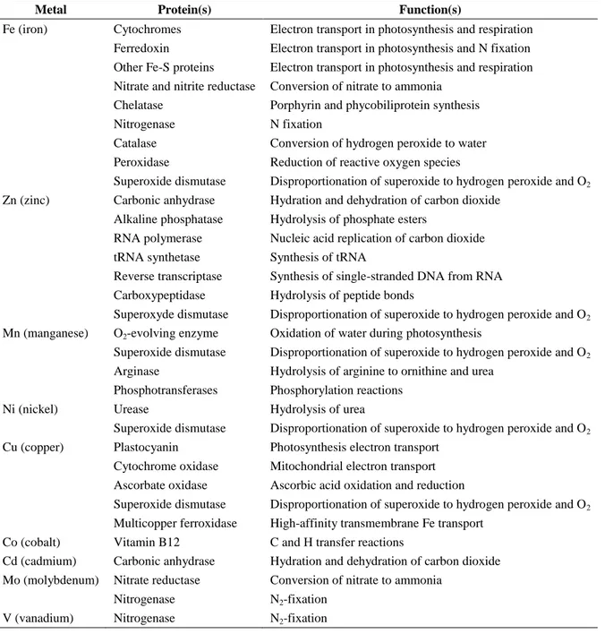
Table 1.1: Common metalloproteins present within marine phytoplankton. Adapted from Twining and Baines (2013).
Table 2.1: SAFe S, GSP and NASS-7 dissolved iron concentrations (DFe, nmol L-1) determined by the SeaFAST-picoTM and their consensus (SAFe S, GSP) and certified (NASS-7) DFe concentrations.
Table 2.2: SAFe S, SAFe D1, GSP, GSC and NASS-6 dissolved iron concentrations (DFe, nmol L-1) determined by the SeaFAST-picoTM and their consensus (SAFe S, SAFe D1, GSP, GSC) and certified (NASS-6) DFe concentrations.
Table 2.3: Metric performances of the HPLC analysis.
Table 2.4: Selection of pigments and their associated taxonomic significance for the CHEMTAX model. Table 2.5: Literature review referring all works realized in the covered area within the North Atlantic Ocean, special attention was given to studies using CHEMTAX method.
Table 2.6: Initial pigment ratio matrices [F0] for CHEMTAX model.
Table 2.7: Output matrices for the seven different groups determined by a Principal Component Analysis (PCA) from the CHEMTAX model.
Table 3.1: Station number, date of sampling (in the DD/MM/YYYY format), size pore used for filtration (µm), station location, mixed layer depth (m) and associated average dissolved iron (DFe) concentrations, standard deviation and number of samples during the GEOTRACES GA01 transect.
Table 3.2: SAFe S, GSP and NASS-7 dissolved iron concentrations (DFe, nmol L-1) determined by the SeaFAST-picoTM and their consensus (SAFe S, GSP) and certified (NASS-7) DFe concentrations.
Table 3.3: Averaged DFe:DAl (Menzel Barraqueta et al., 2018) and PFe:PAl (Gourain et al., in prep.) ratios reported per margins below 100 m depth.
Table 5.1: Concentrations of soluble iron (SFe), colloidal Fe (CFe), dissolved Fe (DFe, data from Holmes et al., in prep.), total particulate Fe (PFe, data from Van der Merwe et al., in prep.), and SFe:DFe, CFe:DFe, SFe:CFe, PFe labile:PFetotal, DFe:PFe ratios for the reference station and stations located nearby McDonald and Heard Islands.
Table 5.2: Median concentrations of soluble, colloidal and dissolved Fe, total Fe-binding organic ligands (Lt), [Lt]:[Fe] ratios, the conditional stability constant of Lt (log K’, with respect to Fe3+
), the reactivity of Lt (log α), inorganic Fe (Fe’), and the percentage of Fe bound to Lt for the reference, B-transect, Heard Island and McDonald Island stations and for different depth ranges.
Table 5.3: Comparison of median ligand characteristics for the different water masses determined for the B-transect (t-test).
Table 5.4: Comparison of median ligand characteristics within A) the dissolved, B) the colloidal and C) the soluble fractions for the four different areas when data were available, i.e. the reference station, the B-transect stations, Heard Island stations and McDonald Island stations (t-test).
Chapter 1:
C
hapter 1:
G
eneral introduction
Table of Contents1.1 The physical carbon pump ... 34
1.2 The biological carbon pump ... 36
1.2.1 Photosynthesis... 36
1.2.2 Carbonate counter pump ... 37
1.2.3 Phytoplankton bloom dynamic ... 38
1.2.4. Export of particulate organic matter ... 39
1.2.5. Remineralisation: grazing and microbial activity ... 40
1.2.6 Nutrient controls ... 41
1.2.6.1 Macronutrients ... 42
1.2.6.2 Micronutrients ... 43
1.2.6.3 Response of the phytoplankton community to the availability of nutrients ... 47
1.3. The GEOTRACES program ... 48
1.4. Physico-chemical speciation of Fe... 50
1.4.1 Physical speciation ... 50
1.4.1.1 Particulate pool ... 51
1.4.1.2 Dissolved pool ... 53
1.4.1.3 Soluble and colloidal pools ... 54
1.4.2 Chemical speciation ... 55
1.4.2.1 Redox speciation ... 55
1.4.2.2 Organic speciation ... 57
1.5.1 External sources of Fe ... 64
1.5.1.1 Atmospheric deposition... 64
1.5.1.2 Riverine inputs ... 66
1.5.1.3 Sediment inputs ... 66
1.5.1.4 Hydrothermalism ... 67
1.5.1.5 Glaciers, icebergs and melting sea ice ... 68
1.5.1.6 Submarine groundwater discharge ... 70
1.5.2 Regenerated sources of Fe ... 70
1.6 Summary of literature review ... 71
1.7 Study areas and thesis goals ... 72
1.7.1 The North Atlantic Ocean ... 72
1.7.2 The Kerguelen Plateau (Indian sector of the Southern Ocean)... 75
The estimated global oceanic carbon sink estimate is of 2.7 ± 0.5 PgC.yr-1 (Le Quéré et al., 2013), representing about 30% of annual atmospheric fuel emissions, highlighting the central role of the ocean in the global climatic system.
At the air-sea interface, the diffusion of atmospheric CO2 in the ocean is enhanced by the difference of CO2 partial pressure (ΔpCO2) between the ocean and the atmosphere. The solubility and distribution of the CO2 within the oceans depend not only on many physico-chemical factors such as temperature, salinity or the turbulence regime, but also on biotic factors (photosynthesis, calcification). Once the CO2 is dissolved within surface waters, it is then transported horizontally and vertically throughout the oceanic layers by three main processes i) the physical carbon pump, ii) the organic carbon pump and iii) the carbonate counter pump (Volk and Hoffert, 1985), the two last processes being gathered under the name of the biological carbon pump. More recently, additional concepts such as the microbial carbon pump and the lithogenic carbon pump (not detailed here) have been introduced into this general scheme (Bressac et al., 2014; Legendre et al., 2015; Ternon et al., 2009). All these processes are responsible for the heterogeneous vertical distribution of DIC in the ocean that results in a strong gradient of approximately 300 µmol kg-1 between the surface and the deep ocean.
1.1 The physical carbon pump
The physical carbon pump includes two physico-chemical processes:
- the adsorption of CO2 at the air-sea interface controlled by a thermodynamic equilibrium (i.e. the solubility pump) and
- its vertical transport in the ocean through the global thermohaline circulation.
Once in seawater, the atmospheric gaseous CO2 is transformed into dissolved inorganic carbon (DIC), which includes the following forms: the non-dissociated form (CO2 aq), the carbonic acid (H2CO3, i.e. the hydrated form), the bicarbonate ions (HCO3-) and the carbonate ions (CO32-). CO2 is a weak acid and when it dissolves, it reacts with water to form carbonic acid, which dissociates following equations 1.1 and 1.2 (Denman et al., 2007).
( ) ( ) (eq. 1.1)
The CO2 absorption increases the ocean acidity by adding H+ ions in solution, which resulted in a decrease of the sea surface pH by about 0.1 pH units since the beginning of the industrial revolution (Caldeira and Wickett, 2003).
Figure 1.1: The four ocean carbon pumps: The solubility pump, i.e., the dissolution of atmospheric CO2 in surface waters (1), followed by deep mixing of the CO2-rich water and sequestration (2); The carbonate pump, i.e., the bio-precipitation of CaCO3 (or PIC) in the upper water column which is accompanied by the release of CO2 (3), followed by the sinking of bio-mineral particles to depth where their carbon is sequestered (4); The biological pump, i.e., the photosynthetic uptake of carbon by phytoplankton and its transformation by the food web in the euphotic zone, including respiration (6) and loss to the atmosphere (7), followed by transfer of particulate organic carbon (POC) into deep waters where it is sequestered (8). During the downward transit from 100 to 1000m, CO2 is released in the water column by dissolution of part of sinking CaCO3 (5) and remineralisation of part of the POC that is transferred to depth (9). The production of recalcitrant DOC (RDOC) and semi-refractory DOC (SRDOC) with a life time ≥ 100 years (i.e., DOC>100) presumably by microbial activity, will sequester ocean carbon because their lifetimes are ≥ 100 years (10). The small numbers in full circles identify arrows in the figure. Figure from Legendre et al. (2015).
The solubility pump is a mechanism that controls the adsorption or the outgassing of gaseous CO2 that is modulated by air-sea CO2 exchange as a function of CO2 solubility (itself an inverse function of temperature), the difference of CO2 partial pressure between the surface ocean and the atmosphere, and the gas transfer coefficient (Takahashi et al., 2002; Weiss, 1974). Cold and denser water masses from high latitudes sinks, then spreads at depth
formation takes place such as the Subpolar North Atlantic (Karleskind et al., 2011) and the Subantarctic Southern Ocean (Sallée et al., 2012). Warmer waters originating from low latitudes then compensate the water deficit at the surface. The coupling between CO2 adsorption and thermohaline circulation will transfer carbon to the deep ocean in cold areas of the globe while tropical areas will favour a degassing of CO2. The time scales to which the DIC is exchangeable with the atmosphere depend on the depth at which the DIC is transported via the circulation. Indeed, the DIC can be sequestered in the ocean from weeks in the surface to centuries at 3000 m depth.
1.2 The biological carbon pump
The biological pump is a suite of biologically mediated processes that consist of surface transformation of DIC into dissolved organic carbon (DOC) and particulate organic carbon (POC), with the subsequent sinking and remineralisation of this organic matter. The DOC oceanic stock is the net result of autotrophic production by marine phytoplankton and heterotrophic microbial remineralisation (Hansell, 2001) (Fig. 1.1).
The observed gradients of DIC and DOC highlight the fundamental role of biology in the vertical distribution of carbon stocks in the ocean, which determines the time scales over which oceanic and atmospheric reservoirs interact and thus partly regulates the atmospheric CO2 content (Kwon et al., 2009).
1.2.1 Photosynthesis
The biological carbon pump is governed by photosynthesis processes realized by micro-organisms, including all photo-autotroph planktonic organisms, mainly unicellular (Falkowski et al., 2003) convert the DIC and dissolved mineral matter into particulate organic matter (POM, e.g. sugars) and biominerals (e.g. calcite, CaCO3, for coccolithophores; opal, BSiO2, for diatoms). This carbon fixation, also defined as primary production (PP), fuels the flux of POC and is limited by the availability of light and nutrients and thus only occurs in ocean where solar radiation penetrates (i.e. the euphotic layer) (eq. 1.3, Fig. 1.2).
→ ( )
( ) ( ) (eq. 1.3)
Figure 1.2: Simplified view of the biological carbon pump (from S. Hervé, IUEM).
In the absence of the biological carbon pump, atmospheric CO2 concentration would increase by approximately 50% (200 ppmv, e.g. Boyd, 2015; Parekh et al., 2006; Sanders et al., 2014), a considerable fraction compared to present days ~ 400 ppmv. Therefore, through the biological carbon pump, ocean plays a key role in the functioning of the carbon cycle at the global scale.
1.2.2 Carbonate counter pump
Another important process that removes DIC within the upper layer of the water column involves the formation of PIC via the precipitation of CaCO3 (eq. 1.4). Many species through a broad range of trophic levels are able to precipitate CaCO3 (e.g. calcite or aragonite) in order to form a protective coating or shell, including some phytoplankton taxa such as coccolithophorid cells and calcareous dinophytes as well as other marine organisms (corals, foraminifera, mollusk and crustacean). However, when the PIC is exported to the deep ocean, i.e. below the lysocline, it dissolves, being responsible for a third of the vertical DIC gradient.
Although the calcification process in the mixed layer decreases DIC and therefore alkalinity, it is counter balanced by the production of carbonic acid, which increases the concentration of CO2 in seawater initiating a diffusive flux of CO2 from the ocean to the atmosphere (Frankignoulle et al., 1994) (eq. 1.4). Estimations of switching-off the calcification in the ocean suggest that it would lead to a 40 ppmv decrease in atmospheric pCO2 (Wolf-Gladrow et al., 1999). However, in calcium carbonate dominated regions, a higher fraction of the organic matter is exported to the deep ocean ballasted by the CaCO3 (Francois et al., 2002).
1.2.3 Phytoplankton bloom dynamic
Sverdrup (1953) suggested that blooms are caused by enhanced growth rates in response to improved light, temperature, stratification conditions and availability of nutrients because of winter mixing thus enabling the initiation of the spring bloom. The first phytoplankton organisms to take advantage of such conditions and to bloom are the micro-phytoplankton, which are then succeeded by a mixture of size-classes and functional groups depending of the resources. The bloom termination will thus result from nutrient depletion, higher grazing pressure and/or decreasing light quality.
Although the critical depth hypothesis explains the spring-summer bloom, it does not explain the vernal bloom. Several hypotheses have been advanced. For example, Behrenfeld (2010) reported that winter physical forcing could modulate the prey-predator relationship via the deepening of the Mixed Layer Depth (MLD) that dilutes phytoplankton in a higher volume and thus limits zooplankton predation rate. This dilution-recoupling hypothesis can thus explain a vernal accumulation of the phytoplankton biomass. Furthermore, Lindemann and St. John (2014) highlighted that phytoplankton have the ability to regulate their respiration rate to obscurity, which will thus reduce losses within the vernal mixed layer. As a result, there is no relationship between the accumulation rate and the growth rate, as biomass can accumulate within deep mixed layer despite a low growth rate. Physical processes such as meso- and sub-mesoscale features (i.e. eddies, upwellings, fronts) can also greatly influence the bloom dynamic by restratification of the deep mixed layer within a timescale of days while the heat fluxes are still negative (Boccaletti et al., 2007; Fox-Kemper et al., 2008). Indeed, eddies developing within horizontal density gradients could lead to the horizontal transport of denser water masses under lighter water masses, which thus stays at the surface. Similarly, wind can also strengthen or lower the restratification through the Ekman transport (Mahadevan et al., 2010).
Diffusion and advection can reintroduce nutrients in the euphotic layer and fuel the primary production (Benitez-Nelson et al., 2000). Lacour et al. (in prep.) reported that the alternation between convective mixing and restratification could lead to episodic carbon export of organic matter produced in surface resulting from the remnant layer, which is the layer included between the depth of a recent mixing and the depth of a past mixing. All these different features that either bring pulses of new nutrients towards the euphotic layer and the dynamic of the mixed layer, explain part of the spatial variability of phytoplankton biomass (Mahadevan et al., 2012; McGillicuddy et al., 2003) and of POC export (Guieu, 2005; Karleskind et al., 2011; Waite et al., 2016).
1.2.4. Export of particulate organic matter
POC and more generally, POM, generated through primary production becomes available for the heterotroph oceanic ecosystem. It constitutes the basis of the marine trophic web and it is further exported towards the deep ocean as dead organisms and faecal pellets sink. The magnitude of the POM export and therefore of the associated nutrients depends on many parameters: 1) The nutrient availability that will drive part of the bloom magnitude and the taxonomic composition of the phytoplankton community, 2) the amount of suspended biomineral and lithogenic particles, 3) organic particles (other than phytoplankton cells) excreted by either phytoplankton, bacteria or higher trophic levels as faeces.
The size structure of the phytoplankton community with higher export related to greater size of sinking phytoplankton cells (Alldredge and Silver, 1988; Guidi et al., 2009) and the density and shape of the phytoplankton cells have been shown to influence the efficiency of the POM export (Klaas and Archer, 2002). Indeed, incorporation of biogenic silica (BSiO2) or calcite (CaCO3) into aggregates increases the excess density of suspended particles leading to higher sinking velocity (Honjo, 1996) with a faster transfer to deep ocean when POM is ballasted by calcite (Francois et al., 2002). However, due to their important density relative to seawater, these organisms, especially diatoms, increase their surface area relative to their volume to slow their export and to remain suspended for a longer time in the euphotic layer. Although, non-silicified and non-calcified organisms are barely heavier than seawater (~1.05 g cm-3), such adaptive strategies are not limited to silicifying organisms (Padisák et al., 2003). An additional process that affect the POM export is the amount of terrigenous material (e.g. dust, clays), which ballast effect is intermediate compared to CaCO3 and BSiO2 or even lower than BSiO2 and greatly depends on the sources and