Do the time-wrap: continuous alignment of gene expression time-series data

Do the Time-Warp: Continuous Alignment of Gene

Expression Time-Series Data

by

Georg Kurt Gerber

B.A., Mathematics, UC Berkeley (1991) M.P.H., Infectious Diseases, UC Berkeley (1994)

Submitted to the Department of Electrical Engineering and Computer Science in partial fulfillment of the requirements for the degree of

Master of Science in Electrical Engineering and Computer Science at the

MASSACHUSETTS INSTITUTE OF TECHNOLOGY

Author.

February 2003

©

Massachusetts Institute of Technology 2003. All rights reserved.

...

/Departpnt of Electrical Engineering and Computer Science September 1, 2002

C ertified by ... ... David K. Gifford Professor of Electrical Engineering and Computer Science Thesis Supervisor

Accepted by...

Arthur C. Smith Chairman, Department Committee on Graduate Students

MASSACHUSETTS INSTITUTE

OF TECHNOLOGY

Do the Time-Warp: Continuous Alignment of Gene Expression

Time-Series Data

by

Georg Kurt Gerber

Submitted to the Department of Electrical Engineering and Computer Science on September 1, 2002, in partial fulfillment of the

requirements for the degree of

Master of Science in Electrical Engineering and Computer Science

Abstract

Recent advances in DNA microarray technologies are enabling researchers to measure the expression levels of thousands of genes simultaneously, with time-series data offering par-ticularly rich opportunities for understanding dynamic biological processes. Unfortunately, DNA microarray data is plagued by quality issues including noise and missing data points. Expression time-series data introduce additional complications, including sampling rate dif-ferences between experiments and variations in the timing of biological processes.

In this thesis, a probabilistic framework is presented for making gene expression time-series data from different experiments directly comparable. This method addresses the issues of DNA microarray data noise, missing values, different sampling rates between experiments, and variability in the timing of biological processes. Gene expression time-series data are represented as a set of continuous spline curves (piecewise polynomials) using a linear mixed-effects model, a statistical method that allows for a fixed or group effect as well as a random or individual effect. The model constrains a gene's expression curve to be generally similar to those of co-expressed genes, while still allowing for gene specific variations. A continuous alignment algorithm is then introduced in which a search is performed for a function that transforms the time-scale of one gene expression process into that of another, while minimizing a measure of error between expression profiles in the two processes.

Three applications are then presented of the continuous representation/alignment al-gorithm to DNA microarray expression data, which yield biologically meaningful results. First, it is shown that the linear mixed-effects spline model can effectively predict missing data values, achieving lower error for cases of one or two consecutive missing values than the best method previously reported in the literature. Second, it is demonstrated that the alignment algorithm can produce stable low-error alignments, allowing data from three different yeast cell cycle experiments (with period and phase differences) to be combined. Finally, it is shown that the alignment algorithm can be used to identify genes that behave differently in normal versus genetically modified cells.

Thesis Supervisor: David K. Gifford

Biographical Information

Personal

Born: December 31, 1970 in Los Angeles, CA.

Education

B.A., Mathematics, summa cum laude, UC Berkeley, 1991. M.P.H., Infectious Diseases, UC Berkeley, 1994.

Work Experience

" Graduate Research Assistant, M.I.T. Laboratory for Computer Science (Supervisor: Prof. David Gifford), 2000-present.

" Instructor, Northeastern University Bioinformatics Essentials Graduate Certificate Program, 2002.

" Chief Technology Officer, IS?TV, Inc., 2000.

" Senior Vice President, L-Squared Entertainment, Inc., 1995-1999.

" President and Chief Executive Officer, Infinite Interactions, Inc., 1993-1995.

" Graduate Research Assistant, UC Berkeley Department of Computer Science (Super-visor: Prof. Brian Barsky), 1993-1994.

" Research Associate/Laboratory Automations Specialist, Metabolex, Inc., 1992. " Undergraduate Research Assistant, UC Berkeley Department of Biophysics

(Supervi-sor: Prof. Hans Bremermann), 1990.

" President, Speak Easy Communications System, 1984-1989.

Awards

" National Defense Science and Engineering Graduate (NDSEG) Fellowship (awarded and accepted), 2002.

" National Science Foundation (NSF) Fellowship (awarded), 2002. " University of California Regents' Graduate Fellowship, 1992-1994.

* UC Berkeley Highest Distinction in General Scholarship in Mathematics, 1991. " Phi Beta Kappa honor society, elected 1990.

" University of California Regents' Undergraduate Scholarship, 1989-1991. " UC Berkeley Dean's List, every semester attended, 1989-1991.

Acknowledgments

I must first thank Ziv-Bar Joseph, a fellow graduate student in my research group and collaborator on much of the work that led to this thesis. Ziv was instrumental in adapting the linear mixed-effects spline model for use on gene expression time-series data. He was also very helpful in many other aspects of this work, such as finding applications and coming up with validation techniques. Ziv has been more than just a great intellectual collaborator; he has been a true friend.

I must also acknowledge Professor David Gifford, my research supervisor. He first introduced me to the field of computational functional genomics and has been instrumental in encouraging my research by providing ideas, resources, and guidance while also fostering the critical collaborative relationships outside of our immediate group. Professor Gifford is one of those rare individual who possesses both the intellectual power and dedication needed to crack hard research problems, as well as the courage and entrepreneurial spirit needed to blaze trails in a new field.

Professor Tommi Jaakkola has also been critical in the development of this thesis. He first suggested applying mixed-effects spline models to gene expression data, and subse-quently provided insights and guidance throughout this entire research project. Professor Jaakkola's deep knowledge of statistics and machine learning has inspired my own interests in these subjects.

Professor Rick Young at the Whitehead Institute has provided much inspiration for the "biological half" of this thesis. His passion for biology and unlocking the secrets of genetic regulation is infectious. Professor Young has also been critical in fostering true collaborations between biologists in his lab and computer scientists in my group. I must specifically thank him for encouraging my relationship with Dr. Itamar Simon, a Post-Doctoral Researcher in the Young lab. Dr. Simon's work on the cell cycle genetic regulatory network provided much of the initial motivation for the algorithms presented in this thesis. He also suggested the application of the alignment algorithm to identifying genes that are differentially expressed in wildtype versus mutant cells.

Within my own research group, I must acknowledge fellow graduate students Reina Rie-mann, John Barnett, and Tim Danford for the many stimulating ideas about computational biology that they have shared with me. Reina Riemann, my office mate during my first year with the group, was particularly helpful in providing insights during the early stages of the work that led to this thesis. Jeanne Darling, Professor Gifford's secretary, is one of the most knowledgeable and helpful people I have encountered at M.I.T. (or anywhere else for that matter!) She has always been there to offer advice and to lend a helping hand as I have tried to find my way through the M.I.T. maze.

I would also like to acknowledge the memories of two teachers from my pre-M.I.T. days who were critical in my intellectual development. Professor Donald Mazukelli introduced me to the beauty of mathematics, giving me a life-long gift. Professor Hans Bremermann, one of the humblest and warmest people I have ever known, introduced me to the concept of trying to use equations to describe the behavior of living organisms, and in so doing, sparked my unrelenting passion for mathematical biology.

Finally, I must acknowledge my family, who started setting me on my intellectual path before I even knew it. My brother Karl grew up with me like a twin, and his determination and risk-taking spirit rubbed off on me. My older sister Margot has always supported my offbeat interests and encouraged me to think outside the box. Although my father Barry has never had much tolerance for moldering academics, since my earliest memories he has

always conveyed to me a great love of learning. He never separated me from "adult" ideas or tools, always letting me explore his books, computers, and electronic gadgets. Most importantly, he had the wisdom to do something incredibly hard: he resisted intruding too much in my explorations so that I could learn to think independently. My mother Jane sparked my curiosity and love for living things. When I was young, she spent endless hours reading books about dinosaurs and pre-historic people to me, radiating her sense of the mystery and beauty of the biological world. Years later, she revealed another trait - courage - when she fought a serious illness, and once again reminded me of just how

important life is.

Finally, I must acknowledge Anne-Marie (1995-2002), for being a part of my life for as long as she could. She was there throughout so much, both the happy and the sad: our days in Los Angeles when I worked as an executive in Hollywood, my mothers' illness, my difficult decision to re-enter the academic world, and our move across the country to Boston. I miss her very much, and will always remember the love and happy times we enjoyed together.

A Note on Notation

An effort has been made to use consistent notation throughout this thesis. Scalars will be denoted with italic Roman or Greek lower-case letters such as x and y or A. All vectors will be column vectors and denoted with bold italic Roman or Greek lower-case letters such as x and y or p. Matrices will be denoted with bold italic Roman or Greek upper-case letters such as A and B or r. Sets will be denoted with upper-case Roman italic letters such as C and T. Random variables will be denoted by fonts without serifs such as x and y for random scalars and x and y for random vectors. Unfortunately, lower-case Greek letters are also used for random variables but the sans serif style is not available. In these cases, the intention should be clear from the context.

"... he ended up recommending to all of them that they

leave Macondo, that they forget everything he had taught them

about the world and the human heart, that they shit on Horace,

and that wherever they might be they always remember that the

past was a lie, that memory has no return, that every spring

gone by could never be recovered, and that the wildest and most

tenacious love was an ephemeral truth in the end."

Contents

1

Introduction 17 1.1 Problem Description . . . . 17 1.2 Solution Overview . . . . 18 1.3 Thesis Roadm ap . . . . 19 1.4 Related W ork . . . . 20

2 A Probabilistic Model for Estimating Gene Expression Time-Series Data with Continuous Curves 23 2.1 Linear Mixed-Effects Models . . . . 24

2.2 The Expectation-Maximization (EM) Algorithm . . . . 26

2.3 Splines . . . . 27

2.3.1 B -splines . . . . 29

2.4 Gene Expression Time-Series Linear Mixed-Effects Spline Model . . . . 31

3 Aligning Continuous Gene Expression Time-Series Profiles 33 3.1 Alignment Framework . . . . 33

3.2 Alignment Error Measure . . . . 34

3.2.1 Alternate Weighting for the Error Measure for Knockout Experiments 35 3.3 Minimizing the Alignment Error Measure . . . . 35

3.4 Approaches for Speeding Up the Alignment Algorithm . . . . 36

4 Applications 39 4.1 Description of Data Sets Analyzed . . . . 39

4.2 Prediction of Missing Values. . . . . 41

4.3 Aligning Similar Biological Processes . . . . 43

4.4 Identifying Differentially Expressed Genes . . . . 45

5 Conclusion 49 5.1 Future W ork . . . . 49

A Overview of Molecular Genetics 51 A.1 Essential Molecules For Life: DNA, RNA and Proteins . . . . 51

A.2 Genes and Regulation . . . . 52

A.3 The "New Era" of Genomics . . . . 53

B DNA Microarrays 55 B.1 Photolithographic Oligonucleotide Arrays . . . . 55

B.3 Comparison of Photolithographic Oligonucleotide and Printed cDNA Arrays 57 B.4 Limitations of DNA Microarrays . . . . 57

C Derivations 59

C.1 Random Effects Predictor for the Linear Mixed-Effects Model . . . . 59 C.2 Estimating Parameters of the Linear Mixed-Effects Model Using the EM

A lgorithm . . . . 60 C.2.1 Modifications Necessary for the Gene Expression Time-Series Linear

Mixed-Effects Spline Model . . . . 62 C.3 Expanded Form of the Spline Predictor . . . . 63

List of Figures

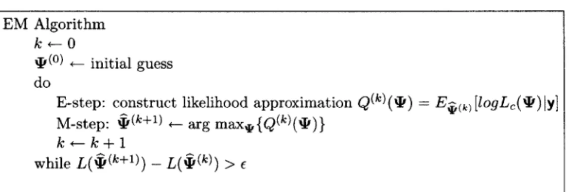
2-1 Pseudo-code for the Expectation-Maximization (EM) algorithm, a general method for iteratively computing maximum likelihood (ML) estimates. Here, %F is a vector of parameters to be estimated, L(%I) is the data likelihood function, Lc('I) is the complete data likelihood function, and

e

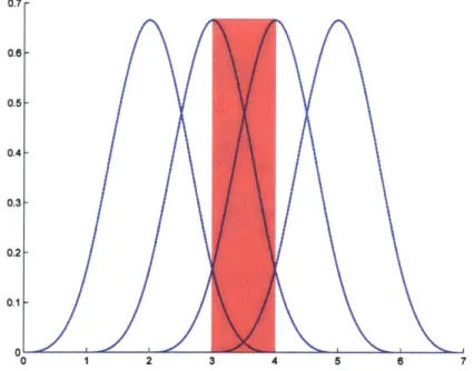
is a small numerical tolerance threshold. The algorithm proceeds by forming an esti-mate of the data likelihood function, by taking the conditional expectation of the complete data likelihood function with respect to the observed data and the current estimates of the parameter values (E-step). In the M-step, new parameter estimates are obtained by maximizing the likelihood of the estimated data likelihood function obtained in the previous E-step. .... 27

2-2 The B-spline basis functions are periodic (translates of one another) when a uniform knot vector is used. Shown here is the normalized cubic B-spline basis (k = 4) with knot vector x = (0, 1, 2, 3, 4, 5, 6, 7)T. Note that the B-spline will only be defined in the shaded region 3 < t < 4, where all four basis functions overlap . . . . 30

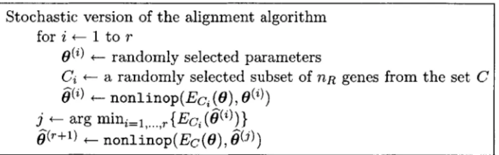
3-1 Pseudo-code for the stochastic version of the alignment algorithm, which is useful for reducing the running time of the alignment algorithm when a large number of genes are being processed. Here, r is a pre-specified number of random re-starts,

6

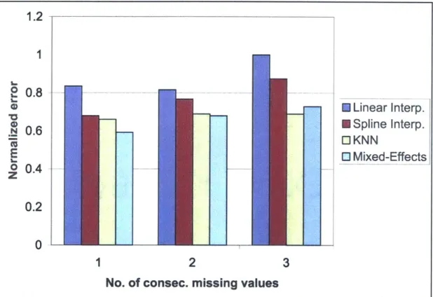
is a warping parameter vector, Ec(6) is an alignment error function over a set of genes C, and nonlinop(-, .) is a numerical con-strained non-linear optimization routine, where the second argument is the starting "guess" for the parameter vector. The algorithm begins by choos-ing a random subset of nR genes from the total set C of genes and random initial settings for the warping parameters from a uniform distribution. The minimization procedure as described in section 3.3 is then carried out and this process is repeated a fixed number of times, r, with a new random choice of initial warping parameters each time. Upon termination, the alignment parameters that corresponded to the lowest error are chosen. These parame-ters are then used as the starting values for the error minimization procedure using the full set of genes. . . . . 38

4-1 For predicting missing expression values, the linear mixed-effects spline method outperformed linear and standard spline interpolation in all cases, and was superior to K-nearest neighbors for the cases of one and two consecutive missing values. K-nearest neighbors (KNN) performed slightly better in the case of three consecutive missing values, but this case is fairly extreme and probably not likely to occur often in practice. The validation involved picking a gene at random from the data set and then removing one, two, and three consecutive time-points. Values for these time-points were then estimated us-ing all remainus-ing data and this process was repeated 100 times. A mean error was then computed for each case of one, two, or three consecutive missing data points. The errors shown were normalized by the largest error (linear interpolation with three consecutive missing values). The results shown were obtained using the cdc15DS . . . . 42 4-2 With the alignment algorithm it was estimated that the cdc28DS cell cycle

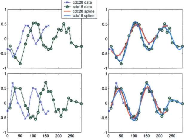
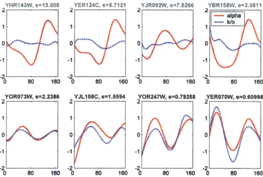
runs at ~ 1.4 times the speed of the cdc15DS cycle and starts ~ 5.5 minutes before, a biologically reasonable result. Linear warping was used with the full set of approximately 800 cell cycle regulated genes. The left-hand side shows averages of unaligned expression values for genes in one of two phase classes. The right-hand side shows averages of the aligned predicted spline curves (and averages of the expression data values) for genes in one of two phase classes. The top row shows the G1 phase class (186 genes), and the bottom row the S/G2 phase class (283 genes). . . . . 47 4-3 Genes that are regulated by Fkh2 can be identified by first aligning the

Fkhl/2 knockout and the wildtype alpha mating factor synchronized data sets, and then ranking genes determined to be bound by Fkh2 (in a DNA-binding assay) according to their alignment error scores. Shown are the genes with the four worst (top row) and best (bottom row) alignment scores. A poor alignment score indicates that a gene is behaving differently in the knockout than it is in the wildtype experiment. See text for biological interpretation of these results. . . . . 48

List of Tables

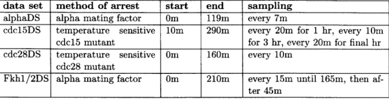
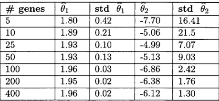
4.1 Summary of the four publicly available gene expression time-series data sets analyzed in this thesis. The first three data sets are from the work of Spell-man et al [51], in which yeast cells were synchronized using three different methods. The fourth data set is from a study by Zhu et al [60], in which the genes fkhl and fkh2, encoding transcriptional regulators, were knocked out. 41 4.2 The estimated alignment parameters for the alphaDS to cdc15DS registration

exhibit low variances even when fairly small sets of genes are used. Shown are the results of experiments in which random subsets of fixed size were sampled 100 times and alignment of the alphaDS to the cdc15DS was performed, using a linear warping function. The columns are as follows: number of genes used, stretch/squash parameter, standard deviation of this parameter, translation parameter, and standard deviation of this parameter. Note that the variance in the parameters decreases as more genes are used and there is convergence to the O1 = 1.95 and 2 = -5.89 settings found using the full set of genes. . 44

Chapter 1

Introduction

1.1

Problem Description

Recent advances in DNA microarray technologies are enabling researchers to measure the expression levels of thousands of genes simultaneously. These technologies are proving invaluable in functional genomics, a developing field in which investigators ultimately seek to understand genetic activity at the level of an organism's entire collection of genes [25]. Time-series expression data, the focus of this thesis, offer particularly rich opportunities for understanding dynamic biological processes such as the cell cycle, development, and immune response [51, 57, 38].

Two common analytical objectives in functional genomics are, 1) identifying genes that behave differently under alternate experimental conditions and, 2) building networks of genetic interactions. In the first case, researchers may be interested in determining which genes are affected by an experimental intervention such as a gene knockout [60], or they may want to identify genes whose expression patterns are altered during a natural pathological process such as cancer [4]. The goal in such experiments is to identify significant differences between gene expression in a "normal" versus an alternate condition. In the second type of analysis, researchers seek to construct networks of genetic interactions and to understand complexities of these system, such as the role of combinatorial regulation or feedback loops. Given the scale and the complexity of the biological systems being studied, sophisticated computational techniques such as Bayesian Networks have been employed [19, 21, 22].

Unfortunately, DNA microarray data are plagued with quality issues that make both of the above mentioned analyses challenging. Large amounts of noise may be introduced dur-ing the many steps of sample preparation, hybridization, and detection. Further, in some experiments expression data points for a given gene may be "missing", due to practical difficulties such as detergent bubbles on glass slides or manufacturing defects in the mi-croarray [23]. For these reasons, a large literature has developed describing computational and experimental methods for dealing with the noise inherent in DNA microarray data (see for instance [26, 54, 12, 29, 13]). However, few of these methods address the specific features of temporal microarray data.

On the one hand, gene expression time-series data provide information lacking in static data that can be useful in overcoming noise and missing value problems. For instance, it should be possible to exploit the reasonable assumptions that adjacent time points will be statistically dependent on one another, and that expression values will vary fairly smoothly with time. On the other hand, gene expression time-series data introduce two complications

not present in static analyses: lack of standard sampling rates and variability in the timing of biological processes.

The first issue is a practical one: since DNA microarrays are expensive and time-series experiments are often technically challenging to perform, biologists want to sample a min-imum number of time-points. Unfortunately, there is a dearth of empirical or theoretical information on appropriate sampling rates, since large-scale gene expression time-series ex-periments are a relatively new phenomena. This has resulted in published DNA microarray studies of the same or similar biological processes sampled at very different time-points. Non-uniform sampling or coverage of different portions of the process add to the difficulties in comparing data sets.

The second issue is a biological one: the rate at which similar underlying processes unfold can be expected to differ across organisms, genetic variants and environmental conditions. For instance, extensive gene expression time-series data has been collected to study the yeast cell cycle [51]. In these experiments, different methods have been used to synchronize the cells, and these have resulted in variations in growth rates and other aspects of the cell cycle. Thus, while the data sets collected capture the same fundamental process, the phases and periods of the expression levels of cell cycle genes differ markedly between the experiments.

When analyzing time-series data for the objectives of identifying differentially expressed genes and building genetic networks, one must address both the issue of different sampling rates between experiments and that of biological variability in the timing of processes. In the case of identifying differentially expressed genes, one would like to analyze data from the two conditions on the same time-scale so that direct comparisons can be made. For the second objective of building genetic networks, the statistical models often used require large amounts of data. One would like to combine as much data measuring the same or similar biological processes as possible. Thus, for both analytical objectives one would like a computational method for making gene expression time-series data from different experiments directly comparable. Further, the method should exploit the special structure of time-series data to deal with the general problems of DNA microarray data - noise and missing data points.

1.2

Solution Overview

In this thesis, a probabilistic framework will be presented for making gene expression time-series data from different experiments directly comparable. This method addresses the issues of DNA microarray data noise, missing values, different sampling rates between experiments, and variability in the timing of biological processes. Gene expression time-series data are represented as a set of continuous curves whose time-scales can be smoothly warped so as to align different data sets. Splines or piecewise polynomials are a natural tool for estimating such smooth curves. However, given the noise and missing value problems inherent in DNA microarray data, fitting an independent spline to each gene's expression pattern can be problematic. Fortunately, biology can help: it has been demonstrated that genes involved in similar processes often do not behave independently [15]. Such genes are said to be co-expressed, and can be identified using previous biological knowledge or clustering algorithms. The expression profiles of co-expressed genes can be assumed to be statistically dependent on one another, but aren't expected to be identical. For instance, co-expressed genes might be expected to peak at approximately the same time, but the magnitudes of the peaks could

differ somewhat.

The statistical model presented in this thesis uses co-expression information to constrain the shape of a gene's expression profile (spline) to be generally similar to those of co-expressed genes, while still allowing for gene specific variations. Further, these similarity constraints are lessened when more information is available, i.e., there are a large number of data points for a gene's expression time-series. The type of model used is a linear mixed-effects model, which assumes that observations of a given random variable can be explained as a combination of a fixed or group effect, as well as an individual or random effect [30, 27]. Due to the presence of the random effects variables and shared parameters, the parameters of the linear mixed-effects model cannot be estimated using a closed form solution. However, the structure of the model makes the problem amenable to approximate solution using the Expectation-Maximization (EM) algorithm.

A method for aligning sets of continuous gene expression profiles from two different ex-periments is then presented. The core idea behind this method is to search for a function that transforms the time-scale of one gene expression process into that of another, while minimizing a measure of error between expression profiles in the two processes. Because a parameterized function is used, the allowed number of degrees of freedom is explicitly specified, which is helpful in avoiding overfitting. The problem of finding the parameters that minimize the alignment error measure is in general a non-linear constrained optimiza-tion problem and numerical methods must be used. Since the alignment algorithm may need to handle a large number of genes, a stochastic optimization method that can reduce the computation time is presented. Further, a closed-form solution that can speed up the alignment algorithm in a special case is also described.

1.3

Thesis Roadmap

The remainder of this thesis will be organized as follows. In the next section of this chapter, related work will be discussed.

The probabilistic model for estimating gene expression time-series data with continuous curves will then be presented in Chapter 2, along with necessary background information including an overview of linear mixed-effects models, the Expectation-Maximization (EM) algorithm, and splines.

In Chapter 3 the framework for aligning continuous gene expression time-series profiles will be presented. The algorithm used to search for minimizing parameters in the alignment will also be discussed, as well as some methods for speeding up the alignment algorithm on large data sets.

In Chapter 4, three applications of the continuous representation/alignment algorithms to DNA microarray expression data will be presented. In the first application, it will be shown that the linear mixed-effects spline model introduced in Chapter 2 can effectively pre-dict missing data values, achieving lower error for cases of one or two consecutive missing values than the best method previously reported in the literature. Second, it will be demon-strated that the alignment algorithm can produce stable low-error alignments, allowing data from three different yeast cell cycle experiments (with period and phase differences) to be combined. Finally, it will be shown that the alignment algorithm can be used to identify genes that behave differently in normal versus genetically modified cells.

In Chapter 5, a brief summary of this thesis will be presented as well as some ideas for future work. Those unfamiliar with biology and microarrays may want to read Appendices A

and B before proceeding with the rest of this thesis. In Appendix A, the basics of molecular genetics are reviewed and in Appendix B, DNA microarrays and some of the limitations of these technologies are discussed. Finally, in Appendix C derivations are provided of some of the formulas related to the linear mixed-effects spline model for gene expression time-series data.

1.4

Related Work

Much of this work was previously published in a conference paper that I co-authored [6]. This thesis focuses on my particular contributions to this earlier work, and provides con-siderably more detail on the background and computational methods used.

There is a considerable statistical literature in which mixed-effects spline models are applied to non-uniformly sampled time-series data. James and Hastie [27] presented a reduced rank model that was used for classifying medical time-series data. The spline model presented in this thesis is based on their work. However, since this thesis deals with the alignment of gene expression time-series data, the focus is on predicting individual spline curves for genes rather than determining an underlying class profile as in [27]. Another difference between this work and theirs is that a reduced rank approach is not necessary, since gene expression data sets contain information about thousands of "cases" (genes).

D'haeseleer [11] used spline interpolation on expression time-series data for individual genes to estimate missing values. As shown in section 4.2, this technique cannot approximate the expression levels of a gene well, especially if there are several consecutive missing values. Several recent papers have dealt with modelling and analyzing gene expression time-series data. Zhao et al [59] analyze yeast cell cycle data, fitting a statistical model to gene expression profiles that is custom-tailored for periodic data. Ramoni et al [43] model gene expression time-series as autoregressive processes and apply a Bayesian framework for clustering genes. Both Zhao et al and Ramoni et al do not deal with alignment, and their methods are less general than the one presented here, since they make strong assumptions about underlying statistical models. Further, it is unclear how data sampled at different rates could be compared within their frameworks.

Reis et al [46] use the first-order difference (slope) vector of gene expression time-series to build correlation based relevance networks. Their method does not deal with alignment or present a statistical model, but rather defines a distance measure that they use for finding associations between gene pairs.

Aach et al [1] presented a method for aligning gene expression time-series data that is based on Dynamic Time Warping, a discrete method that uses dynamic programming and is conceptually similar to sequence alignment algorithms. Unlike with the method presented in this thesis, the allowed degrees of freedom of the warp operation in Aach et al depends on the number of data points in the time-series. Their algorithm also allows mapping of multiple time-points to a single point, thus "stopping time" in one of the data sets. In contrast, the algorithm presented in this thesis avoids temporal discontinuities by using a continuous warping representation.

Qian et al [42] use a discrete sequence alignment-type algorithm similar to that in Aach et al. Their goal is to define a distance measure that allows for a phase difference between genes' expression patterns and to use this for clustering. They align individual genes rather than sets, which may lead to low quality alignments. Further, their method allows only for phase shifts and all genes must be sampled at the same time-points.

There is a substantial body of work from the speech recognition and computer vision community that deals with data alignment. For instance, non-stationary Hidden Markov models with warping parameters have been used for alignment of speech data [10], and mutual information based methods have been used for registering medical images [55]. However, these methods generally assume data are of high resolution, which is not the case with available gene expression data sets.

Ramsay and Li [45] present a continuous alignment framework that is conceptually similar to the one in this thesis, but theirs is not applied to gene expression data and there is no underlying statistical model used to fit discrete data. Also, with their method, curves must begin and end at the same point, which does not allow for partial overlaps as does the method presented here. Further, they do not describe methods for differential weighting of alignment errors, or for speeding up the algorithm so that it operates efficiently on large data sets.

Chapter 2

A Probabilistic Model for

Estimating Gene Expression

Time-Series Data with Continuous

Curves

The purpose of this chapter is to develop the necessary background, and then to present a statistical model for representing gene expression time-series data with continuous curves. The appropriateness of a continuous model rests on two key assumptions: adjacent gene expression time-points are statistically dependent on one another, and that expression values vary fairly smoothly with time. The first assumption of statistical dependence is unlikely to be controversial, since time-series experiments are essentially designed with this objective in mind. The second assumption of smooth variation of expression data across time is more difficult to verify empirically, due to quality issues inherent in DNA microarray data. But, the argument can be made on more theoretical grounds. The most important point is that DNA microarrays measure mRNA levels of populations of cells. Thus, while it is true that gene expression is a stochastic process involving individual molecules [5], current microarray technologies only allow us to see an effect averaged over a large number of cells. This averaging can be reasonably expected to smooth out any dramatic variations in expression of a single gene over a short time scale.

Splines or piecewise polynomials are frequently used for fitting smooth curves to discrete observations [16]. However, noise and missing value problems inherent in DNA microarray data make fitting an independent spline to each gene's expression pattern problematic. Fortunately, biology can help: it has been demonstrated that genes involved in similar processes often do not behave independently [151. Such genes are said to be co-expressed, and can be identified using previous biological knowledge or clustering algorithms. The expression profiles of co-expressed genes can be assumed to be statistically dependent on one another, but aren't expected to be identical. For instance, co-expressed genes might be expected to peak at approximately the same time, but the magnitudes of the peaks could differ somewhat.

An appropriate statistical framework for capturing this type of behavior is a linear mixed-effects model. With such a model, it is possible to constrain the shape of a gene's expression profile to be generally similar to those of co-expressed genes, while still allowing for gene specific variations. Further, these similarity constraints are lessened when more

information is available, i.e., there are a large number of data points for a gene's expression time-series.

The remainder of this chapter is organized as follows. First, background information on linear mixed-effects models is presented. Next, parameter estimation for these models using the Expectation-Maximization (EM) Algorithm is discussed. Then, a brief overview of splines is given. Finally, the linear mixed-effects spline model for gene expression time-series data is presented.

2.1

Linear Mixed-Effects Models

A linear mixed-effects model is a statistical model that assumes that observations of a given random variable can be explained as a combination of a fixed or group effect as well as an individual or random effect [30, 28, 271. As a concrete example, suppose a study is conducted in which the body temperatures of a group of boys are measured weekly for a year. Further suppose that these boys live together in a group home, and are of similar ages and come from the same ethnic background. Given this experimental set-up, one would expect that at any particular time, the boys would have similar temperatures. Their temperatures might even be expected to fluctuate together, e.g., to be higher during flu season. However, we would also expect that some boys would have systematically higher or lower temperatures, due to individual differences such as genetics or immunity acquired from prior exposure to infections. Gene expression time-series data also has these features: co-expressed genes are expected to share some commonalities, but individual genes may show systematic expression differences.

A linear mixed-effects model can be described formally as follows. Suppose we have a set of m-dimensional random vectors each denoted by yi, where i = I... n, e.g., n individuals each observed at m time-points. Let -yj denote a random effects variable for each individual i, where each

y

is a q-dimensional normally distributed random vector with mean zero and covariance matrix P. Let yt denote a q-dimensional vector of the fixed effects parameters. Denote by Ai and Bi the m by q (pre-determined) parameter matrices for each individual i. Finally, let ci be a "noise" term, an m-dimensional normally distributed random vector with mean zero and covariance matrix o2

ImXm.

Note that the parameters ti,

P

and o- are shared by all individuals. We can then write the linear mixed-effects model as:

y = Aqi + Bjyj + Ej (2.1)

For convenience, let %P = (p, r, 0-)T denote a vector of all the parameters that we will estimate. It will also be assumed that variables yj are independent given the parameters 41, i.e., p(yi, yj; P) = p(yi; x')p(yj; %P) for i

$

j. The same assumption will also be made about the random effects variables, i.e., p(yi, -yj; I) = p(yi; P)p(-yj; 4') for i :

j.

This essentially means that we are assuming that measurements of the variables pertaining to the n "individuals" were obtained independently. While this is clearly not entirely realistic, more complex dependencies are difficult to model and disambiguate, and may represent mostly secondary effects.

As can be seen from equation 2.1, each yj is explained by a combination of a shared fixed effect pt, an individual-specific random effect yj, and an additive noise term ri. Each yj can be seen to be normally distributed with mean Aqi and variance that depends on

both the random effect and noise term:

var(yi) = E[(yi - Aip)(yi - Aip)T] = E[(Bi-li + ci)(By + (:)T] =

BIrBf + J

Note that the conditional distribution of yi given -i is particularly simple: yi1yi ~ N(AIp + Bei, o,2I)

That is, yil

-yi

is a normally distributed variable with a mean combining the fixed and random effect and variance dependent only on the noise term.

A common objective with a linear mixed-effects model is to predict the random effect for each variable conditioned on available observed data [30]. For instance, in the previous example of measuring boys' temperatures, one might like to estimate how much systemat-ically higher or lower a given boy's temperature is than that of others in the group. If we use just the temperature measurements for that particular boy, we are throwing potential knowledge away - we are discarding information common to all the boys such as seasonal temperature variations due to illnesses, or noise in the measurements due to thermometer inaccuracy. Intuitively, we would somehow like to use all the data to make our prediction. To be more precise, suppose we have observed an m-dimensional data vector di for each random variable yi. It can be proved that the best predictor of a random effects variable1 , denoted

i',

can be written as (see [58] for details):

i = Ey[yilyJ = I-yip(yilyi = di; I)dy1

Note that since the random variables are linked through a common group mean, covariance, and noise parameters, each random effects predictor ji will make use of all the available data. A closed form expression can be derived for the random effects predictor (see section C.1

for details):

=

BT(BLBT

+ 0I)- 1

(dt

-

Aip)

(2.2)

Equation 2.2 has a nice intuitive interpretation. Since the prior distribution of -Y is N(O, 17), our prediction for the random effect in the absence of data is simply E[-y] = 0. The term (di - Aipz) in equation 2.2 can be interpreted as the difference between the observation vector di and the best prior prediction of this vector (E[yi] = Aiji). The matrix LBf(BiFBf +0,2I)-1 can be interpreted as a gain matrix that controls the weight of the new information obtained from the observation versus the prior information. As the covariance matrix r increases (in the sense of its trace), we are less certain about the prior information about yi and the gain matrix weights up the observed data. The reverse occurs as the covariance matrix decreases and the prior information becomes stronger.

In order to use equation 2.2, we will need to estimate the parameters Ji, 1, and o-. A standard approach to this type of problem is to maximize the likelihood of the data with respect to the unknown parameters. That is, let y denote a random vector concatenating all the yi's. Thus, if p(y; %F) is the probability density function (p.d.f) for y we can form the data likelihood L('I) = p(y; %F) and our objective is to find:

'I' = arg max{L(%I)} (2.3)

IR

Due to the presence of the random effects variables and the shared parameters, this problem cannot be solved in closed form. Fortunately, the structure of the linear mixed-effects model makes it amenable to approximate solution using the Expectation-Maximization (EM) algorithm.

2.2

The Expectation-Maximization (EM) Algorithm

The Expectation-Maximization (EM) algorithm is a general method for iteratively com-puting maximum likelihood (ML) estimates. There is an extensive applied and theoretical literature on this topic. See the text by McLachlan and Krishnan for a good overview [35]. The discussion here will be restricted to the essentials needed to solve the ML problem for the linear mixed-effects model as discussion in section 2.1.

The EM algorithm exploits the idea that certain types of maximum likelihood estimation problems could be solved readily if additional data were available. To be more precise, let y denote a random vector from which a vector of observed data d has been sampled. Let p(y; P) denote the p.d.f for y, and L(*) = p(y; %F) denote the data likelihood function, where %F is a vector of parameters. Now, let z denote a random vector of unobserved or "missing" data, and x = (y, z) be the augmented or "complete" data vector. Denote the p.d.f for x by pc(x; F), and the complete data likelihood function by L,('I) = pc(x; 4').

It is in cases in which it is easier to find the maximum likelihood estimate for L,(*) than it is for L(%P) that the EM algorithm is appropriate. However, since the "missing data" is only a convenient fiction that of course cannot be observed, one cannot simply maximize Lc(*). Intuitively, one can think of the EM algorithm as solving the problem of the "missing data" by "filling in" these values with their expectation with respect to the observed data and a current estimate of the parameters. One then proceeds iteratively, re-estimating the parameters and "filling in" the data.

To be precise, in the expectation (E-step) of the EM algorithm we form a kth estimating function for the likelihood by calculating an expectation as follows:

Q(k)(,p) = E(k) [logLe(%F)jy] =

JPc(y

= d, z; %F)p(zly = d; (k))dz (2.4) In the maximization (M-step) of the EM algorithm, we then find a value P(k+1) that maximizes the function Q(k) (4). Since the EM algorithm is intended to be applied to problems for which the maximization of the complete data likelihood is computationally tractable, this step is generally straight-forward. For many problems, closed form solutions may be used. However, in other cases one may have to resort to numerical methods.

The E- and M-steps are repeated in turn until some stopping criteria is met. A typical criteria is that the difference L(%(k+1)) - L(F(k)) changes by only a small amount. See figure 2-1 for pseudo-code for the algorithm.

The crucial feature of the EM algorithm is that the "incomplete data" likelihood function L(4') is monotonically non-decreasing after each iteration in most reasonable situations (see [35] for a proof of this). That is, it can be shown that:

L(4'(k+l)) > L(%1(k))

Hence, if the "incomplete data" L(4') likelihood function is bounded, the EM algorithm will converge. In general, convergence can be slow and a global maximum is by no means assured.

However, for estimating the parameters of linear mixed-effects models when a sufficient amount of data has been collected, these problems are usually not significant [30, 27].

Note that if the complete data log likelihood function log Lc(J) is linear in the "missing data," one can generate Q(k)(Xp) in a particularly straight-forward manner. One simply calculates the expected value of the "missing data" z conditioned on the observed data (and using the p-(k) parameter estimate):

-(k) = E ,(k) [zjY] -

J

zp(zly - d; 4 (k))dz

This estimate of the "missing data" is then "plugged in" to L,(%F) along with the observed data. However, in cases in which the complete data log likelihood function is not linear in the "missing data," one will need to compute higher moments and possibly interaction terms between the random variables. The linear mixed-effects model as discussion in section 2.1 is such a case; Appendix C.2 provides more complete details on how to estimate the model parameters using the EM algorithm.

EM Algorithm k <-

0

%(O) +- initial guess do

E-step: construct likelihood approximation Q(k)(jp) - E( [1 ogL(%F) Iy]

M-step: -(k+ 1) +- arg Max* Q (k) (*)

k +- k + I

while L($i(k+1)) - L(IF (k)) > e

Figure 2-1: Pseudo-code for the Expectation-Maximization (EM) algorithm, a general method for iteratively computing maximum likelihood (ML) estimates. Here, * is a vector of parameters to be estimated, L(I') is the data likelihood function, Le(') is the complete data likelihood function, and E is a small numerical tolerance threshold. The algorithm proceeds by forming an estimate of the data likelihood function, by taking the conditional expectation of the complete data likelihood function with respect to the observed data and the current estimates of the parameter values (E-step). In the M-step, new parameter esti-mates are obtained by maximizing the likelihood of the estimated data likelihood function obtained in the previous E-step.

2.3

Splines

Splines are piecewise polynomials with boundary continuity and smoothness constraints. They are widely used in fields such as computer-aided design, image processing and statis-tics [7, 56, 16, 27]. A typical application involves using splines to generate a smooth curve that interpolates or approximates the shape of a discrete set of data points. The use of piece-wise low-degree polynomials helps to avoid problems of overfitting, numerical instability, and oscillations that arise if single high-degree polynomials were used.

Although higher order splines are useful in some applications, in this thesis only cubic splines will be used and so the subsequent discussion will be restricted to this case. Cubic

splines have a number of desirable properties. For instance, cubic polynomials are the lowest degree polynomials that allow for a point of inflection. It can also be shown that cubic splines are a good mathematical model for a physical system consisting of a thin

elastic beam, which produces "fair" curves when bent into different shapes [48].

A more formal justification for using cubic splines is as follows. Suppose observations are made at m time points ti ... tm giving a vector d =

(di,...,dm)T

of data points. The typical parametric regression problem in statistics involves finding parameters 6 for a function y(t; 9) that minimize the sum of squared error terms:

m

6=

arg min{Z[di - y(t,; 0)]2} (2.5)

0 i=1

Now, suppose that instead of seeking parameters for a fixed function y(t; 9), we perform the minimization in equation 2.5 over all possible functions from a set F of twice differentiable functions. The solution would not be unique, since any function that interpolates the data exactly would yield zero error. Further, there is nothing to prevent these functions from oscillating wildly around the data points. One approach to this problem is to introduce a penalty for the "roughness" or local variation of a function. The penalized regression problem can then be formulated as:

g(t) = arg min{ [di - y(ti)]2 + A][y"(t)] 2dt} (2.6)

yEF i-=

Here, A > 0 is a pre-specified value called the smoothing parameter, and the integral of the squared second derivative of the function acts as a penalty on its local variation. It can be proved that equation 2.6 has a unique solution, which is a cubic spline (see [16] for details). A key to this proof is the fact that cubic splines exhibit the minimal curvature property. This means that if y(t) is a cubic spline, for any other f(t) E F such that y(ti) = f(ti), then

AtM[y"(t)]

2

<

ftt-[f"(t)]

2_{. Thus, in some sense cubic splines are the "smoothest" curves}

capable of interpolating the data.

A cubic spline can be represented with the following equation:

q

y(t) = ZcAsi(t) tmin <; t < tmax (2.7) i=1

Here, t is a parameter (e.g., time), si(t) are polynomials, and ci are the coefficients. The typical way to represent a piecewise cubic curve is simply:

S~j~l

(

t1-1, xI <i t < xj+1(28

s4J±I(t) =

0

otherwise (2.8)

Here, 1 1 ... 4,

j

= 0 . ..q/4 - 1 and the xj's denote the break-points of the piece-wise polynomials. Thus, we have q/4 cubic polynomials that can be denoted pj(t) =

ZJ=.

c4j+ltl-'. In order to determine the coefficients of these polynomials, q equations are required. If one specifies a value dj plus continuity constraints up to the second deriva-tive for the piecewise polynomial at each break-point xj for j = 1 ...q/4 - 1, four equations are obtained for each of the q/4 - 1 internal break-points:

p3 (x3 ) = p 1(x, )

P';(Xj) = p 1

(xj)

P (Xj) = pl 1(xi)

Additionally, specifying values for the end-points po(xo) = do and Pq/4-1 (Xq/4) = dq/4 yields a total of q - 2 equations. Thus, in order to solve for the spline coefficients, an additional two equations are needed. Typically, these equations are obtained by specifying the first or second derivatives at the two end-points. Note that since one explicitly specifies the values pj (xj) at the break-points, the formulation in equation 2.8 is particularly useful for defining

interpolating splines. 2.3.1 B-splines

While the method discussed so far for defining cubic splines is easy to understand, it is not the most flexible or mathematically convenient formulation for many applications. Al-ternately, one can write a cubic polynomial p(t) = a3t3

+

a2t2 + alt + ao in terms of a

normalized set of four normalized basis functions:

p(t) = c3b3(t) + c2b2(t) + cibi(t) + cobo(t)

Here, each bi(t) is also a cubic polynomial and E'=0 bi(t) = 1 for any t. In fact, there is no unique representation for a given cubic polynomial, since it can be written in terms of an arbitrary basis.

A very popular basis is the B-spline basis, which has a number of desirable properties. The texts by Rogers and Adams [48] and Bartels et al [7] give a full treatment of this topic. Once again, the discussion here will be limited to features relevant to this thesis. Most significantly for the application of fitting curves to gene expression time-series data, it is quite convenient with the B-spline basis to obtain approximating or smoothing splines rather than interpolating splines. Smoothing splines use fewer basis coefficients than there are observed data points, which is helpful in avoiding overfitting. In this regard, the basis coefficients ci can be interpreted geometrically as control points, or the vertices of a polygon that control the shape of the spline but are not interpolated by the curve. It can be shown that the curve lies entirely within the convex hull of this controlling polygon. Further, each vertex exerts only a local influence on the curve, and by varying the vector of control points and another vector of knot points (discussed below), one can easily change continuity and other properties of the curve.

The normalized B-spline basis can be calculated using the Cox-deBoor recursion for-mula [48]:

bi 1 () = 1, Xi < t < Xj+1 (2.9)

' )

0 otherwise

bik tW = (t - xi)bj,k_1(t0) (xi+k - t)bi+1,k-1(t) (2.10) Xi+k-1 - Xi Xi+k - Xi+1

Here, k is the order of the basis polynomials (degree k - 1) and 2 < k < q. As with any basis, _ bek(t) = 1 for any t. Each basis function is also non-negative for any t.

The values xi are called knots, where i = 1... q + k. A uniform knot vector is one in which the entries are evenly spaced, i.e., x = (0, 1, 2, 3, 4, 5, 6, 7)T. If a uniform knot vector is used, the resulting B-spline is called periodic since the basis functions will be translates

of each other, i.e., bi,k(t) = bi_1,(t - 1) = bi+1,k(t + 1). See figure 2-2 for an example. For a periodic cubic B-spline (k = 4), the equation specifying the curve can be written as:

q

y(t) = Z cibi,4(t) for X4 t < Xq+1

i=1

(2.11)

Notice that the spline is not defined over the entire range of knots x3. The reason for

this can be seen from inspecting the Cox-deBoor recursion formula in equations 2.9 and 2.10 and the spline equation 2.11: any point t on the spline curve y(t) is always a combination of three basis function. Figure 2-2 shows this effect. In practice, this means that one must add three additional points (outside the range the spline will actually be defined on) to each end of the knot vector.

The B-spline basis allows one to write a particularly simple matrix equation when fitting splines to a set of data points. Suppose observations are made at m time points ti ... tm giving a vector d = (di,... , dm)'T of data points. We can then write the matrix equation d = Sc, where c is the vector of q control points and S is a m by q matrix where [S]ij =

b,4(ti). If q = m (the number of control points equals the number of data points), then S is square and the equation may be solved by matrix inversion, yielding an interpolating spline. However, as discussed this may lead to overfitting and it is often desirable to use fewer control points than data points to obtain a smoothing or approximating spline. In this case, the matrix equation must be solved in the least-squares sense, which yields c = (STS)-lSTd. 0.7- 0.6- 0.5- 0.4- 0.3- 0.20.1 -0' 1 " 5 a 7

Figure 2-2: The B-spline basis functions are periodic (translates of one another) when a uniform knot vector is used. Shown here is the normalized cubic

with knot vector x = (0, 1,2, 3,4,5,6, 7)T. Note that the B-spline the shaded region 3 < t < 4, where all four basis functions overlap.

B-spline basis (k = 4) will only be defined in

2.4

Gene Expression Time-Series Linear Mixed-Effects Spline

Model

Now that the necessary background material has been presented, the model for representing gene expression time-series data as a set of continuous curves will be described. The core idea behind the model is that cubic B-splines are used to fit a gene's expression profile, while the spline control points are simultaneously constrained based on co-expressed genes' profiles. That is, splines' control points are modelled as linear combinations of random

(gene specific) and fixed (shared by co-expressed genes) effects.

The model can be described formally as follows. Assume that DNA microarray time-series data has been collected for nG genes where time-points are chosen from a set of nT possible times denoted T = {ti .. .tnT }. Each gene i's expression values may be sampled at

different time-points from T, and we will denote these

nrT

time-points by T where Ti C T. Let dit be the expression measurement for the ith gene at time-point t E T and denote the nTi-dimensional vector of such measurements by di. We will call a set of co-expressed genes a class, and denote it by C where there are nc classes each containing nc, genes. Cubic B-splines with q control points will be used to represent expression patterns. Let

s(t)

denote a q-dimensional vector of cubic B-spline basis functions defined on T, i.e.,

s(t) = (bi,4(t), .. ., bq,4(t))T. Let Si denote a nT by q matrix, in which each row consists of

[s(t)]T evaluated at each t E Ti.

Let yi denote the nTi-dimensional random vector of expression levels of gene i at the time-points t E T. Denote by pg a q-dimensional vector that represents a fixed effect or common mean of spline control points for genes in class j. Let 1'i be a q-dimensional random vector that represents the gene specific spline control points (random effect), for gene i in class j. Assume that -yi is normally distributed with mean zero and a q by q covariance matrix

rj.

Finally, we will let Ei be an additive noise term, a ncp-dimensional normally distributed random variable with mean zero and variance o21. A linear mixed-effects model for a gene's expression values can then be written:

yi = Si(pi3 +

-yi)

+ ci (2.12)

For convenience of notation, let %F = (pt1,..., pnc,

r

-,...

nc,

U)T denote a vector of all

the parameters. Note that pij and

Fj

are parameters common to genes in the same class, and

a

is a noise variance parameter shared by all genes. The model presented here is almost identical to the general linear mixed-effects model presented in section 2.1, if we let

S,

= Ai = Bi and consider the separate class means and covariance matrices.

Our objective is then to use the model described in this section to predict a spline curve based on the data. As discussed in section 2.1, the random effects predictor can be written as:

=

sT

[(S.rS

+

a2I-

1

(d

-We can then generate a predictor spline that can be evaluated at any time t E T:

&(t) = [8(t)]T(pIg + iZ) (2.13)

The spline predictor can be expanded in a form that can yield some additional intuition (see Appendix C.3 for the derivation):