Abstract— We deal here, in the context of a H2020 project, with the design of evacuation plans in face of natural disasters: wildfire, flooding… People and goods have to been transferred from endangered places to safe places. So we schedule evacuee moves along pre-computed paths while respecting arc capacities and deadlines. We model this scheduling problem as a kind of multi-mode Resource
Constrained Project Scheduling problem (RCPSP) and
handle it through network flow techniques.
I. INTRODUCTION
HIS work has been carried on in the context of the H2020 GEOSAFE European project [4], whose overall objective is to develop methods and tools enabling to set up an integrated decision support system to assist authorities in optimizing the resources during the response phase to a natural disaster, mainly a wildfire or a flooding. In such a circumstance, decisions which have to be taken are about fighting the cause of the disaster, adapting standard logistics (food, drinkable water, health…) to the current state of infrastructures, and evacuating endangered areas (see [2]). We focus here on the late evacuation problem, that means the evacuation of people and eventually critical goods which have been staying at their place as long as possible.
T
While evaluation planning remains mostly designed by experts, 2-step optimization approaches have been addressed [2]: the first step (pre-process) involves the identification of the routes that evacuees are going to follow; the second step, which has to be performed in real time, aims at scheduling the evacuation of estimated late evacuees along those routes. As a matter of fact, this last step involves 2 distinct work pieces, one about forecasting, difficult in the case of wildfire, because of their dependence to topography and meteorology [4], and the second one about priority rules and evacuation rates imposed to evacuees [3]. The model which we study here is closed to the one proposed in [1] and called the non preemptive evacuation planning problem (NEPP). According to it, remaining evacuees have been clustered
into groups with same original location and pre-computed route, and once a group starts moving, then it must keep on at the same rate until reaching his target safe area (Non Preemption hypothesis, which matches practical concerns of the people who supervise the evacuation process). While authors in [1] address their model while discretizing both the time space and the rate domains and applying constraint propagation techniques, we consider it as an extension of the Resource Constrained Project Scheduling Problem (RCPSP: [5,6]), with continuous variables which identify evacuation rates and with an objective function which reflects the safety provided to every evacuee. We use this RCPSP reformulation in order to design a heuristic algorithm which deals with our problem according to network flow like techniques, well-fitted to real-time emergency contexts.
The paper is structured as follows: Section 2 provides the NEPP model. Section 3 describes our RCPSP reformulation. Sections 4, 5 are about algorithms and numerical tests.
II. NON PREEMPTIVE EVACUATION PLANNING (NPEP) We consider here a transit network H = (N, A): N is its node set and A its arc set; Every arc e A is provided with the time TIME(e) required for some evacuee to move through e and with the maximum number CAP(e) of evacuees who may engage themselves e per time unit. We distinguish:
- The Evacuation node subset N+, whose nodes are
la-belled i = 1..n and related to some population P(i).
- The Safe node subset N-and the Relay node subset
N=.
Evacuees of the population P(i) located at i N+ move
along a pre-determined path (i), that means a sequence of arcs ei
1,.., eik(i) connecting i to some safe node S(i). We
set L_TIME(i) = k = 1..k(i) TIME(e ik), and, for any k =
Models and Algorithms for Natural Disaster Evacuation Problems
Christian Artigues
LAAS CNRS TOULOUSE, France Email: [email protected]Emmanuel Hebrard
LAAS CNRS TOULOUSE, France Email: [email protected]Alain Quilliot
LIMOS CNRS UMR 6158 LABEX IMOBS3, Université Clermont-AuvergneBat. ISIMA, BP 10125 Campus des Cézaux, 63173 Aubière, France Email: [email protected]
Hélène Toussaint
LIMOS CNRS UMR 6158 LABEX IMOBS3, CNRS Bat. ISIMA, BP 10125Campus des Cézaux, 63173 Aubière, France Email: [email protected]
Proceedings of the Federated Conference on Computer Science and Information Systems pp. 143–146
DOI: 10.15439/2019F90 ISSN 2300-5963 ACSIS, Vol. 18
1..k(i): L(i, k) = k ≤ j TIME(e i
k) and L*(i, k) = k ≥ j
TIME(eik).
We must comply with capacity restrictions: During one time unit, no more than Deb(i) evacuees may start moving from i N+ and no more than CAP(e) evacuees may simultaneously engage themselves on a given arc e. Also, forecast about the way the natural disaster will evolve imposes that for any arc e of the transit network, nobody may start moving along e after deadline Dead(e), while the whole evacuation process should be over at global deadline T-Max. Thus all evacuees coming from i N+ should reach related safe node S(i), before (i) = Inf
(T-Max, Inf k = 1..k(i) (Dead(eik) + L*(i, k)).
Besides, authorities impose Non Preemption : once evacuees related to evacuation node i have started moving, they must keep on at the same speed and rate along path (i), until they all reach safe node S(i). We denote by vi the related evacuation rate (number of
evacuees per time unit which enter on (i) at until i becomes empty. We derive an upper bound v-max(i) for
vi by setting: v-max(i) = Inf (Inf j CAP(eik)), Deb(i)). We
also see that if we are provided with the start-date Ti of i
evacuation process and with its evacuation rate vi then we
deduce its end-date T*i = Ti + L_TIME(i) + P(i)/vi. We
deduce from deadline (i) a minimal evacuation rate
v-min(i) = P(i)/((i) – L_TIME(i)).
Then, the Non Preemptive Evacuation Planning Problem (NEPP) is about the computation of an evacuation
schedule, which means of start-times Ti and evacuation
rates vi, i N+. The quality of such a schedule = (T,v)
is going to be the weighted safety margin i P(i).((i) -
T*i).
III. ARCPSPORIENTED REFORMULATION OF NPEP.
We identify evacuation nodes i of network H and related
evacuation jobs. So the key idea here is to consider the arcs e of the network H as resources, likely to be exchanged by evacuation jobs i, j whose paths (i) and
(j) share arc e. In order to formalize it, we introduce
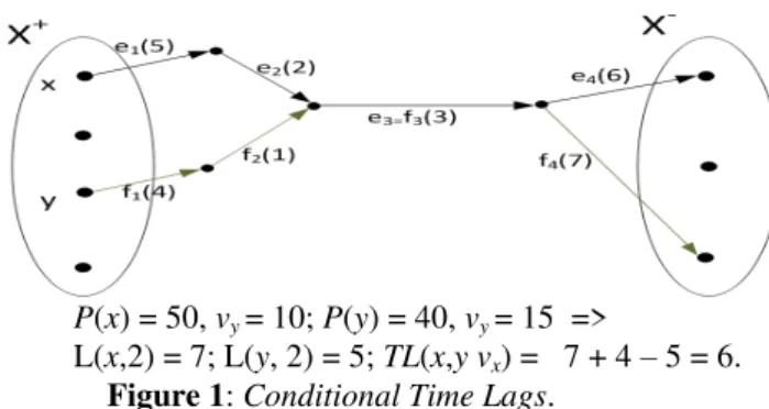
Conditional Time Lags: - If (i) = {ei1,.., e i k(i)} and (j) = {f j 1,.., f j k(j)} share arc e
= eik= fjl, and if evacuees from j come on e after
evacuees from i, then delay Tj – Ti will be no smaller
than TL-Elem(i, j, e) = L(i, k-1) – L(j, l-1) + P(i)/vi.
- Set Arc(i,j) = {e (i) (j)} and TL(i,j, vi) = Sup e Arc(i,j) (L(i, k-1) – L(j, l-1) + P(i)/vi) = Conditional
Time Lag between i and j. If Arc(i,j) ≠ Nil and evacuees of j enter after evacuees of i on the arcs of
Arc(i,j), then we must have Tj ≥ Ti + TL(i,j, vi). We
notice TL(i,j, vi) depends in a convex way on the
evacuation rate vi of i.
This notion is illustrated by following Figure 1:
P(x) = 50, vy = 10; P(y) = 40, vy = 15 =>
L(x,2) = 7; L(y, 2) = 5; TL(x,y vx) = 7 + 4 – 5 = 6.
Figure 1: Conditional Time Lags.
We derive a RCPSP (Resource Constrained Scheduling: [5,6]) reformulation of NEPP, which relies on the fact that we consider every evacuation job i N+ as a job, whose execution requires resources which are arcs e
(i), constrained by their capacities CAP(e) and whose
start-dates are constrained by conditional time lags:
NPEP-RCPSP Model :
{Preliminary : We add to the set N+ two fictitious jobs
s (source) and p (sink), in order to express the way resources are exchanged between jobs as a flow vector. Then we set, for any i N+
: TL(s,i, CAP(e)) = 0 and TL(i,p, vi) = L_TIME(i) + P(i)/vi.
Output Vectors : For any i in N+ {s,p} compute
start-date Ti and evacuation rate vi; In order to do it
we involve, for any pair (i,j) and any arc e in Arc(i,j) the part wi,j,e of access rate to e which is given by i to j
Constraints :
o For any i p, Ti + L_TIME(i) + P(i)/ vi ≤ (i) ;
(*Deadline Constraints*) (E1) o for any pair (i,j) and any e in Arc(i,j), wi,j,e ≠ 0 ->
Tj ≥ Ti + TL(i,j, vi); (*Conditional Time Lag
Constraints*) (E2) o Ts = 0 ; (E3)
o For any i in N+, N+ and any arc e in (i), (*Flow
Constraints*): j such that e Arc(x,y) wi,j,e = vi
= j such that e Arc(j,i) wj,i,e; (E4)
o For any arc e of the transit network H : (*Flow
Constraints*):CAP(e) = i such that e (i) ws,i,e
= i such that e (i) wi,p,e; (E5)
o For any i dans N+, v-Min(i) ≤ vi ≤ v-Max(i). (E6)
Maximize: i P(i).((i) – Ti – L_TIME(i) - P(i)/vi)
Explanation: (E1) tells that every evacuation job i must
be achieved before deadline (i). (E2) means that if job i provides j with some access to arc e, then the conditional
time lag inequality holds. (E4, E5) express Flow Kirshoff laws: arcs e are resources that evacuation jobs exchange between them; so job i receives vi resource (evacuation
rate) for any e (i) and no more than CAP(e) such resource may be simultaneously distributed between
evacuation jobs .
IV. ALGORITHMS
NMEP model contains both NP-Hard RCPSP and TSP problems. We have to choose between assigning high
rates vi to jobs i or let them monopolize the access to
transit arcs, or conversely restricting vi in order to make i
share its arcs. In order to do it, we implement a two-step approach: MNEP-First-Step searches a feasible schedule satisfying (E1,..,E6), while MNEP-Second-Step increases
rates vi in order to improve the weighted safety margin.
A. The Greedy-NPEP Process.
Greedy-NPEP starts from some linear ordering defined
on N+ {s,p}, and considers at any time some job i0
such that for any j prior to i0 according to , vj, Tj and
values (j,e) = access level to arc e that job j can transmit to i0 are available.Then it applies a 3 stage function
Assign(i0) which computes (see Fig. 1) vi0, Ti0 and flow
values wj,i0,e, j s.t j i0, and e Arc(j,i0), or, in case of
failure, a job j-fail i0 considered as cause of the failure.
- (1) : Assign scans path (i0), and for any e in (i0),
provides i0 with access rate to e in such a way
resulting end-date T*i0 ≤ (i0). (see Fig. 2): Assign1
For e in (i0) do
Let L-Job = {j s.t (j i0) AND (e Arc(j, i0) AND
((j, e) 0), ordered according to increasing Tj +
TL(j, i0, vj) values}; v <- 0 ; Not Stop ;
While L-Job ≠ Nil AND Not Stop do
If Tj+ TL(j, i0, vj) + L_TIME(x0) +
P(i0)/(v+(j, e)) ≤ (i0) then
Compute w such that Tj + TL(j, i0, v(j)) +
L_TIME(x0) + P(i0)/(v+w) = (i0);
Stop ; v <- v + w ; wj,i0,e<- w ;
Else v <- (j,e) + v; wj,i0,e<- (x,e) ;
If Not Stop then Fail : Choose j-Fail in L-Job Else v-aux(e) <- v ;
If Not Fail then Vi0 <- Sup e v-aux(e); e0 <- Arg Sup.
= s,…, x1, …, x2, ….x3, …., x0,…. (x0) = {e1, e2}; CAP(e1) = 20, CAP(e2) = 25; (x0); P(x0) = 50; L_TIME(x0 ) = 10; Arc(x2, x0) = {e1}; Arc(x1, x0) = {e1, e2}; Arc(x3, x0) = {e2}; TL(s, x0) = 0; TL(x1, x0) = 6; TL(x2, x0) = 3; TL(x3, x0) = 4; =>
Assign-1 -> ws,x0,e1= 2; ws,x0,e2= 3; wx1,x0,e1= 8; vx0
= 10; Success; Assign- 2 -> wx2,x0,e2= 7; Success;
Assign-3 -> wx1,x0,e1= 0; wx2,x0,e1= 8; Tx0 = 21.
Figure 2: Assign Process.
- (2) : Assign1 computes vi0 and, for any e ≠ e0 in (i0)
a value v-aux(e) which may be less than vi0; So
Assign2 increases the wj,i0,e for e e0 in order to
make job i0 run at the same rate for all arcs e of (i0). This part of the Assign process may induce a
failure which Assign2 assign to some job j-Fail.
- (3): Assign3 makes decrease the number of arcs
provided with non null wj,i0,e values by shifting
values wj,i0,e which involve, for a given j, only one
arc e, to another job j’ such that e Arc(j’, i0),
wj’,i0,e ≠ 0 and (j’, e) ≥ wj,i0,e + wj’,i0,e.
Then Greedy-NPEP comes as follows:
Greedy-RCPSP-TL() :
Ts <- 0 ; For any arc e do (s, e) <- CAP(e); Not Stop;
While (Not Stop) and no fully scanned do Apply Assign to current i0 and partial schedule;
If Success(Assign) then
For e in (i0) and j s.t (j i0) (e Arc(j,i0))
do (i0, e) <- vi0; (j,e) <- (j,e) - wj,i0,e;
Else Stop ; Return the pair (j-Fail, i0).
B. NPEP-First-Step
Greedy-NPEP may fail even in the case when a solution (T, v, w) exists. It raises the question of the way we deal with linear ordering .
Initialization of : For any i, we set SME(i) = (i) –
L_TIME(i) – 2.P(i)/(v-max(i) + v-min(i)), and compute by randomly sorting N+
in such a way that if P(i) < P(j) and SME(i) < SME(j), then i j.
Makingevolve. In case of failure, Greedy-NPEP
returns a pair (j-Fail, i0), and this pair is inserted into
a Tabu like set FORBID whose meaning is: If (j, i) is FORBID, then we should have (i j).
So, global process NPEP-First-Step comes as follows:
Procedure NPEP-First-Step(Max-Iter: Threshold)
Initialize as described above ; FORBID <- Nil ;
Iter <- 0 ; Not Stop ; Success <- 0 ;
While (Iter ≤ Iter-Max) AND (Not Success) do Generate consistent with FORBID and Apply
Greedy-NPEP; If Failure then Search a failure
responsible (j-Fail, i0) pair and put into FORBID.
C. NPEP-Second-Step
In case NPEP-First-Step yields a feasible solution (T, v,
w) NPEP-Second-Step improves it, by acting on rates vi
in such a way time lags L_TIME(i) + P(i)/vi decrease in
an ad hoc way. Let us denote by U-Active, the set of pairs (i,j) which are allowed to support non null wi,j,e flow
values. We notice that if U-Active is fixed, then resulting restriction of NPEP is a convex optimization problem defined on the (v,w) polyhedron defined by (E4, E5, E6). So we fix U-Active according to the end of
NPEP-First-Step, and deal with induced convex program:
- We derive from current v, w, values T*i, related
critical paths, and values = i), i N+ ≥ 0, such that i P(i). T*i = i (i)/vi + Constant: Vector Grad
= (Gradi = - (i)/v 2
i, i N +
) is a sub-gradient vector; - Then we modify v and w according to (I1): v <- v +
V ; w <- w + W, with V and W s.t V.Grad < 0 and v +
V and w + W comply with (E4, E5, E6) and computed by solving Project-Grad following linear program:
Project-Grad(U-Active, v, w, , Grad) LP :
{Compute V= (Vi, i N +
), and W = (Wi,j,e, (i, j)
U-Active, e Arc(i,j)) such that;
o (i,j, e), wi,j,e + Wi,j,e ≥ 0 ;
o i s,p, e (i), j Wi,j,e = j Wj,I,e = Vi ;
o e, j Ws, j, e = j Wj,p, e = 0 ;
o i ≠ s,p, v-Min(i) ≤ vi + Vi ≤ v-Max(i) ;
o 2. ≥ i ≠ s,p Vi.Grad(i) ≥ }
Then NPEP-Second-Step comes as follows:
Procedure NPEP-Second-Step:
Let (T, v, w) be the feasible solution computed by
NPEP-First-Step and T* related end-date vector; Derive U-Active; Not Stop ; Val <- i P(i). T*i;
While Not Stop do
Compute and coefficients (i), i N; Solve Project-Grad(U-Active, v, w, , Grad); If no solution then Stop Else
Apply (I1), update Ti, T*i and related
critical paths; If Val-Aux = i P(i).Ti; If
Val-Aux≥ Val then Stop.
V. NUMERICAL EXPERIMENTS.
Purpose: Algorithms were implemented on AMD
Opteron 2.1GHz. Our goal was to evaluate the ability of
NPEP-First-Step to deal with tight deadlines and the ability of NPEP-Second-Step to improve this solution.
Instances/outputs: An instance is a path collection {(i),
i N+}, given together with values P(i), (i) and
TIME(eik). It is summarized by a 3-uple: (n, m, ), where
n = Car(N+), m = number of arc e, and is as above. We both created our own instances and used an instance generator of [1].In order to get benchmarks, we generated
ad hoc schedules (T, v) and derived deadlines (i) which
made us be provided with almost optimal solutions.
Outputs: For every 10 instance package, we compute:
- The number Trial of iterations on necessary to get a feasible solution through NPEP-First-Step; - The improvement margin (%) IMPROVE induced
by NPEP-Second-Step;
- The gap between NPEP .and optimal value VAL
Table below provides results for [1,2]. Inst. 1: n = 20, m = 10 Trial IMPROVE (%) GAP (%) CPU-NPEP = 1.2 22.30 13.8 4.7 40.4 = 1.5 2.50 29.5 13.0 12.3 = 1.7 1.39 40.8 17.7 8.1 = 2.0 1.08 61.7 19.3 5.2 Inst. 1: n = 30, m = 15 = 1.2 40.6 14.6 5.6 70.5 = 1.5 6.60 30.2 14.5 19.5 = 1.7 2.05 42.3 19.1 12.0 = 2.0 1.19 65.5 22.5 7.9
Comment: Tighting deadlines (i) improve solutions.
VI. CONCLUSION
We described here a two-step RCPSP oriented algorithm for the NPEP Problem. Remains now to deal with the design of an exact method for small instances and with an integrated computation of routes (i).
REFERENCES
[1] C.Artigues, E.Hebrard, Y.Pencolé, A.Schutt, P.Stuckey: A study of evacuation planning for wildfires; 17 th Int. Workshop on
Constraint Modelling/Reformulation, Lille, France, (2018).
[2] V.Bayram : Optimization models for large scale network evacuation planning and management : a review ; Surveys in O.R
and Management, (2016), DOI : 10.1016/j.sorms.2016.11.001.
[3] C.Even, V.Pillac, P.Van Hentenryk: Convergent plans for large scale evacuation; In Proc. 29 th AAAI Conf. On Artificial
Intelligence, Austin, Texas, p 1121-1127, (2015).
[4] Geo-Safe-; MSCA-RISE 2015 European Project –id 691161. http://fseg.gre.ac.uk/fire/geo-safe.html. Accessed Jue 12, (2018).
[5] M.J. Orji, S. Wei. Project Scheduling Under Resource Constraints: A Recent Survey. Inter. Journal of Engineering
Research & Technology (IJERT) Vol. 2 Issue 2, (2013)
[6] A.Quilliot, H.Toussaint: Flow Polyedra and RCPSP,
RAIRO-RO, 46-04, p 379-409, (2012)