EUROPEAN ORGANISATION FOR NUCLEAR RESEARCH (CERN)
Eur. Phys. J. C 80 (2020) 1080
DOI:10.1140/epjc/s10052-020-08469-8
CERN-EP-2020-074 18th December 2020
Search for top squarks in events with a Higgs or 𝒁
boson using 139 fb
√
−1
of 𝒑 𝒑 collision data at
𝒔 = 13 TeV with the ATLAS detector
The ATLAS Collaboration
This paper presents a search for direct top squark pair production in events with missing transverse momentum plus either a pair of jets consistent with Standard Model Higgs boson decay into 𝑏-quarks or a same-flavour opposite-sign dilepton pair with an invariant mass consistent with a 𝑍 boson. The analysis is performed using the proton–proton collision data at √
𝑠 = 13 TeV collected with the ATLAS detector during the LHC Run-2, corresponding to an integrated luminosity of 139 fb−1. No excess is observed in the data above the Standard Model predictions. The results are interpreted in simplified models featuring direct production of pairs of either the lighter top squark (˜𝑡1) or the heavier top squark (˜𝑡2), excluding at 95%
confidence level ˜𝑡1and ˜𝑡2masses up to about 1220 and 875 GeV, respectively.
© 2020 CERN for the benefit of the ATLAS Collaboration.
Reproduction of this article or parts of it is allowed as specified in the CC-BY-4.0 license.
1 Introduction
Supersymmetry (SUSY) [1–6] is one of the most studied frameworks to extend the Standard Model (SM) beyond the electroweak scale. It predicts new bosonic (fermionic) partners for the known fermions (bosons). Assuming 𝑅-parity conservation [7], SUSY particles are produced in pairs and the lightest supersymmetric particle (LSP) is stable, providing a possible dark-matter candidate. The SUSY partners of the Higgs bosons and electroweak gauge bosons mix to form the mass eigenstates known as charginos ( ˜𝜒±
𝑘, 𝑘 = 1, 2)
and neutralinos ( ˜𝜒0
𝑚, 𝑚 = 1, 2, 3, 4), where the increasing index denotes increasing mass. The scalar
partners of right-handed and left-handed quarks, ˜𝑞
Rand ˜𝑞L squarks, mix to form two mass eigenstates, ˜𝑞1
and ˜𝑞
2, with ˜𝑞1defined to be the lighter of the two. To address the SM hierarchy problem [8–11], TeV-scale
masses are favoured [12,13] for the supersymmetric partners of the gluons, and the top squarks [14,15]. Top squark production with SM Higgs (ℎ) or 𝑍 bosons in the decay chain can appear either in production of the lighter top squark mass eigenstate (˜𝑡1) decaying via ˜𝑡1→ 𝑡 ˜𝜒
0 2 with ˜ 𝜒0 2 → ℎ/𝑍 ˜ 𝜒0 1, or in production
of the heavier top squark mass eigenstate (˜𝑡2) decaying via ˜𝑡2 → 𝑍 ˜𝑡1with ˜𝑡1 → 𝑡 (∗)𝜒˜0
1, as illustrated in
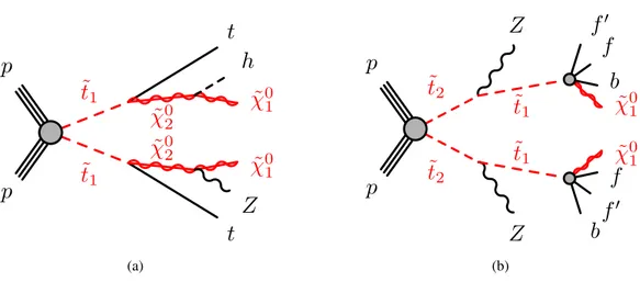
Figure1. Unlike other top squark models, these signals can be efficiently distinguished from the SM top quark pair production (𝑡 ¯𝑡) background by requiring either a same-flavour opposite-sign (SF-OS) lepton pair originating from the 𝑍 → ℓ+ℓ−(ℓ ≡ 𝑒, 𝜇) decay or a pair of 𝑏-tagged jets originating from the ℎ → 𝑏 ¯𝑏 decay, plus the presence of an additional lepton produced in the decay of the top quarks in the event. Simplified models [16–18] are used for the analysis optimisation and interpretation of the results. In these models, direct top squark pair production is considered and all SUSY particles are decoupled except for the top squarks and the neutralinos involved in their decay. In all cases the ˜𝜒01is assumed to be the LSP.
Simplified models featuring direct ˜𝑡1production with ˜𝑡1 → 𝑡 ˜𝜒 0
2 and decays via either Higgs ( ˜
𝜒0 2 → ℎ ˜ 𝜒0 1) or 𝑍 ( ˜𝜒20→ 𝑍 ˜ 𝜒0
1) bosons with different branching ratio values are considered. In these models, the ˜
𝜒0
1 is
assumed to be very light and the ˜𝜒20− ˜
𝜒0
1 mass difference to be large enough to allow on-shell Higgs or 𝑍
boson decays.
Additional simplified models featuring direct ˜𝑡2production with ˜𝑡2→ 𝑍 ˜𝑡1decays and ˜𝑡1 → 𝑡 (∗)𝜒˜0
1 are also
considered. The mass difference between the ˜𝑡1and ˜
𝜒0
1 is set to be smaller than the 𝑊 boson mass, and
the four-body decay ˜𝑡1 → 𝑏 𝑓 𝑓 0
˜ 𝜒0
1 is assumed to occur, where 𝑓 and 𝑓 0
are two fermions from the 𝑊∗ decay, such as ˜𝑡1 → 𝑏ℓ𝜈 ˜𝜒
0
1. Direct production of ˜𝑡1pairs is not considered in the ˜𝑡2production simplified
models. The ˜𝑡1pair production contribution to the selections presented in this paper has been found to be
negligible.
This paper presents the results of a search for top squarks in final states with Higgs or 𝑍 bosons at√ 𝑠= 13 TeV using the complete data sample collected with the ATLAS detector [19] in proton–proton (𝑝 𝑝) collisions during Run-2 of the LHC (2015–2018), corresponding to 139 fb−1. Searches for top squark production in events involving Higgs or 𝑍 bosons have been performed previously by both ATLAS [20,
˜
t
1˜
t
1˜
χ
02˜
χ
02p
p
t
˜
χ
01h
t
˜
χ
01Z
(a)˜
t
2˜
t
2˜
t
1˜
t
1p
p
Z
˜
χ
01b
f
f
0Z
˜
χ
01b
f
0f
(b)Figure 1: Diagrams for the top squark pair production processes considered in this analysis: (a) ˜𝑡1 → 𝑡 ˜𝜒 0 2 with ˜ 𝜒0 2 → ℎ/𝑍 ˜𝜒 0
1 decays (showing for illustration the case where the two ˜𝜒 0
2 decay differently, although events with the
same ˜𝜒0
2 decays are also considered in the analysis), and (b) ˜𝑡2→ 𝑍 ˜𝑡1with ˜𝑡1 → 𝑏 𝑓 𝑓 0
˜ 𝜒0
1 decays.
2 ATLAS detector
The ATLAS detector [19,24] at the LHC is a multipurpose particle detector with a forward–backward symmetric cylindrical geometry and a near 4𝜋 coverage in solid angle.1 It consists of an inner tracking detector (ID) surrounded by a thin superconducting solenoid providing a 2 T axial magnetic field, electromagnetic (EM) and hadron calorimeters, and a muon spectrometer (MS). The inner tracking detector covers the pseudorapidity range |𝜂| < 2.5. It consists of silicon pixel, silicon microstrip, and transition radiation tracking detectors. Lead/liquid-argon (LAr) sampling calorimeters provide EM energy measurements with high granularity. A steel/scintillator-tile hadron calorimeter covers the central pseudorapidity range |𝜂| < 1.7. The endcap and forward regions are instrumented with LAr calorimeters for both the EM and hadronic energy measurements up to |𝜂| = 4.9. The muon spectrometer surrounds the calorimeters and is based on three large air-core toroidal superconducting magnets with eight coils each. The field integral of the toroids ranges between 2 and 6 T m across most of the detector. The muon spectrometer includes a system of precision tracking chambers and fast detectors for triggering. A two-level trigger system is used to select events [25]. The first-level trigger is implemented in hardware and uses a subset of the detector information to reduce the accepted rate to at most 100 kHz. This is followed by a software-based trigger that reduces the accepted event rate to 1 kHz on average depending on the data-taking conditions.
3 Data set and simulated event samples
The data were collected by the ATLAS detector during the LHC Run-2 (2015–2018) with a peak instantaneous luminosity of L = 2.1 × 1034cm−2s−1, resulting in a mean number of 𝑝 𝑝 interactions per
1ATLAS uses a right-handed coordinate system with its origin at the nominal interaction point (IP) in the centre of the detector
and the 𝑧-axis along the beam pipe. The 𝑥-axis points from the IP to the centre of the LHC ring, and the 𝑦-axis points upwards. Cylindrical coordinates (𝑟, 𝜙) are used in the transverse plane, 𝜙 being the azimuthal angle around the 𝑧-axis. The pseudorapidity
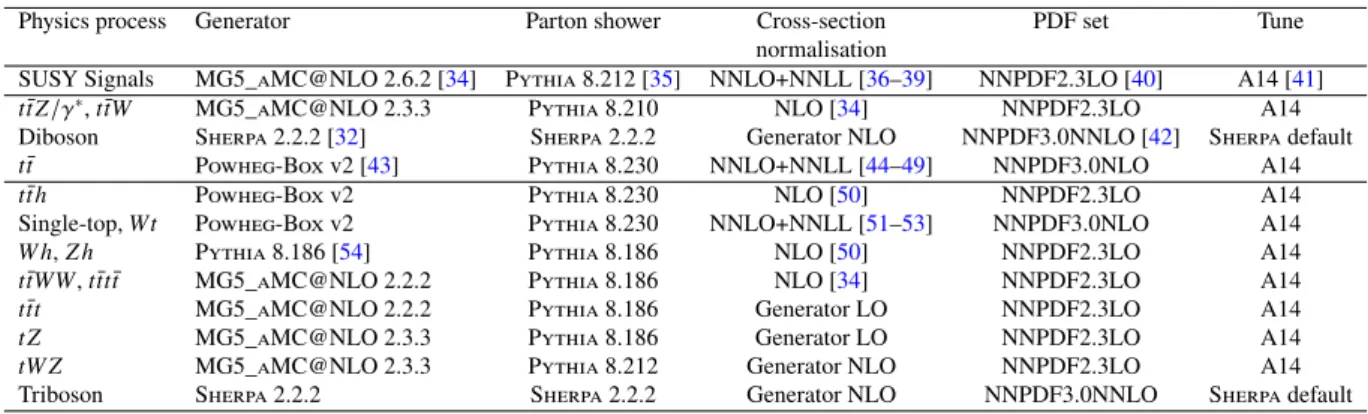
Table 1: Simulated signal and background event samples: the corresponding event generator used for the hard-scatter process, the generator used to model the parton showering, the source of the cross-section used for normalisation, the PDF set and the underlying-event tune are shown.
Physics process Generator Parton shower Cross-section PDF set Tune
normalisation
SUSY Signals MG5_aMC@NLO 2.6.2 [34] Pythia 8.212 [35] NNLO+NNLL [36–39] NNPDF2.3LO [40] A14 [41]
𝑡¯𝑡𝑍 /𝛾∗, 𝑡 ¯𝑡𝑊 MG5_aMC@NLO 2.3.3 Pythia 8.210 NLO [34] NNPDF2.3LO A14
Diboson Sherpa 2.2.2 [32] Sherpa 2.2.2 Generator NLO NNPDF3.0NNLO [42] Sherpa default
𝑡¯𝑡 Powheg-Box v2 [43] Pythia 8.230 NNLO+NNLL [44–49] NNPDF3.0NLO A14
𝑡¯𝑡ℎ Powheg-Box v2 Pythia 8.230 NLO [50] NNPDF2.3LO A14
Single-top, 𝑊 𝑡 Powheg-Box v2 Pythia 8.230 NNLO+NNLL [51–53] NNPDF3.0NLO A14
𝑊 ℎ, 𝑍 ℎ Pythia 8.186 [54] Pythia 8.186 NLO [50] NNPDF2.3LO A14
𝑡¯𝑡𝑊𝑊 , 𝑡 ¯𝑡𝑡 ¯𝑡 MG5_aMC@NLO 2.2.2 Pythia 8.186 NLO [34] NNPDF2.3LO A14
𝑡¯𝑡𝑡 MG5_aMC@NLO 2.2.2 Pythia 8.186 Generator LO NNPDF2.3LO A14
𝑡 𝑍 MG5_aMC@NLO 2.3.3 Pythia 8.186 Generator LO NNPDF2.3LO A14
𝑡𝑊 𝑍 MG5_aMC@NLO 2.3.3 Pythia 8.212 Generator NLO NNPDF2.3LO A14
Triboson Sherpa 2.2.2 Sherpa 2.2.2 Generator NLO NNPDF3.0NNLO Sherpa default
bunch crossing of h𝜇i = 34. Data quality requirements are applied to ensure that all subdetectors were operating normally, and that the LHC beams were in stable-collision mode. The integrated luminosity of the resulting data sample is 139 fb−1. The uncertainty in the combined 2015–2018 integrated luminosity is 1.7%. It is derived from the calibration of the luminosity scale using 𝑥–𝑦 beam-separation scans, following a methodology similar to that detailed in Ref. [26], and using the LUCID-2 detector for the baseline luminosity measurements [27].
Monte Carlo (MC) simulated event samples are used to aid the estimation of the background from SM processes and to model the SUSY signal. The choices of MC event generator, parton shower and hadronisation, the cross-section normalisation, the parton distribution function (PDF) set and the set of tuned parameters (tune) for the underlying event of these samples are summarised in Table1. More details of the event generator configurations can be found in Refs. [28–31]. Cross-sections calculated at next-to-next-to-leading order (NNLO) in quantum chromodynamics (QCD) including resummation of next-to-next-to-leading logarithmic (NNLL) soft-gluon terms were used for top quark production processes. For production of top quark pairs in association with vector or Higgs bosons, cross-sections calculated at next-to-leading order (NLO) were used, and the event generator NLO cross-sections from Sherpa [32] were used when normalising the multi-boson backgrounds. In all MC samples, except those produced by Sherpa, the EvtGen v1.2.0 program [33] was used to model the properties of the bottom and charm hadron decays.
SUSY signal samples were generated with MG5_aMC@NLO 2.6.2 [34] interfaced to Pythia 8.212 [35] for the parton showering (PS) and hadronisation. The matrix element (ME) calculation was performed at tree level and includes the emission of up to two additional partons for all signal samples. MadSpin [55] was used to model the ˜𝑡1 → 𝑏 𝑓 𝑓
0𝜒˜0
1 decays. MadSpin emulates kinematic distributions to a good
approximation without calculating the full ME. The PDF set used for the generation of the signal samples was NNPDF2.3LO [40] with the A14 [41] set of tuned underlying-event and shower parameters (UE tune). The ME–PS matching was performed with the CKKW-L prescription [56], with a matching scale set to one quarter of the top squark mass. All signal cross-sections were calculated to approximate NNLO in the strong coupling constant, adding the resummation of soft gluon emission at NNLL accuracy (approximate NNLO+NNLL) [36–39]. The nominal cross-section and its uncertainty were derived using
To simulate the effects of additional 𝑝 𝑝 collisions in the same and nearby bunch crossings (pile-up), additional interactions were generated using the soft QCD processes provided by Pythia 8.186 with the A3 tune [58] and the MSTW2008LO PDF set [59], and overlaid onto each simulated hard-scatter event. The MC samples were reweighted so that the pile-up distribution matches the one observed in the data. The MC samples were processed through an ATLAS detector simulation [60] based on Geant 4 [61] or, in the case of 𝑡 ¯𝑡𝑡 and the SUSY signal samples, a fast simulation using a parameterisation of the calorimeter response and Geant 4 for the other parts of the detector. All MC samples were reconstructed in the same manner as the data.
4 Event selection
Candidate events are required to have a reconstructed vertex [62] with at least two associated tracks with transverse momentum (𝑝T) larger than 500 MeV that are consistent with originating from the beam collision
region in the 𝑥–𝑦 plane. The primary vertex in the event is the vertex with the highest sum of squared transverse momenta of associated tracks.
Two categories of leptons (electrons and muons) are defined: ‘candidate’ and ‘signal’ (the latter being a subset of the ‘candidate’ leptons satisfying tighter selection criteria). Electron candidates are reconstructed from isolated electromagnetic calorimeter energy deposits matched to ID tracks and are required to have |𝜂| < 2.47, a transverse momentum 𝑝T > 4.5 GeV, and to satisfy the ‘LooseAndBLayer’ requirement
defined in Ref. [63], which is based on a likelihood using measurements of shower shapes in the calorimeter and track properties in the ID as input variables.
Muon candidates are reconstructed in the region |𝜂| < 2.4 from MS tracks matching ID tracks. Candidate muons are required to have 𝑝T > 4 GeV and satisfy the ‘medium’ identification requirements defined in
Ref. [64], based on the number of hits in the different ID and MS subsystems, and on the ratio of the charge and momentum (𝑞/𝑝) measured in the ID and MS divided by the sum in quadrature of their corresponding uncertainties.
The tracks associated with the lepton candidates are required to have a significance of the transverse impact parameter relative to the reconstructed primary vertex, 𝑑0, of |𝑑0|/𝜎 (𝑑0) < 5 for electrons and
|𝑑0|/𝜎 (𝑑0) < 3 for muons, and a longitudinal impact parameter relative to the reconstructed primary vertex, 𝑧0, satisfying |𝑧0sin 𝜃 | < 0.5 mm.
Jets are reconstructed from three-dimensional energy clusters in the calorimeter [65] using the anti-𝑘𝑡 jet
clustering algorithm [66] with a radius parameter 𝑅 = 0.4. Only jet candidates with 𝑝T > 20 GeV and
|𝜂| < 2.8 are considered. Jets are calibrated using MC simulation with corrections obtained from in situ techniques [67]. To reduce the effects of pile-up, jets with 𝑝T <120 GeV and |𝜂| < 2.5 are required to
have a significant fraction of their associated tracks compatible with originating from the primary vertex, as defined by the jet vertex tagger [68]. This requirement reduces the fraction of jets from pile-up to 1%, with an efficiency for hard-scatter jets of about 90%. Events are discarded if they contain any jet with 𝑝T > 20 GeV not satisfying basic quality selection criteria designed to reject detector noise and
non-collision backgrounds [69].
Identification of jets containing 𝑏-hadrons (𝑏-tagging) is performed with a multivariate discriminant that makes use of track impact parameters and reconstructed secondary vertices [70,71]. Jets are considered as 𝑏-tagged if they fulfil a requirement corresponding to a 77% average efficiency obtained for jets containing 𝑏-hadrons in simulated 𝑡 ¯𝑡 events. The rejection factors for light-quark and gluon jets, jets containing
𝑐-hadrons and jets containing hadronically decaying 𝜏-leptons in simulated 𝑡 ¯𝑡 events are approximately 113, 16 and 4, respectively.
Jet candidates with 𝑝T < 200 GeV within an angular distance Δ𝑅 =
√︁
(Δ𝑦)2+ (Δ𝜙)2 = 0.2 of an electron
candidate are discarded, unless the jet has a value of the 𝑏-tagging discriminant larger than the value corresponding to approximately 85% 𝑏-tagging efficiency, in which case the lepton is discarded since it is likely to have originated from a semileptonic 𝑏-hadron decay. The same procedure is applied to jets within Δ𝑅 = 0.2 of a muon candidate irrespective of the jet 𝑝T. Any remaining electron candidate within
Δ𝑅 = 0.4 of a non-pile-up jet, and any muon candidate within Δ𝑅 = min{0.4, 0.04 + 𝑝T( 𝜇)/10 GeV} of a
non-pile-up jet is discarded. In the latter case, if the jet has fewer than three associated tracks, the muon is retained and the jet is discarded instead to avoid inefficiencies for high-energy muons undergoing significant energy loss in the calorimeter. Finally, any electron candidate sharing an ID track with a remaining muon candidate is also removed.
Tighter requirements on the lepton candidates are imposed, which are then referred to as ‘signal’ electrons or muons. Signal electrons must satisfy the ‘Medium’ identification requirement as defined in Ref. [63] and signal muons must have 𝑝T >5 GeV. Isolation requirements are applied to both the signal electrons and
muons. The scalar sum of the 𝑝Tof tracks within a variable-size cone around the lepton, excluding its own
track, must be less than 6% of the lepton 𝑝T; these tracks are required to be associated with the primary
vertex to limit sensitivity to pile-up. The size of the track isolation cone for electrons (muons) is given by the smaller of Δ𝑅 = 10 GeV/𝑝Tand Δ𝑅 = 0.2 (0.3). In addition, in the case of electrons the energy of
calorimeter energy clusters in a cone of Δ𝑅𝜂 =
√︁
(Δ𝜂)2+ (Δ𝜙)2 = 0.2 around the electron (excluding the
deposition from the electron itself) must be less than 6% of the electron 𝑝T.
Simulated events are corrected for differences between data and MC simulation in jet vertex tagger and 𝑏-tagging efficiencies as well as 𝑏-tagging mis-tag rates [68,71–73]. Corrections are also applied to account for minor differences between data and MC simulation in the signal-lepton trigger, reconstruction, identification and isolation efficiencies.
The missing transverse momentum vector, whose magnitude is denoted by 𝐸Tmiss, is defined as the negative vector sum of the transverse momenta of all identified electrons, muons and jets, plus an additional soft term. The soft term is constructed from all tracks that originate from the primary vertex but are not associated with any identified lepton or jet. In this way, the 𝐸Tmissis adjusted for the best calibration of leptons and jets, while contributions from pile-up interactions are suppressed through the soft term [74,
75].
The events are classified into two exclusive categories: at least three leptons (referred to as 3ℓ selection, aimed at top squark decays involving 𝑍 bosons), or exactly one lepton (referred to as 1ℓ selection, aimed at top squark decays involving Higgs bosons). The selection requirements for each of these categories are described below.
4.1 3ℓ selection
In this selection, events are accepted if they satisfy a trigger requiring either two electrons, two muons or an electron and a muon. The requirements imposed offline on the 𝑝T, identification and isolation of
the leptons involved in the trigger decision are tighter than those applied online, so as to be on the trigger efficiency plateau [25]. The presence of at least three signal leptons (electrons or muons, referred to
with the 𝑍 boson mass (|𝑚ℓ ℓ− 𝑚𝑍| < 15 GeV, with 𝑚𝑍 = 91.2 GeV) is required. In addition, the leading
(highest 𝑝T) lepton is required to have 𝑝T > 40 GeV and the subleading to have 𝑝T > 20 GeV. The SF-OS
requirements are not applied for the validation of the background induced by fake and non-prompt leptons in Section5.1.
Four overlapping signal regions (SRs) are optimised for the best discovery sensitivity, two for each of the simplified models described in Section1. The requirements in each SR are summarised in Table2. Signal region SR1A𝑍 is optimised for large ˜𝜒20− ˜
𝜒0
1 mass splittings in the ˜𝑡1 → 𝑡 ˜
𝜒0 2 with ˜ 𝜒0 2 → ℎ/𝑍 ˜ 𝜒0 1
model. It includes requirements on 𝑚3ℓT2, a variation of the stransverse mass 𝑚T2which is used to bind the
masses of a pair of particles that are presumed to have each decayed semi-invisibly into one visible and one invisible particle [76,77]. In the case of 𝑚3ℓT2, the two visible legs of the two semi-invisible decays are set to be the third leading lepton and the system of the SF-OS lepton pair with an invariant mass closest to 𝑚𝑍. Models with small mass differences between the ˜𝜒
0
2and the ˜𝜒 0
1are targeted with SR 𝑍
1B, which instead
imposes requirements on the transverse momentum of the SF-OS lepton pair (𝑝ℓ ℓT ). Two SRs are optimised for the ˜𝑡2→ 𝑍 ˜𝑡1with ˜𝑡1 → 𝑏 𝑓 𝑓
0𝜒˜0
1model, SR 𝑍
2Aand SR 𝑍
2B, targeting small and
large mass splittings between the ˜𝑡2and the ˜𝜒 0
1, respectively. Due to the overall soft kinematics of the
particles in compressed ˜𝑡2signals, SR 𝑍
2Afeatures upper bounds on the 𝑝Tof the third leading lepton and
on 𝑝ℓ ℓT , as well as no requirement on the number of 𝑏-tagged jets since they are likely to be soft in this scenario. SR2B𝑍 also includes an upper bound on the third leading lepton 𝑝Tbut requires the presence of
𝑏-tagged jets and large 𝐸miss
T and 𝑝
ℓ ℓ T .
The requirement on the number of signal leptons makes the SR1A𝑍 and SR𝑍1B selections insensitive to potential contributions from alternative ˜𝑡1decays with each ˜𝑡1 → 𝑡 ˜𝜒
0
1. The acceptance for mixed decay
scenarios, with ˜𝑡1˜𝑡1 → 𝑡 ˜𝜒 0 1𝑡𝜒˜
0
2 was found to depend linearly on the branching fraction of ˜𝑡1to 𝑡 ˜𝜒 0 2. The
signal lepton multiplicity requirement depletes the contribution from the direct production of ˜𝑡1pairs to
SR𝑍2Aand SR𝑍2B.
4.2 1ℓ selection
Events in this selection are accepted if they satisfy a combination of single-lepton and 𝐸Tmiss trigger requirements, the latter being used only for events with 𝐸Tmiss> 230 GeV and lepton 𝑝
T <30 GeV. The
offline requirements on the 𝐸Tmiss, 𝑝T, identification and isolation of the lepton are tighter than those applied
online, so as to be on the trigger efficiency plateau [25]. The presence of exactly one signal lepton (electron or muon) is required.
The identification of Higgs boson candidates decaying into 𝑏-quarks is performed using a neural network that uses as input the four-momentum and 𝑏-tagging information of pairs of jets. The scaled jet 𝑝T/𝑚𝑗 𝑗
observable is used to prevent the dijet invariant mass being used as the primary discriminating variable. The network is trained with the PyTorch package [78] using as signal dijet pairs originating from Higgs boson decays in the simulated 𝑡 ¯𝑡𝐻 process, and as background dijet pairs in 𝑡 ¯𝑡 and 𝑡 ¯𝑡𝐻 not originating from Higgs boson decays. A jet pair is tagged as a Higgs boson candidate if the corresponding neural network score is above a threshold optimised to target models predicting sizeable branching fractions of ˜𝜒20
into Higgs bosons. The efficiency to correctly identify jet pairs originating from Higgs boson decays in signal events is 50%–54% depending on the ˜𝑡1mass, as evaluated on a simulated event sample selected by
Table 2: Definition of the signal regions used in the 3ℓ selection (see text for further description).
Requirement / Region SR𝑍1A SR𝑍1B SR2A𝑍 SR𝑍2B
Number of signal leptons ≥ 3
Number of SF-OS pairs ≥ 1
Leading lepton 𝑝T[GeV] >40
Subleading lepton 𝑝T [GeV] >20
|𝑚SF-OS
ℓ ℓ − 𝑚𝑍| [GeV]
<15
Third leading lepton 𝑝T[GeV] > 20 >20 <20 <60
𝑛
jets(𝑝T >30 GeV) ≥ 4 ≥ 5 ≥ 3 ≥ 3
𝑛𝑏
-tagged jets(𝑝T >30 GeV) ≥ 1 ≥ 1 – ≥ 1
Leading jet 𝑝T[GeV] – – >150 –
Leading 𝑏-tagged jet 𝑝T[GeV] – > 100 – –
𝐸miss T [GeV] > 250 > 150 >200 >350 𝑝ℓ ℓ T [GeV] – > 150 <50 >150 𝑚3ℓ T2[GeV] > 100 – – –
requiring one signal lepton and at least two 𝑏-tagged jets. Using the same selection, the probability of tagging a jet pair in 𝑡 ¯𝑡 events is approximately 0.05%.
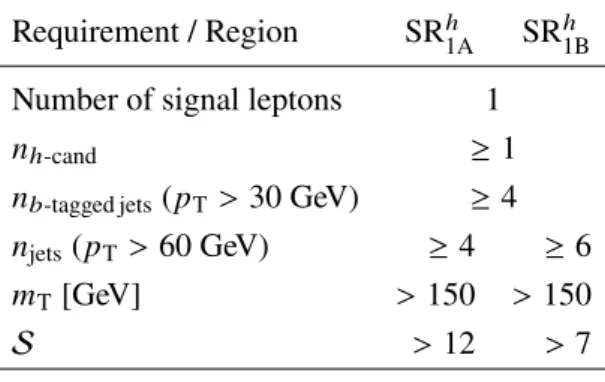
Two overlapping SRs are optimised for the best discovery sensitivity in the ˜𝑡1 → 𝑡 ˜𝜒 0
2 simplified model
discussed in Section1, and their requirements are summarised in Table3. Both require the presence of at least four 𝑏-tagged jets and at least one Higgs boson candidate (𝑛ℎ-cand). The SRs include requirements on the
transverse mass 𝑚T(computed as 𝑚T =
√︃
2𝑝ℓT𝐸miss
T (1 − cos Δ𝜙) where Δ𝜙 is the azimuthal angle between
the missing transverse momentum vector and the lepton), and on the object-based 𝐸Tmiss-significance [79] (S), which is used to discriminate events where the 𝐸Tmissis due to invisible particles in the final state from events where the 𝐸Tmissis due to poorly measured particles and jets. The requirements on 𝑛𝑏-tagged jetsand
𝑛ℎ
-candreduce the potential contributions from alternative ˜𝑡1 decays with each ˜𝑡1 → 𝑡 ˜
𝜒0
1 to a negligible
level. Analogously to the 3ℓ selection, the acceptance for mixed decay scenarios with ˜𝑡1˜𝑡1→ 𝑡 ˜
𝜒0
1𝑡˜
𝜒0
2 has
been found to depend linearly on the branching fraction of ˜𝑡1to 𝑡 ˜
𝜒0
2.
Signal region SRℎ1Ais optimised for small ˜𝜒0
2− ˜𝜒 0
1 mass splittings, while large ˜𝜒 0 2− ˜𝜒
0
1 mass splittings are
Table 3: Definition of the signal regions used in the 1ℓ selection (see text for further description).
Requirement / Region SRℎ1A SR1Bℎ
Number of signal leptons 1
𝑛ℎ
-cand ≥ 1
𝑛𝑏-tagged jets(𝑝T > 30 GeV) ≥ 4
𝑛 jets(𝑝T > 60 GeV) ≥ 4 ≥ 6 𝑚 T[GeV] >150 > 150 S > 12 >7
5 Background estimation
The dominant SM background contribution to the 3ℓ SRs is expected to originate from 𝑡 ¯𝑡𝑍 production, with minor contributions from multi-boson production (mainly 𝑊 𝑍 ) and backgrounds containing hadrons misidentified as leptons (hereafter referred to as ‘fake’ leptons) or non-prompt leptons from decays of hadrons (mainly in 𝑡 ¯𝑡 events). The main background affecting the 1ℓ SRs is expected to originate from 𝑡 ¯𝑡 production in association with heavy-flavour quarks.
The background from fake/non-prompt (FNP) leptons is estimated in a data-driven way, while the normalisation of the main backgrounds (𝑡 ¯𝑡𝑍 and multi-boson in the 3ℓ selection; 𝑡 ¯𝑡 in the 1ℓ selection) is obtained by fitting the yield from MC simulation to the observed data in dedicated control regions (CRs) enhanced in a particular background component, and then extrapolating this yield to the SRs. Backgrounds from other sources, which provide a subdominant contribution to the SRs, are determined from MC simulation only.
The expected SM background is determined separately in each SR from a profile likelihood fit [80] implemented in the HistFitter framework [81]. The fit uses as a constraint the observed event yield in the fitted regions to adjust the normalisation of the main backgrounds. The quality of the resulting background model is judged by performing a ‘background-only’ fit to data using exclusively the event yield in the CRs to adjust the normalisation of the backgrounds. The agreement of the resulting background model is compared with the data yields in dedicated validation regions (VRs). Systematic uncertainties related to the MC modelling affect the expected yields in the SRs and CRs, and are taken into account to determine the uncertainty in the background prediction. Each source of uncertainty is described by a single nuisance parameter, and correlations between background processes and selections are taken into account. The VRs, used to assess the quality of the background model, are not used to constrain the nuisance parameters in the fit. The fit does not significantly affect either the uncertainty or the central value of these nuisance parameters. The systematic uncertainties considered in the fit are described in Section6.
5.1 Fake/non-prompt lepton background
A method similar to that described in Refs. [82,83] is used for the estimation of the FNP lepton background. Two types of lepton identification criteria are defined for this evaluation: ‘tight’ and ‘loose’, corresponding
to the signal and candidate electrons and muons described in Section4. With the number of observed events with tight or loose leptons, the method estimates the number of events containing prompt or FNP leptons using as input the probability for loose prompt or FNP leptons to satisfy the tight criteria. The probability for prompt loose leptons to satisfy the tight selection is determined from 𝑡 ¯𝑡𝑍 MC simulation, applying correction factors obtained by comparing 𝑍 → ℓ+ℓ−(ℓ = 𝑒, 𝜇) events in data and MC simulation. The equivalent probability for loose FNP leptons to satisfy the tight selection is measured in a data sample enhanced in 𝑡 ¯𝑡 using events with one electron and one muon with the same charge plus at least one 𝑏-tagged jet.
The estimates for the FNP background are validated in dedicated regions with selection criteria similar to those defining the 3ℓ SRs but with reduced contributions from processes with three prompt leptons. Two VRs are defined as detailed in Table4, with VR𝑍1Fprobing the lepton 𝑝Tregime in SR
𝑍
1Aand SR 𝑍 1B, while
VR2F𝑍 includes soft lepton requirements as in SR𝑍2Aand SR2B𝑍 . To enhance fakes and be mutually exclusive with the SR, events in these VRs are required to have no SF-OS dilepton pairs and to have at least one different-flavour opposite-sign (DF-OS) dilepton pair. The observed and expected yields in these VRs are shown in Table5, with a purity of FNP leptons above 55% and with good agreement between data and the background estimates.
The contribution of the FNP background in the 1ℓ selection is negligible.
Table 4: Definition of the validation regions used for the FNP lepton estimation (see text for further description).
Requirement / Region VR𝑍1F VR𝑍2F
Number of signal leptons ≥ 3
Number of SF-OS pairs 0
Number of DF-OS pairs ≥ 1
Leading lepton 𝑝T[GeV] > 40
Subleading lepton 𝑝T[GeV] > 20
Third leading lepton 𝑝T[GeV] > 20 <60
𝑛
jets(𝑝T > 30 GeV) ≥ 3 ≥ 3
𝑛𝑏-tagged jets(𝑝T > 30 GeV) ≥ 1 –
𝐸miss
T [GeV]
> 50 > 150
5.2 Estimation of the 𝒕 ¯𝒕𝒁 and multi-boson background in the 3ℓ selection
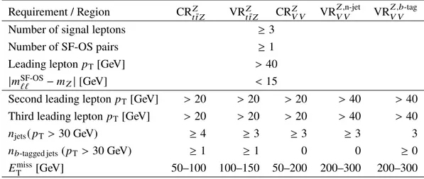
The two dedicated control regions used for the 𝑡 ¯𝑡𝑍 (CR𝑡𝑍𝑡 𝑍¯ ) and multi-boson (CR 𝑍
𝑉 𝑉) background
estimation in the 3ℓ selection are defined in Table6. To ensure mutual exclusion with the SRs, only events with 50 GeV < 𝐸miss
T
< 100 GeV are included in CR𝑍
𝑡𝑡 𝑍¯ , while a 𝑏-tagged jet veto and a
50 GeV < 𝐸missT <200 GeV requirement are applied in CR𝑍
𝑉 𝑉.
To validate the background estimates and provide a statistically independent cross-check of the extrapolation
Table 5: Background fit results for the FNP validation regions. The ‘Others’ category is dominated by 𝑡 ¯𝑡𝑊 production and also contains the contributions from 𝑡 ¯𝑡ℎ, 𝑡 ¯𝑡𝑊𝑊 , 𝑡 ¯𝑡𝑡, 𝑡 ¯𝑡𝑡 ¯𝑡, 𝑊 ℎ, and 𝑍 ℎ production. Combined statistical and systematic uncertainties are given. Some of the uncertainties are correlated and therefore the overall sum in quadrature does not necessarily add to the total systematic uncertainty. The number of 𝑡 ¯𝑡𝑍 and multi-boson background events is estimated as described in Section5.2.
VR𝑍1F VR𝑍2F
Observed events 84 98
Total (post-fit) SM events 104 ± 28 98 ± 33 Post-fit, multi-boson 0.7 ± 0.2 2.7 ± 0.7
Post-fit, 𝑡 ¯𝑡𝑍 9.1 ± 1.7 2.6 ± 0.6
Fake/non-prompt leptons 54 ± 27 76 ± 33
𝑡 𝑍, 𝑡𝑊 𝑍 0.9 ± 0.5 0.40 ± 0.21
Others 39 ± 6 16.2 ± 3.1
the 𝑡 ¯𝑡𝑍 background estimate. The VR
𝑍,n-jet
𝑉 𝑉 and VR
𝑍,𝑏-tag
𝑉 𝑉 regions validate the multi-boson background
estimate, the former focusing on the extrapolation in jet multiplicity and the latter releasing the 𝑏-tagged jet veto. The overlap between these multi-boson VRs is around 50%.
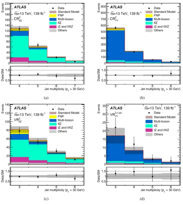
Table7shows the observed and expected yields in the CRs and VRs for each background source, and Figure2 shows the jet multiplicity distribution after the background fit for these CRs and VRs. The normalisation factors for the 𝑡 ¯𝑡𝑍 and multi-boson backgrounds do not differ from unity by more than 20% and the post-fit MC-simulated jet multiplicity distributions agree well with the data.
Table 6: Definition of the control and validation regions used for the 𝑡 ¯𝑡𝑍 and multi-boson background estimation.
Requirement / Region CR𝑍𝑡𝑡 𝑍¯ VR 𝑍 𝑡𝑡 𝑍¯ CR 𝑍 𝑉 𝑉 VR 𝑍,n-jet 𝑉 𝑉 VR 𝑍,𝑏-tag 𝑉 𝑉
Number of signal leptons ≥ 3
Number of SF-OS pairs ≥ 1
Leading lepton 𝑝T [GeV] > 40
|𝑚SF-OS
ℓ ℓ − 𝑚𝑍| [GeV]
< 15
Second leading lepton 𝑝T[GeV] >20 >20 >20 >40 >40
Third leading lepton 𝑝T [GeV] >20 >20 >20 >40 >40
𝑛
jets( 𝑝T > 30 GeV) ≥ 4 ≥ 3 ≥ 3 ≥ 3 3
𝑛𝑏
-tagged jets(𝑝T >30 GeV) ≥ 1 ≥ 1 0 0 ≥ 0
𝐸miss
0 20 40 60 80 100 120 140 160 180 200 220 Events Data Standard Model FNP Multi-boson Z t t tZ and tWZ Others ATLAS -1 =13 TeV, 139 fb s Z Z t t CR 4 5 6 7 > 30 GeV) T Jet multiplicity (p 0.5 1 1.5 Data/SM (a) 0 100 200 300 400 500 600 700 800 900 Events Data Standard Model FNP Multi-boson Z t t tZ and tWZ Others ATLAS -1 =13 TeV, 139 fb s Z VV CR 3 4 5 6 > 30 GeV) T Jet multiplicity (p 0.5 1 1.5 Data/SM (b) 0 20 40 60 80 100 120 140 Events Data Standard Model FNP Multi-boson Z t t tZ and tWZ Others ATLAS -1 =13 TeV, 139 fb s Z Z t t VR 3 4 5 6 > 30 GeV) T Jet multiplicity (p 0.5 1 1.5 Data/SM (c) 0 5 10 15 20 25 30 35 Events Data Standard Model Multi-boson Z t t tZ and tWZ Others ATLAS s=13 TeV, 139 fb-1 Z,n-jet VV VR 3 4 5 6 > 30 GeV) T Jet multiplicity (p 0.5 1 1.5 Data/SM (d)
Figure 2: Jet multiplicity distributions in control and validation regions (a) CR𝑡𝑍𝑡 𝑍¯ , (b) CR 𝑍 𝑉 𝑉, (c) VR 𝑍 𝑡𝑡 𝑍¯ and (d) VR 𝑍,n-jet
𝑉 𝑉 after normalising the 𝑡 ¯𝑡𝑍 and multi-boson background processes via the simultaneous fit described in
Section5. The contributions from all SM backgrounds are shown as a histogram stack; the bands represent the total uncertainty in the background prediction. The ‘Others’ category contains the contributions from 𝑡 ¯𝑡ℎ, 𝑡 ¯𝑡𝑊 , 𝑡 ¯𝑡𝑊𝑊 , 𝑡 ¯𝑡𝑡, 𝑡¯𝑡𝑡 ¯𝑡, 𝑊 ℎ, and 𝑍 ℎ production. The ‘FNP’ category represents the background from fake or non-prompt leptons. The last bin in each figure contains the overflow. The lower panels show the ratio of the observed data to the total SM background prediction, with bands representing the total uncertainty in the background prediction.
Table 7: Background fit results for the control and validation regions for the 𝑡 ¯𝑡𝑍 and multi-boson backgrounds. The pre-fit predictions from MC simulation are given for comparison for those backgrounds (𝑡 ¯𝑡𝑍 , multi-boson) that are normalised to data. The ‘Others’ category contains the contributions from 𝑡 ¯𝑡ℎ, 𝑡 ¯𝑡𝑊 , 𝑡 ¯𝑡𝑊𝑊 , 𝑡 ¯𝑡𝑡, 𝑡 ¯𝑡𝑡 ¯𝑡, 𝑊 ℎ, and 𝑍 ℎ production. Combined statistical and systematic uncertainties are given. Some of the uncertainties are correlated and therefore the overall sum in quadrature does not necessarily add to the total systematic uncertainty. The number of events with fake/non-prompt leptons is estimated with the data-driven technique described in Section5.1.
CR𝑡𝑍𝑡 𝑍¯ VR 𝑍 𝑡𝑡 𝑍¯ CR 𝑍 𝑉 𝑉 VR 𝑍,n-jet 𝑉 𝑉 VR 𝑍,𝑏-tag 𝑉 𝑉 Observed events 220 172 820 39 34
Total (post-fit) SM events 220 ± 15 179 ± 16 820 ± 29 30 ± 8 26 ± 6
Post-fit, multi-boson 28 ± 7 25 ± 8 698 ± 34 26 ± 8 17 ± 6 Post-fit, 𝑡 ¯𝑡𝑍 142 ± 22 105 ± 20 57 ± 11 2.8 ± 0.6 5.4 ± 1.2 Fake/non-prompt leptons 15.1 ± 1.7 16.7 ± 1.9 41 ± 15 <1.5 0.9+1.1 −0.9 𝑡 𝑍, 𝑡𝑊 𝑍 27 ± 14 23 ± 12 19 ± 10 0.9 ± 0.5 1.7 ± 0.9 Others 8.0 ± 1.4 9.7 ± 2.1 5.8 ± 1.3 0.46 ± 0.09 0.62 ± 0.12 Pre-fit, multi-boson 35.4 ± 3.5 31 ± 7 870 ± 200 32 ± 7 22 ± 5 Pre-fit, 𝑡 ¯𝑡𝑍 154 ± 14 114 ± 5 61.7 ± 3.4 3.1 ± 0.4 5.8 ± 0.6
5.3 Estimation of the 𝒕 ¯𝒕 background in the 1ℓ selection
The 𝑡 ¯𝑡 background represents more than 70% of the total background in the 1ℓ SRs and it is estimated with the aid of a dedicated control region (CR𝑡ℎ𝑡¯), defined in Table8. Compared to the SRs in Table3, this region
does not apply any selection on the number of Higgs boson candidates and features relaxed requirements on 𝑚
T, while only events with exactly four jets and 7 < S < 10 are included in this CR to ensure orthogonality
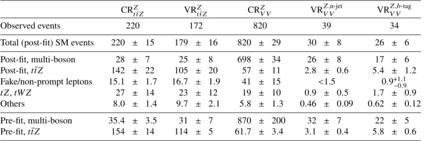
with the SRs. Table9shows the observed and expected yields in the CR for each background source, and Figure3shows the distribution of the transverse mass and number of Higgs boson candidtes after the background fit. The normalisation factor for the 𝑡 ¯𝑡 background was found to be 1.09 ± 0.13.
The extrapolation across S and 𝑚T between CR ℎ
𝑡𝑡¯ and the SRs is tested in several validation regions.
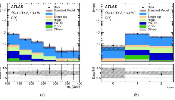
Figure4shows the definition, the observed number of events and expected yields in these regions, which feature either the same 𝑏-tagged jets multiplicity as the SRs with relaxed 𝑚T requirements, or the same
𝑚
Tselections as the SRs requiring exactly three 𝑏-tagged jets. Good agreement between the background
estimation and the data is observed in all these validation regions.
Table 8: Definition of the control region used for the 𝑡 ¯𝑡 background estimation.
Requirement / Region CRℎ𝑡𝑡¯
Number of signal leptons 1
𝑛ℎ
-cand
-𝑛𝑏
-tagged jets(𝑝T >30 GeV) ≥ 4
𝑛
jets(𝑝T >60 GeV) 4
𝑚
T[GeV] >100
1 10 2 10 3 10 4 10 Events Data Standard Model t t Single top Higgs Z t W, t t t V, VV Others ATLAS -1 =13 TeV, 139 fb s t t h CR 100 150 200 250 300 350 400 [GeV] T m 0.5 1 1.5 Data/SM (a) 1 10 2 10 3 10 4 10 Events Data Standard Model t t Single top Higgs Z t W, t t t V, VV Others ATLAS -1 =13 TeV, 139 fb s t t h CR 0 1 2 h-cand n 0.5 1 1.5 Data/SM (b)
Figure 3: (a) Transverse mass and (b) number of Higgs boson candidates distributions in CR𝑡ℎ𝑡¯after normalising the
𝑡¯𝑡 background process via the simultaneous fit described in Section5. The contributions from all SM backgrounds are shown as a histogram stack; the bands represent the total uncertainty in the background prediction. The ‘Higgs’ category contains the contributions from gluon–gluon fusion, vector-boson fusion, 𝑊 ℎ, 𝑍 ℎ and 𝑡 ¯𝑡ℎ production. The ‘Others’ category contains the contributions from 𝑡 ¯𝑡𝑊𝑊 , 𝑡 ¯𝑡𝑊 𝑍 , 𝑡 ¯𝑡𝑡 and 𝑡 ¯𝑡𝑡 ¯𝑡 production. The last bin in each figure contains the overflow. The lower panels show the ratio of the observed data to the total SM background prediction, with bands representing the total uncertainty in the background prediction.
Table 9: Background fit results for the 𝑡 ¯𝑡 background control region in the 1ℓ selection. The pre-fit predictions from MC simulation are given for comparison for those backgrounds (𝑡 ¯𝑡) that are normalised to data. The ‘Higgs’ category contains the contributions from gluon–gluon fusion, vector-boson fusion, 𝑊 ℎ, 𝑍 ℎ and 𝑡 ¯𝑡ℎ production. The ‘Others’ category contains the contributions from 𝑡 ¯𝑡𝑊𝑊 , 𝑡 ¯𝑡𝑊 𝑍 , 𝑡 ¯𝑡𝑡 and 𝑡 ¯𝑡𝑡 ¯𝑡 production. Combined statistical and systematic uncertainties are given. Some of the uncertainties are correlated and therefore the overall sum in quadrature does not necessarily add to the total systematic uncertainty.
CRℎ𝑡¯𝑡
Observed events 119
Total (post-fit) SM events 119 ± 11
Post-fit, 𝑡 ¯𝑡 105 ± 11 𝑉, 𝑉𝑉 0.6 ± 0.5 𝑡¯𝑡𝑊 , 𝑡 ¯𝑡𝑍 3.0 ± 0.7 Higgs 5.1 ± 1.8 Single top 4.6 ± 1.5 Others 0.73 ± 0.16 Pre-fit, 𝑡 ¯𝑡 96 ± 6
> 150 = 3 = 5 (7,14) > 150 = 3 6 ≥ (7,14) > 150 = 3 = 4 (10,12) > 150 = 3 = 4 (12,14) > 150 = 3 4 ≥ (> 14) (100,150) 4 ≥ 5 ≥ (> 7) (100,150) 4 ≥ = 4 (> 12) 0 0.5 1 1.5 Data/MC significance miss T E Jet multiplicity b-jet multiplicity [GeV] T m 1 10 2 10 3 10 4 10 Events
Data Standard Model t t Single top Higgs ttW, ttZ V, VV Others -1 =13 TeV, 139 fb s ATLAS
Figure 4: Comparison of the observed and expected event yields in the different kinematic regions used to validate the 𝑡 ¯𝑡 background estimation in the 1ℓ selection. The ‘Higgs’ category contains the contributions from gluon–gluon fusion, vector-boson fusion, 𝑊 ℎ, 𝑍 ℎ and 𝑡 ¯𝑡ℎ production. The ‘Others’ category contains the contributions from 𝑡¯𝑡𝑊𝑊 , 𝑡 ¯𝑡𝑊 𝑍, 𝑡 ¯𝑡𝑡 and 𝑡 ¯𝑡𝑡 ¯𝑡 production. The lower panel shows the ratio of the observed data to the total SM background prediction, with bands representing the total uncertainty in the background prediction.
6 Systematic uncertainties
The main sources of systematic uncertainty affecting the analysis SRs are related to the theoretical and modelling uncertainties in the background, the limited number of events in the CRs and MC simulated samples, the uncertainties in the FNP probabilities, as well as the jet energy scale and resolution. The effects of the systematic uncertainties are evaluated for all signal samples and background processes. Since the normalisation of the dominant background processes is extracted in dedicated CRs, the systematic uncertainties only affect the extrapolation to the SRs in these cases. Figure5summarises the contributions from the different sources of systematic uncertainty to the total SM background predictions in the signal regions.
The jet energy scale and resolution uncertainties are derived as a function of the 𝑝Tand 𝜂 of the jet, as
well as of the pile-up conditions and the jet flavour composition (more like a quark or a gluon) of the selected jet sample. They are determined using a combination of data and simulated event samples, through measurements of the jet response asymmetry in dijet, 𝑍 +jet and 𝛾+jet events [67,84].
Systematic uncertainties in the 𝑏-tagging efficiency are estimated by varying the 𝜂-, 𝑝T- and
flavour-dependent scale factors applied to each jet in the simulation within a range that reflects the systematic uncertainty in the measured tagging efficiency and mis-tag rates in data [71–73].
Other detector-related systematic uncertainties, such as those related to the 𝐸Tmissmodelling, as well as lepton reconstruction efficiency, energy scale and energy resolution are found to have a small impact on the results.
1A h SR SR1Bh 1A Z SR SR1BZ 2A Z SR SR2BZ 0 0.05 0.1 0.15 0.2 0.25 0.3 0.35 0.4 Relative Uncertainty Total uncertainty Background normalisation FNP probabilities MC and FNP statistics Theory and modelling Detector
ATLAS
-1
=13 TeV, 139 fb s
Figure 5: Comparison of the relative uncertainty for the total background yield in each SR, including the contribution from the different sources of uncertainty. The ‘Detector’ category contains all detector-related systematic uncertainties and is dominated by jet energy scale and resolution, and 𝑏-tagging uncertainties.
Systematic uncertainties are assigned to the FNP background estimation to account for different compositions (heavy flavour, light flavour or conversions) between the signal and control regions, as well as the contamination from prompt leptons in the regions used to measure the FNP probabilities.
The diboson background MC modelling uncertainties are estimated by varying the renormalisation, factorisation and resummation scales used to generate the samples [30]. For the 𝑡 ¯𝑡𝑍 background, uncertainties due to parton shower and hadronisation modelling are evaluated by comparing the predictions from MG5_aMC@NLO interfaced to Pythia and Herwig 7.0.4 [85], while the uncertainties related to the choice of renormalisation and factorisation scales are assessed by varying the corresponding event generator parameters up and down by a factor of two around their nominal values [31]. For the 𝑡 ¯𝑡 background, uncertainties due to parton shower and hadronisation modelling are evaluated by comparing the predictions from Powheg-Box interfaced to Pythia and Herwig 7.0.4 [85], while the uncertainties due the choice of generator are evaluated by comparing the predictions from Powheg-Box and MG5_aMC@NLO both interfaced to Pythia. Variations of the 𝑡 ¯𝑡 initial- and final-state radiation, renormalisation and factorisation scales are also considered [86].
The cross-sections used to normalise the MC samples are varied according to the uncertainty in the cross-section calculation, i.e. 6% for diboson, 12% for 𝑡 ¯𝑡𝑍 , 13% for 𝑡 ¯𝑡𝑊 [34] and 5% for single top production. For 𝑡 ¯𝑡𝑊𝑊 , 𝑡 𝑍 , 𝑡𝑊 𝑍 , 𝑡 ¯𝑡ℎ, 𝑊 ℎ, 𝑍 ℎ, 𝑡 ¯𝑡𝑡, 𝑡 ¯𝑡𝑡 ¯𝑡, and triboson production processes, which constitute a small background, a 50% uncertainty in the event yields is assumed.
7 Results
The observed number of events and expected yields are shown in Tables10and11for each of the inclusive 3ℓ and 1ℓ SRs, respectively. Figures6 and 7 show kinematic distributions after applying all the SR selection requirements except those on 𝐸Tmiss, 𝑝ℓ ℓT or S and jet multiplicity. The data agree with the SM background predictions and these results are interpreted as exclusion limits for several beyond-the-SM (BSM) scenarios.
The HistFitter framework, which utilises a profile-likelihood-ratio test statistic [80], is used to estimate 95% confidence intervals using the CLsprescription [87]. The likelihood is built from the product of
probability density functions describing the observed numbers of events in the SR and the associated CRs. The statistical uncertainties in the CRs and SRs are modelled using Poisson distributions. Systematic uncertainties enter the likelihood as nuisance parameters that are constrained by Gaussian distributions whose widths correspond to the sizes of these uncertainties. Table10also shows upper limits (at the 95% CL) on the number of BSM events 𝑆95, and on the visible BSM cross-section 𝜎vis= 𝑆obs95/
∫
Ld𝑡, defined as the product of the production cross-section, acceptance and efficiency.
Model-dependent limits are also set in specific classes of SUSY models. For each signal hypothesis, the background fit is repeated taking into account the signal contamination in the CRs, which is found to be below 12% for signal models close to the existing exclusion limits [20]. Correlations of the uncertainties between the SM backgrounds and the signals are taken into account.
To enhance the exclusion power in the SUSY models considered, a ‘shape-fit’ approach is used where several mutually exclusive bins in different kinematic variables are defined in order to take advantage of the different signal-to-background ratios in the different bins. Table12shows the definition of these bins, which loosen a few of the requirements of the discovery SRs to increase the acceptance for different classes of models across the phase space (Tables2and3). SR𝑍2Ais used in the exclusion fits with no changes. The observed number of events and expected yields in all these bins are shown in Figures8and9.
50 100 150 200 250 300 350 400 [GeV] miss T E 10 20 30 40 50 60 Events / 50 GeV Data Standard Model FNP Multi-boson Z t t tZ and tWZ Others ) = 650 0 2 χ∼ ) = 900, m( 1 t ~ m( ATLAS s=13 TeV, 139 fb-1 Z 1A SR (a) 0 100 200 300 400 500 600 700 [GeV] ll T p 2 4 6 8 10 12 14 16 18 Events / 150 GeV Data Standard Model FNP Multi-boson Z t t tZ and tWZ Others ) = 130 0 2 χ∼ ) = 800, m( 1 t ~ m( ATLAS s=13 TeV, 139 fb-1 Z 1B SR (b) 60 80 100 120 140 160 180 200 220 240 [GeV] miss T E 10 20 30 40 50 60 70 Events / 50 GeV Data Standard Model FNP Multi-boson Z t t tZ and tWZ Others ) = 350 0 1 χ∼ ) = 500, m( 2 t ~ m( ATLAS s=13 TeV, 139 fb-1 Z 2A SR (c) 50 100 150 200 250 300 350 400 450 [GeV] ll T p 2 4 6 8 10 12 14 Events / 100 GeV Data Standard Model FNP Multi-boson Z t t tZ and tWZ Others ) = 400 0 1 χ∼ ) = 800, m( 2 t ~ m( ATLAS s=13 TeV, 139 fb-1 Z 2B SR (d)
Figure 6: Distributions of (a) 𝐸Tmissin SR1A𝑍 , (b) 𝑝ℓ ℓT in SR𝑍1B, (c) 𝐸Tmissin SR2A𝑍 , and (d) 𝑝ℓ ℓT in SR𝑍2Bfor events passing all the SR requirements except those on the variable being plotted (the requirements are indicated by the arrows). The contributions from all SM backgrounds are shown after the background fit described in Section5; the hashed bands represent the total uncertainty. The ‘Others’ category contains the contributions from 𝑡 ¯𝑡ℎ, 𝑡 ¯𝑡𝑊 , 𝑡 ¯𝑡𝑊𝑊 , 𝑡¯𝑡𝑡, 𝑡 ¯𝑡𝑡 ¯𝑡, 𝑊 ℎ, and 𝑍 ℎ production. The ‘FNP’ category represents the background from fake or non-prompt leptons. The expected distributions for selected signal models are also shown as dashed lines. The last bin in each figure contains the overflow.
8 9 10 11 12 13 14 15 16 17 18 significance miss T E 10 20 30 40 50 60 70 Events Data Standard Model t t Single top Higgs Z t W, t t t V, VV Others ) = 750 0 2 χ∼ ) = 1000, m( 1 t ~ m( ATLAS s=13 TeV, 139 fb-1 h 1A SR (a) 4 5 6 7 > 60 GeV) T Jet multiplicity (p 10 20 30 40 50 60 70 80 90 Events Data Standard Model t t Single top Higgs Z t W, t t t V, VV Others ) = 130 0 2 χ∼ ) = 800, m( 1 t ~ m( ATLAS s=13 TeV, 139 fb-1 h 1B SR (b)
Figure 7: Distributions of (a) 𝐸Tmisssignificance in SRℎ1A and (b) jet multiplicity in SRℎ1B, for events passing all the SR requirements except those on the variable being plotted (the requirements are indicated by the arrows). The contributions from all SM backgrounds are shown after the background fit described in Section5; the hashed bands represent the total uncertainty. The ‘Higgs’ category contains the contributions from gluon–gluon fusion, vector-boson fusion, 𝑊 ℎ, 𝑍 ℎ and 𝑡 ¯𝑡ℎ production. The ‘Others’ category contains the contributions from 𝑡 ¯𝑡𝑊𝑊 , 𝑡¯𝑡𝑊 𝑍 , 𝑡 ¯𝑡𝑡 and 𝑡 ¯𝑡𝑡 ¯𝑡 production. The expected distributions for selected signal models are also shown as dashed lines. The last bin in each figure contains the overflow.
Table 10: Observed and expected numbers of events in the 3ℓ signal regions. The pre-fit predictions from MC simulation are given for comparison for those backgrounds (𝑡 ¯𝑡𝑍 , multi-boson) that are normalised to data in dedicated control regions. The ‘Others’ category is dominated by 𝑡 ¯𝑡𝑊 production and also contains the contributions from 𝑡 ¯𝑡ℎ, 𝑡¯𝑡𝑊𝑊 , 𝑡 ¯𝑡𝑡, 𝑡 ¯𝑡𝑡 ¯𝑡, 𝑊 ℎ, and 𝑍 ℎ production. Combined statistical and systematic uncertainties are given. The table also includes model-independent 95% CL upper limits on the visible number of BSM events (𝑆95obs), the number of BSM events given the expected number of background events (𝑆95exp) and the visible BSM cross-section (𝜎vis), as well as
the discovery 𝑝-value (𝑝0) for the background-only hypothesis, all calculated from pseudo-experiments. The value
of 𝑝0is capped at 0.5 if the observed number of events is below the expected number of events.
SR𝑍1A SR𝑍1B SR𝑍2A SR𝑍2B
Observed events 3 14 3 6
Total (post-fit) SM events 5.7 ± 1.0 12.1 ± 2.0 5.6 ± 1.6 5.5 ± 0.9
Post-fit, multi-boson 0.49 ± 0.22 1.5 ± 0.5 2.6 ± 1.0 1.4 ± 0.6
Post-fit, 𝑡 ¯𝑡𝑍 2.8 ± 0.9 7.9 ± 1.9 0.70 ± 0.23 2.2 ± 0.7
Fake or non-prompt leptons 0.74 ± 0.24 0.04 ± 0.02 1.8 ± 1.1 0.65 ± 0.12
𝑡 𝑍, 𝑡𝑊 𝑍 0.8 ± 0.4 2.2 ± 1.2 0.19 ± 0.10 1.0 ± 0.5 Others 0.84 ± 0.18 0.51 ± 0.11 0.25 ± 0.07 0.19 ± 0.04 Pre-fit, multi-boson 0.61 ± 0.23 1.9 ± 0.5 3.3 ± 0.9 1.8 ± 0.7 Pre-fit, 𝑡 ¯𝑡𝑍 3.0 ± 0.7 8.5 ± 1.6 0.76 ± 0.21 2.4 ± 0.5 𝑆95 obs 4.5 11.7 4.9 7.0 𝑆95 exp 6.2+2.6−1.6 9.2+4.1−1.3 6.1+2.6−1.7 6.6+2.5−1.8 𝜎 vis[fb] 0.03 0.08 0.03 0.05 𝑝 0 0.50 0.31 0.50 0.4
Table 11: Observed and expected numbers of events in the 1ℓ signal regions. The pre-fit predictions from MC simulation are given for comparison for the 𝑡 ¯𝑡 background that is normalised to data in a dedicated control region. The ‘Higgs’ category contains the contributions from gluon–gluon fusion, vector-boson fusion, 𝑊 ℎ, 𝑍 ℎ and 𝑡 ¯𝑡ℎ production. The ‘Others’ category contains the contributions from 𝑡 ¯𝑡𝑊𝑊 , 𝑡 ¯𝑡𝑊 𝑍 , 𝑡 ¯𝑡𝑡 and 𝑡 ¯𝑡𝑡 ¯𝑡 production. Combined statistical and systematic uncertainties are given. The table also includes model-independent 95% CL upper limits on the visible number of BSM events (𝑆95obs), the number of BSM events given the expected number of background events (𝑆95exp) and the visible BSM cross-section (𝜎vis), as well as the discovery 𝑝-value (𝑝0) for the background-only
hypothesis, all calculated from pseudo-experiments. The value of 𝑝0 is capped at 0.5 if the observed number of
events is below the expected number of events.
SRℎ1A SRℎ1B
Observed events 11 24
Total (post-fit) SM events 17 ± 3 19 ± 5
Post-fit, 𝑡 ¯𝑡 12 ± 3 15 ± 5 𝑉, 𝑉𝑉 0.05 ± 0.05 0.13 ± 0.08 𝑡¯𝑡𝑊 , 𝑡 ¯𝑡𝑍 1.16 ± 0.26 0.95 ± 0.25 Higgs 1.19 ± 0.21 0.9 ± 0.4 Single top 1.38 ± 0.23 0.74 ± 0.22 Others 0.68 ± 0.13 1.53 ± 0.32 Pre-fit, 𝑡 ¯𝑡 11.0 ± 2.4 14 ± 4 𝑆95 obs 7.0 18.1 𝑆95 exp 10.3+4.4−3.2 14.2+6.0−3.8 𝜎vis[fb] 0.05 0.13 𝑝 0 0.50 0.25
Table 12: Selection criteria used in the shape-fit to derive the model-dependent exclusion limits. The additional SR labelled as SRℎ1ABoverlaps with both SRℎ1Aand SRℎ1Bdefined in Table3.
SR1A𝑍 𝐸miss T [GeV] 200–250, 250–300, 300–350, >350 SR1B𝑍 𝑝ℓ ℓ T [GeV] 150–300, 300–450, 450–600, >600 SR2B𝑍 𝐸miss T [GeV] 300–350, >350 𝑝ℓ ℓ T [GeV] 50–150, >150 SRℎ1A 𝑛ℎ -cand 1, ≥2 𝑛 jets(𝑝T >60 GeV) 4 S 10–12, 12–14 SRℎ1B 𝑛ℎ-cand 1, ≥2 𝑛 jets(𝑝T >60 GeV) 5, ≥6 S 7–14 SRℎ1AB 𝑛ℎ-cand ≥1 𝑛 jets(𝑝T >60 GeV) ≥4 S ≥14 -(200,250) -(250,300) -(300,350) -> 350 (150,300) > 150 (300,450) > 150 (450,600) > 150 > 600 > 150 < 50 > 200 (50,150) (300,350) > 150 (300,350) (50,150) > 350 > 150 > 350 2 − 0 2 Significance [GeV] ll T p [GeV] miss T E 2 4 6 8 10 12 14 16 Events
Data Standard Model
FNP Multi-boson Z t t tZ and tZW Others -1 =13 TeV, 139 fb s ATLAS Z 1A SR Z 1B SR Z 2A SR Z 2B SR
Figure 8: Comparison of the observed and expected event yields in all the 3ℓ SRs and bins used for the model-dependent exclusion limits. The ‘Others’ category contains the contributions from 𝑡 ¯𝑡ℎ, 𝑡 ¯𝑡𝑊 , 𝑡 ¯𝑡𝑊𝑊 , 𝑡 ¯𝑡𝑡, 𝑡 ¯𝑡𝑡 ¯𝑡, 𝑊 ℎ, and 𝑍 ℎproduction. The ‘FNP’ category represents the background from fake or non-prompt leptons. The lower panel shows the significance in each SR bin, computed as described in Ref. [88].
= 1 = 4 (10,12) 2 ≥ = 4 (10,12) = 1 = 4 (12,14) 2 ≥ = 4 (12,14) = 1 = 5 (7,14) 2 ≥ = 5 (7,14) = 1 6 ≥ (7,14) 2 ≥ 6 ≥ (7,14) 1 ≥ 4 ≥ >14 2 − 0 2 Significance significance miss T E Jet multiplicity Higgs multiplicity 5 10 15 20 25 30 35 40 45 Events
Data Standard Model t t Single top Higgs ttW, ttZ V, VV Others -1 =13 TeV, 139 fb s ATLAS h 1A SR h 1B SR h 1AB SR
Figure 9: Comparison of the observed and expected event yields in all the 1ℓ SRs and bins used for the model-dependent exclusion limits. The ‘Higgs’ category contains the contributions from gluon–gluon fusion, vector-boson fusion, 𝑊 ℎ, 𝑍 ℎ and 𝑡 ¯𝑡ℎ production. The ‘Others’ category contains the contributions from 𝑡 ¯𝑡𝑊𝑊 , 𝑡 ¯𝑡𝑊 𝑍 , 𝑡 ¯𝑡𝑡 and 𝑡 ¯𝑡𝑡 ¯𝑡 production. The lower panel shows the significance in each SR bin, computed as described in Ref. [88].
Figure10shows the exclusion limits in the ˜𝑡1 → 𝑡 ˜𝜒 0
2 with ˜𝜒 0
2 → ℎ/𝑍 ˜𝜒 0
1 simplified model with 50%
branching ratios to each ˜𝜒0
2 decay mode. These results are obtained from the statistical combination of the
shape-fit bins of SR𝑍1A, SR1B𝑍 , SRℎ1A, SR1Bℎ and SRℎ1ABshown in Table12. The bins of SRℎ1A, SR1Bℎ and SR1ABℎ are separately combined with the bins of SR1A𝑍 and SR1B𝑍 . For each combination of sparticle masses, only the option among those two with best expected sensitivity is considered for the final limit setting. The change in best expected combination is responsible for the kink at ˜𝑡1masses of about 900–1000 GeV and
˜ 𝜒0
2masses below 200 GeV. For ˜
𝜒0
2masses above 225 GeV, ˜𝑡1masses up to about 1100 GeV are excluded at
95% CL, while ˜𝑡1masses below 1220 GeV are excluded for a ˜𝜒 0
2mass of 925 GeV. These results improve
upon the existing limits on the ˜𝑡1mass in this model by approximately 300 GeV [20].
The same statistical combination strategy is also used to obtain exclusion limits in the ˜𝑡1 → 𝑡 ˜𝜒 0 2 with ˜ 𝜒0 2 → ℎ/𝑍 ˜𝜒 0
1 simplified model for different ˜𝜒 0
2 → ℎ/𝑍 ˜𝜒 0
1 decay branching ratios, shown in Figure11.
For ˜𝜒0
2 masses above 300 GeV, the exclusion limits on ˜𝑡1masses vary by at most 40 GeV depending on
the ˜𝜒0
2 → ℎ/𝑍 ˜𝜒 0
1 branching ratios. However, for ˜𝜒 0
2 masses below 200 GeV the exclusion limits on ˜𝑡1
masses are up to 300 GeV better for models featuring only ˜𝜒0
2 → 𝑍 ˜𝜒 0
1 decays compared with models only
considering the ˜𝜒02 → ℎ ˜
𝜒0
600 700 800 900 1000 1100 1200 1300 ) [GeV] 1 t ~ m( 200 400 600 800 1000 1200 ) [GeV] 0 χ∼ 2 m( ) exp σ 1 ± Expected Limit ( ) theory SUSY σ 1 ± Observed Limit ( (arXiv:1706.03986) -1 ATLAS, 36.1 fb ) = m(t) 0 2 χ ∼ , 1 t ~ m( ∆ ) = 50% 0 1 χ∼ h + → 0 2 χ∼ ( B ) = 0 1 χ∼ Z + → 0 2 χ∼ ( B ) = 0 GeV, 0 1 χ∼ , m( 0 1 χ∼ Z/h + → 0 2 χ∼ , 0 2 χ∼ t + → 1 t ~ production, 1 t ~ 1 t ~ All limits at 95% CL -1 =13 TeV, 139 fb s ATLAS
Figure 10: Exclusion limits at 95% CL on the masses of the ˜𝑡1 and ˜𝜒 0 2, for a fixed 𝑚 ( ˜𝜒 0 1) = 0 GeV, assuming B ( ˜𝜒0 2 → 𝑍 ˜𝜒 0 1) = 0.5 and B( ˜𝜒 0 2 → ℎ ˜𝜒 0
1) = 0.5. The dashed line and the shaded band are the expected limit and its
±1𝜎 uncertainty, respectively. The thick solid line is the observed limit for the central value of the signal cross-section. The expected and observed limits do not include the effect of the theoretical uncertainties in the signal cross-section. The dotted lines show the effect on the observed limit of varying the signal cross-section by ±1𝜎 of the theoretical uncertainty. Results are compared with the observed limits obtained by the previous ATLAS search in Ref. [20].
600 700 800 900 1000 1100 1200 1300 ) [GeV] 1 t ~ m( 200 400 600 800 1000 1200 ) [GeV] 0 χ∼ 2 m( ) = 0% 0 1 χ∼ h → 0 2 χ∼ ( B ) = 50% 0 1 χ∼ h → 0 2 χ∼ ( B ) = 100% 0 1 χ∼ h → 0 2 χ∼ ( B Expected limits Observed limits ) = m(t) 0 2 χ ∼ , 1 t ~ m( ∆ ) = 0 GeV 0 1 χ∼ , m( 0 1 χ∼ Z/h + → 0 2 χ∼ , 0 2 χ∼ t + → 1 t ~ production, 1 t ~ 1 t ~ All limits at 95% CL -1 =13 TeV, 139 fb s ATLAS
Figure 11: Exclusion limits at 95% CL on the masses of the ˜𝑡1 and ˜𝜒 0
2, for a fixed 𝑚 ( ˜𝜒 0
1) = 0 GeV and different
values of B ( ˜𝜒20→ ℎ ˜𝜒 0 1) with B( ˜𝜒 0 2 → 𝑍 ˜𝜒 0 1) = 1 − B( ˜𝜒 0 2 → ℎ ˜𝜒 0
1). The dashed and solid lines are the expected and
observed limits for the central value of the signal cross-section, respectively. The expected and observed limits do not include the effect of the theoretical uncertainties in the signal cross-section.
Figure12shows the exclusion limits in the ˜𝑡2 → 𝑍 ˜𝑡1 with ˜𝑡1 → 𝑏 𝑓 𝑓 0𝜒˜0
1 simplified model for a mass
difference between the ˜𝑡1and ˜𝜒 0
1 of 40 GeV. Several options for the ˜𝑡1and ˜𝜒 0
1 mass difference are also
considered and the sensitivity is found to appreciably decrease only for values below 20 GeV. These results are obtained from the statistical combination of SR2A𝑍 and the shape-fit bins of SR𝑍2Bshown in Table12. The shape of the contour is driven by SR𝑍2Aand SR𝑍2Bbeing most sensitive to small and large mass splittings between the ˜𝑡2and the ˜𝜒
0
1respectively. Masses of the ˜𝑡2up to 875 GeV are excluded at 95% CL for a ˜𝜒 0 1
mass of about 350 GeV and ˜𝜒10masses of approximately 520 (450) GeV are excluded for ˜𝑡2masses of 650
(800) GeV, extending beyond the previous limits on the ˜𝜒10mass from Ref. [89] by up to 160 GeV.
500 600 700 800 900 1000 ) [GeV] 2 t ~ m( 300 350 400 450 500 550 600 ) [GeV] 0 χ∼ 1 m( ) exp σ 1 ± Expected Limit ( ) theory SUSY σ 1 ± Observed Limit ( ) = m(Z)1 t ~, 2 t ~ m( ∆ ) = 40 GeV 0 1 χ∼ , 1 t ~ m( ∆ , 0 1 χ∼ bff → 1 t ~ , 1 t ~ Z + → 2 t ~ production, 2 t ~ 2 t ~ All limits at 95% CL -1 =13 TeV, 139 fb s ATLAS
Figure 12: Exclusion limits at 95% CL on the masses of the ˜𝑡2and ˜𝜒 0
1, for a fixed 𝑚 ( ˜𝑡1) − 𝑚 ( ˜𝜒 0
1) = 40 GeV and
assuming B ( ˜𝑡2→ 𝑍 ˜𝑡1) = 1. The dashed line and the shaded band are the expected limit and its ±1𝜎 uncertainty,
respectively. The thick solid line is the observed limit for the central value of the signal cross-section. The expected and observed limits do not include the effect of the theoretical uncertainties in the signal cross-section. The dotted lines show the effect on the observed limit of varying the signal cross-section by ±1𝜎 of the theoretical uncertainty.
8 Conclusion
A search for direct top squark pair production in events with a leptonically decaying 𝑍 boson or a SM Higgs boson decaying into a 𝑏-quark pair is presented. The analysis uses 139 fb−1of proton–proton collision data at
√
𝑠 = 13 TeV recorded by the ATLAS detector at the LHC. No excess over the SM background predictions is observed, and exclusion limits are presented for a selection of simplified models. The limits exclude, at 95% confidence level, ˜𝑡1masses up to 1220 GeV in models featuring ˜𝑡1production and ˜𝑡1→ 𝑡 ˜𝜒
0 2
with ˜𝜒02 → 𝑍/ℎ ˜
𝜒0
1decays, and ˜𝑡2masses up to 875 GeV in models featuring ˜𝑡2production and ˜𝑡2→ 𝑍 ˜𝑡1
with ˜𝑡1→ 𝑏 𝑓 𝑓 0𝜒˜0
1 decays. Compared with previous limits, these results extend the mass parameter space
exclusion by up to 300 GeV in ˜𝑡1mass and by up to 160 GeV in ˜𝜒 0
Acknowledgements
We thank CERN for the very successful operation of the LHC, as well as the support staff from our institutions without whom ATLAS could not be operated efficiently.
We acknowledge the support of ANPCyT, Argentina; YerPhI, Armenia; ARC, Australia; BMWFW and FWF, Austria; ANAS, Azerbaijan; SSTC, Belarus; CNPq and FAPESP, Brazil; NSERC, NRC and CFI, Canada; CERN; CONICYT, Chile; CAS, MOST and NSFC, China; COLCIENCIAS, Colombia; MSMT CR, MPO CR and VSC CR, Czech Republic; DNRF and DNSRC, Denmark; IN2P3-CNRS and CEA-DRF/IRFU, France; SRNSFG, Georgia; BMBF, HGF and MPG, Germany; GSRT, Greece; RGC and Hong Kong SAR, China; ISF and Benoziyo Center, Israel; INFN, Italy; MEXT and JSPS, Japan; CNRST, Morocco; NWO, Netherlands; RCN, Norway; MNiSW and NCN, Poland; FCT, Portugal; MNE/IFA, Romania; MES of Russia and NRC KI, Russia Federation; JINR; MESTD, Serbia; MSSR, Slovakia; ARRS and MIZŠ, Slovenia; DST/NRF, South Africa; MINECO, Spain; SRC and Wallenberg Foundation, Sweden; SERI, SNSF and Cantons of Bern and Geneva, Switzerland; MOST, Taiwan; TAEK, Turkey; STFC, United Kingdom; DOE and NSF, United States of America. In addition, individual groups and members have received support from BCKDF, CANARIE, Compute Canada and CRC, Canada; ERC, ERDF, Horizon 2020, Marie Skłodowska-Curie Actions and COST, European Union; Investissements d’Avenir Labex, Investissements d’Avenir Idex and ANR, France; DFG and AvH Foundation, Germany; Herakleitos, Thales and Aristeia programmes co-financed by EU-ESF and the Greek NSRF, Greece; BSF-NSF and GIF, Israel; CERCA Programme Generalitat de Catalunya and PROMETEO Programme Generalitat Valenciana, Spain; Göran Gustafssons Stiftelse, Sweden; The Royal Society and Leverhulme Trust, United Kingdom. The crucial computing support from all WLCG partners is acknowledged gratefully, in particular from CERN, the ATLAS Tier-1 facilities at TRIUMF (Canada), NDGF (Denmark, Norway, Sweden), CC-IN2P3 (France), KIT/GridKA (Germany), INFN-CNAF (Italy), NL-T1 (Netherlands), PIC (Spain), ASGC (Taiwan), RAL (UK) and BNL (USA), the Tier-2 facilities worldwide and large non-WLCG resource providers. Major contributors of computing resources are listed in Ref. [90].