Biomedical term extraction: overview and a new methodology

(1)

HAL Id: lirmm-01274539

https://hal-lirmm.ccsd.cnrs.fr/lirmm-01274539

Submitted on 16 Feb 2016

HAL is a multi-disciplinary open access

archive for the deposit and dissemination of

sci-entific research documents, whether they are

pub-lished or not. The documents may come from

teaching and research institutions in France or

abroad, or from public or private research centers.

L’archive ouverte pluridisciplinaire HAL, est

destinée au dépôt et à la diffusion de documents

scientifiques de niveau recherche, publiés ou non,

émanant des établissements d’enseignement et de

recherche français ou étrangers, des laboratoires

publics ou privés.

Biomedical term extraction: overview and a new

methodology

Juan Antonio Lossio-Ventura, Clement Jonquet, Mathieu Roche, Maguelonne

Teisseire

To cite this version:

Juan Antonio Lossio-Ventura, Clement Jonquet, Mathieu Roche, Maguelonne Teisseire. Biomedical

term extraction: overview and a new methodology. Information Retrieval Journal, Springer, 2016,

Medical Information Retrieval, 19 (1), pp.59-99. �10.1007/s10791-015-9262-2�. �lirmm-01274539�

(2)

Biomedical Term Extraction: Overview and a New

Methodology

Juan Antonio Lossio-Ventura · Clement Jonquet · Mathieu Roche · Maguelonne Teisseire.

Received: date / Accepted: date

Abstract Terminology extraction is an essential task in domain knowledge acquisition, as well as for Information Retrieval (IR). It is also a mandatory first step aimed at building/enriching terminologies and ontologies. As often proposed in the literature, existing terminology extraction methods feature lin-guistic and statistical aspects and solve some problems related (but not com-pletely) to term extraction, e.g. noise, silence, low frequency, large-corpora, complexity of the multi-word term extraction process. In contrast, we propose a cutting edge methodology to extract and to rank biomedical terms , covering the all mentioned problems. This methodology o↵ers several measures based on linguistic, statistical, graphic and web aspects. These measures extract and rank candidate terms with excellent precision: we demonstrate that they out-perform previously reported precision results for automatic term extraction, and work with di↵erent languages (English, French, and Spanish). We also demonstrate how the use of graphs and the web to assess the significance of a term candidate, enables us to outperform precision results. We evaluated our methodology on the biomedical GENIA and LabTestsOnline corpora and compared it with previously reported measures.

J.A. Lossio-Ventura

University of Montpellier, LIRMM, CNRS - Montpellier, France E-mail: juan.lossio@lirmm.fr

C. Jonquet

University of Montpellier, LIRMM, CNRS - Montpellier, France E-mail: jonquet@lirmm.fr

M. Roche

Cirad, TETIS - Montpellier, France E-mail: mathieu.roche@cirad.fr M. Teisseire

Irstea, TETIS - Montpellier, France

(3)

Keywords Automatic Term Extraction _{· Biomedical Terminology} Extrac-tion· Natural Language Processing · BioNLP · Text Mining · Web Mining · Graphs

1 Introduction

The huge amount of biomedical data available today often consists of plain text fields, e.g. clinical trial descriptions, adverse event reports, electronic health records, emails or notes expressed by patients within forums [39]. These texts are often written using a specific language (expressions and terms) of the asso-ciated community. Therefore, there is a need for formalization and cataloging of these technical terms or concepts via the construction of terminologies and ontologies [52]. These technical terms are also important for Information Re-trieval (IR), for instance when indexing documents or formulating queries. However, as the task of manually extracting terms of a domain is very long and cumbersome, researchers have striving to design automatic methods to as-sist knowledge experts in the process of cataloging the terms and concepts of a domain under the form of vocabularies, thesauri, terminologies or ontologies. Automatic Term Extraction (ATE), or Automatic Term Recognition (ATR), is a domain which aims to automatically extract technical terminology from a given text corpus. We define technical terminology as the set of terms used in a domain. Term extraction is an essential task in domain knowledge ac-quisition because the technical terminology can be used for lexicon updating, domain ontology construction, summarization, named entity recognition or, as previously mentioned, IR.

In the biomedical domain, there is a substantial di↵erence between existing resources (hereafter called terminologies or ontologies) in English, French, and Spanish. In English, there are about 9 919 000 terms associated with about 8 864 000 concepts such as those in UMLS1 _{or BioPortal [44]. Whereas in}

French there are only about 330 000 terms associated with about 160 000 con-cepts [41], and in Spanish 1 172 000 terms associated with about 1 140 000 concepts. Note the strong di↵erence in the number of ontologies and termi-nologies available in French or Spanish. This makes ATE even more important for these languages.

In biomedical ontologies, di↵erent terms may be linked to the same concept and are semantically similar with di↵erent writing, for instance “neoplasm” and “cancer” in MeSH or SNOMED-CT. Ontologies also contain terms with morphosyntaxic variants, for instance plurals like ‘‘external fistula” and “ex-ternal fistulas”, and this group of variants is linked to a preferred term. As one of our goals is to extract new terms to enrich ontologies, our approach does not normalize variant terms, mainly because normalization would lead to pe-nalization in extracting new variant terms. Technical terms are useful to gain further insight into the conceptual structure of a domain. These may be: (i)

1 _{http://www.nlm.nih.gov/research/umls/knowledge_sources/metathesaurus/}

(4)

single-word terms (simple), or (ii) multi-word terms (complex). The proposed study focuses on both cases.

Term extraction methods usually involve two main steps. The first step extracts candidate terms by unithood calculation to qualify a string as a valid term, while the second step verifies them through termhood measures to validate their domain specificity. Formally, unithood refers to the degree of strength or stability of syntagmatic combinations and collocations, and termhood is defined as the degree to which a linguistic unit is related to domain-specific concepts [26]. ATE has been applied to several domains, e.g. biomedical [34, 18, 63, 42], ecological [12], mathematical, [56], social networks [31], banking [17], natural sciences [17], information technology [42, 60], legal [60], as well as post-graduate school websites [48].

The main issues in ATE are: (i) extraction of non-valid terms (noise) or omission of terms with low frequency (silence), (ii) extraction of multi-word terms having various complex various structures, (iii) manual validation ef-forts of the candidate terms [12], and (iv) management of large-scale corpora. Inspired by our previously published results and in response to the above is-sues, we propose a cutting edge methodology to extract biomedical terms. We propose new measures and some modifications of existing baseline measures. Those measures are divided into: 1) ranking measures, and 2) re-ranking mea-sures. Our ranking measures are statistical- and linguistic-based and address issues i), ii) and iv). Our two re-ranking measures the first one called TeR-Graph is a graph-based measure which deals with issues i), ii) and iii). The second one, called WAHI, is a web-based measure which also deals with issues i), ii) and iii). The novelty of the WAHI measure is that it is web-based which has, to the best of our knowledge, never been applied within ATE approaches. The main contributions of our article are: (1) enhanced consideration of the term unithood, by computing a degree of quality for the term unithood, and, (2) consideration of the term dependence in the ATE process. The quality of the proposed methodology is highlighted by comparing the results obtained with the most commonly used baseline measures. Our evaluation experiments were conducted despite difficulties in comparing ATE measures, mainly be-cause of the size of the corpora used and the lack of available libraries as-sociated with previous studies. Our three measures improve the process of automatic extraction of domain-specific terms from text collections that do not o↵er reliable statistical evidence (i.e. low frequency).

The paper is organized as follows. We first discuss related work in Section 2. Then the methodology to extract biomedical terms is detailed in Section 3. The results are presented in Section 4, followed by discussions in Section 5. Finally, the conclusions in Section 6.

2 Related Work

Recent studies have focused on multi-word (n-grams) and single-word (uni-grams) term extraction. Term extraction techniques can be divided into four

(5)

broad categories: (i) Linguistic, (ii) Statistical, (iii) Machine Learning, and (iv) Hybrid. All of these techniques are encompassed in Text Mining approaches. Graph-based approaches have not yet been applied to ATE, although they have been successively adopted in other Information Retrieval fields and could be suitable for our purpose. Existing web techniques have not been applied to ATE but, as we will see, these techniques can be adapted for such purposes.

2.1 Text Mining approaches 2.1.1 Linguistic approaches

These techniques attempt to recover terms via linguistic pattern formation. This involves building rules to describe naming structures for di↵erent classes based on orthographic, lexical, or morphosyntactic characteristics, e.g. [20]. The main approach is to develop rules (typically manually) describing com-mon naming structures for certain term classes using orthographic or lexical clues, or more complex morpho-syntactic features. Moreover, in many cases, dictionaries of typical term constituents (e.g. terminological heads, affixes, and specific acronyms) are used to facilitate term recognition [30]. A recent study on biomedical term extraction [21] is based on linguistic patterns plus addi-tional context-based rules to extract candidate terms, which are not scored and the authors leave the term relevance decision to experts.

2.1.2 Statistical methods

Statistical techniques chiefly rely on external evidence presented through sur-rounding (contextual) information. Such approaches are mainly focused on the recognition of general terms [59]. The most basic measures are based on frequency. For instance, term frequency (tf ) counts the frequency of a term in the corpus, document frequency (df ) counts the number of documents where a term occurs, and average term frequency (atf ), which is tf_df.

A similar research topic, called Automatic Keyword Extraction (AKE), proposes to extract the most relevant words or phrases in a document us-ing automatic indexation. Keywords, which we define as a sequence of one or more words, provide a compact representation of a document’s content. Such measures can be adapted to extract terms from a corpus as well as ATE mea-sures. We take two popular AKE measures as baselines measures, i.e. Term Frequency Inverse Document Frequency (TF-IDF) [53], and Okapi BM25 [49] (hereafter Okapi ), these weight the word frequency according to their distribu-tion along the corpus. Residual inverse document frequency (RIDF) compares the document frequency to another chance model where terms with a particu-lar term frequency are distributed randomly throughout the collection, while Chi-square [37] assesses how selectively words and phrases co-occur within the same sentences as a particular subset of frequent terms in the document text. This is applied to determine the bias of word co-occurrences in the document

(6)

text, which is then used to rank words and phrases as keywords of the docu-ment; RAKE [50] hypothesises that keywords usually consist of multiple words and do not contain punctuation or stop words. It uses word co-occurrence in-formation to determine the keywords.

2.1.3 Machine Learning

Machine Learning (ML) systems are often designed for specific entity classes and thus integrate term extraction and term classification. Machine Learning systems use training data to learn features useful for term extraction and classification. But the avaibility of reliable training resources is one of the main problems. Some proposed ATE approaches use machine learning [12, 62, 42]. However, ML may also generate noise and silence. The main challenge is how to select a set of discriminating features that can be used for accurate recognition (and classification) of term instances. Another challenge concerns the detection of term boundaries, which are the most difficult to learn. 2.1.4 Hybrid methods

Most approaches combine several methods (typically linguistic and statistically based) for the term extraction task. GlossEx [29] considers the probability of a word in the domain corpus divided by the probability of the appearance of the same word in a general corpus. Moreover, the importance of the word is increased according to its frequency in the domain corpus. Weirdness [1] con-siders that the distribution of words in a specific domain corpus di↵ers from that in a general corpus. C/NC-value [18] combines statistical and linguistic information for the extraction of multi-word and nested terms. This is the most well-known measure in the literature. While most studies address specific types of entities, C/NC-value is a domain-independent method. It has also been used for recognizing terms in the biomedical literature [24, 22]. In [63], the authors showed that C-value obtains the best results compared to the other measures cited above. C-value has been also modified to extract single-word terms [40], and in this work the authors extract only terms composed of nouns. Moreover, C-value has also been applied to di↵erent languages other than English, e.g. Japanese, Serbian, Slovenian, Polish, Chinese [25], Spanish [4], Arabic, and French. We have thus chosen C-value as one of our baseline measure. Those baseline measures will be modified and evaluated with the new proposed mea-sures.

Terminology Extraction from Parallel and Comparable Corpora

Another kind of approach suggests that terminology may be extracted from parallel and/or comparable corpora. Parallel corpora contain texts and their translation into one or more languages, but such corpora are scarce [9]. Thus parallel corpora are scarce for specialized domains. Comparable corpora are those which select similar texts in more than one language or variety [15].

(7)

Comparable corpora are built more easily than parallel corpora. They are of-ten used for machine translation and their approaches are based on linguistics, statistics, machine learning, and hybrid methods. The main objective of these approaches is to extract translation pairs from parallel/comparable corpora. Di↵erent studies propose translation of biomedical terms for English-French by alignment techniques [16]. English-Greek and English-Romanian bilingual medical dictionaries are also constructed with a hybrid approach that com-bines semantic information and term alignments [28]. Other approaches are applied for single- and multi-word terms with English-French comparable cor-pora [14]. The authors use statistical methods to align elements by exploiting contextual information. Another study proposes to use graph-based label prop-agation [57]. This approach is based on a graph for each language (English and Japanese) and the application of a similarity calculus between two words in each graph. Moreover, some machine learning algorithms can be used, e.g. the logistic regression classifier [27]. There are also approaches that combine both corpora [38] (i.e. parallel and comparable) in an approach to reinforce extraction. Note that our corpora are not parallel and are far of being com-parable because of the di↵erence in their size. Therefore these approaches are not evaluated in our study.

2.1.5 Tools and applications for biomedical term extraction

There are several applications implementing some measures previously men-tioned, especially C-value for biomedical term extraction. The study of related tools revealed that most existing systems that especially implement statisti-cal methods are made to extract keywords and, to a lesser extent, to extract terminology from a text corpus. Indeed, most systems take a single text doc-ument as input, not a set of docdoc-uments (as corpus), for which the IDF can be computed. Most systems are available only in English and the most relevant for the biomedical domain are:

– TerMine2_{, developed by the authors of the C-value method, only for}

En-glish term extraction;

– Java Automatic Term Extraction3_{[63], a toolkit which implements several}

extraction methods including C-value, GlossEx, TermEx and o↵er other measures such as frequency, average term frequency, IDF, TF-IDF, RIDF ; – FlexiTerm4_{[55], a tool explicitly evaluated on biomedical copora and which}

o↵er more flexibility than C-value when comparing term candidates (treat-ing them as bag of words and ignor(treat-ing the word order);

– BioYaTeA 5 _{[21], is a version of the YaTeA term extractor [2], both are}

available as a Perl module. It is a biomedical term extractor. The method used is based only on linguistic aspects.

2 _{http://www.nactem.ac.uk/software/termine/} 3 _{https://code.google.com/p/jatetoolkit/} 4 _{http://users.cs.cf.ac.uk/I.Spasic/flexiterm/} 5 _{http://search.cpan.org/~bibliome/Lingua-BioYaTeA/}

(8)

– BioTex 6_{[32], only for biomedical terminology extraction. It is available for}

online testing and assessment but can also be used in any program as a Java library (POS tagger not included). In contrast to other existing systems, this system allows us to analyze French and Spanish corpora, manually validate extracted terms and export the list of extracted terms.

2.2 Graph-based approaches

Graph modeling is an alternative for representing information, which clearly highlights relationships of nodes among vertices. It also groups related infor-mation in a specific way, and a centrality algorithm can be applied to enhance their efficiency. Centrality in a graph is the identification of the most im-portant vertices within a graph. A host of measures have been proposed to analyze complex networks, especially in the social network domain [7, 8, 3]. Freeman [19], formalized three di↵erent measures of node centrality: degree, closeness and betweenness. Degree is the number of neighbors that a node is connected to. Closeness is the inverse sum of shortest distances to all other neighbor nodes. Betweenness is the number of shortest paths from all vertices to all others that pass through that node. One study proposes to take the number of edges and their weights into account [45], since the three last mea-sures do not do this. Another well known measure is PageRank [46], which ranks websites. Boldi [6], evaluated the behavior of ten measures, and associ-ated the centrality to the node with largest degree. Our approach proposes the opposite, i.e. we focus on nodes with a lower degree. An increasingly popular recent application of graph approaches to IR concerns social or collaborative networks and recommender systems [43, 3].

Graph representations of text and scoring function definition are two widely explored research topics, but few studies have focused on graph-based IR in terms of both document representation and weighting models [51]. First, text is modeled as a graph where nodes represent words and edges represent relations between words, defined on the basis of any meaningful statistical or linguistic relation [5]. In [5], the authors developed a graph-based word weighting model that represents each document as a graph. The importance of a word within a document is estimated by the number of related words and their importance, in the same way that PageRank [46] estimates the importance of a page via the pages that are linked to it. Another study introduces a di↵erent representation of document that captures relationships between words by using an unweighted directed graph of words with a novel scoring function [51].

In the above approaches, graphs are used to measure the influence of words in documents like automatic keyword extraction methods (AKE), while rank-ing documents against queries. These approaches di↵er from ours as they use graphs focused on the extraction of relevant words in a document and com-puting relations between words. In our proposal, a graph is built such that

(9)

the vertices are word terms and the edges are relations between multi-word terms. Moreover, we focus especially on a scoring function of relevant multi-word terms in a domain rather than in a document.

2.3 Web Mining approaches

Di↵erent web mining studies focus on semantic similarity, semantic related-ness. This means quantifying the degree to which some words are related, considering not only similarity but also any possible semantic relationship among them. The word association measures can be divided into three cate-gories [10]: (i) Co-occurrence measures that rely on co-occurrence frequencies of both words in a corpus, (ii) Distributional similarity-based measures that characterize a word by the distribution of other words around it, and (iii) Knowledge-based measures that use knowledge-sources like thesauri, semantic networks, or taxonomies [23]. In this paper, we focus on co-occurrence mea-sures because our goal is to extract multi-word terms and we suggest comput-ing a degree of association between words composcomput-ing a term. Word association measures are used in several domains like ecology, psychology, medicine, and language processing, and were recently studied in [47, 61], such as Dice, Jac-card, Overlap, Cosine. Another measure to compute the association between words using web search engines results is the Normalized Google Distance [11], which relies on the number of times words co-occur in the document indexed by an information retrieval system. In this study, experimental results with our web-based measure will be compared with the basic measures (Dice, Jaccard, Overlap, Cosine).

3 Methodology

This section describes the baseline measures, their modifications as well as new measures that we propose for the biomedical term extraction task. The principle of our approach is to assign a weight to a term, which represents the appropriateness of being a relevant biomedical term. This allows to give as output a list ranked by their appropriateness. Our methodology for automatic term extraction has three main steps plus an additional step (a), described in Figure 1, and in the sections hereafter:

(a) Pattern Construction, (1) Candidate Term Extraction, (2) Ranking of Candidate Terms, (3) Re-ranking.

Pattern Construction (step a)

As previously cited, we supposed that biomedical terms have a similar syn-tactic structure (linguistic aspect). Therefore, we built a list of the most

(10)

com-Fig. 1 Workflow Methodology for Biomedical Term Extraction.

mon linguistic patterns according to the syntactic structure of terms present in the UMLS7 _{(for English and Spanish), and the French version of MeSH}8_,

SNOMED International and the rest of the French content in the UMLS. Part-of-Speech (POS) tagging is the process of assigning each word in a text to its grammatical category (e.g. noun, adjective). This process is performed based on the definition of the word or on the context in which it appears. This is highly time-consuming, so we conducted automatic part-of-speech tagging.

We evaluated three tools (TreeTagger9_{, Stanford Tagger}10_{and Brill’s rules}11_).

This evaluation was carried out throughout the entire workflow with the three tools and we assessed the precision of the extracted terms. We noted that in general TreeTagger gave the best results for Spanish and French. Meanwhile, for English, the Stanford tagger and TreeTagger gave similar results. We fi-nally chose TreeTagger, which gave better results and may be used for English, French and Spanish. Moreover, our choice was validated with regard to a recent

7 _{http://www.nlm.nih.gov/research/umls} 8 _{http://mesh.inserm.fr/mesh/}

9 _{http://www.cis.uni-muenchen.de/~schmid/tools/TreeTagger/} 10 _{http://nlp.stanford.edu/software/tagger.shtml}

(11)

comparison study [58], wherein the authors showed that TreeTagger generally gives the best results, particularly for nouns and verbs.

Therefore, we carried out automatic part-of-speech tagging of the biomedi-cal terms using TreeTagger, and then computed the frequency of the syntactic structures. Patterns among the 200 highest frequencies were selected to build the list of patterns for each language. From this list, we also computed the weight (probability) associated with each pattern, i.e. the frequency of the pattern over the sum of frequencies (see Algorithm 1), but this weight will only be used for one measure. The number of terms used to build these lists of patterns was 3 000 000 for English, 300 000 for French, and 500 000 for Span-ish, taken from the previously mentioned terminologies. Table 1 illustrates the computation of the linguistic patterns and their weights for English.

Di↵erent terminology extraction studies are based on the use of regular expressions to extract candidate terms, for instance [18]. Generally these reg-ular expressions are manually built for a specific language and/or domain [13]. In our setting, we prefer to (i) construct and (ii) apply patterns in order to extract terms in texts. These patterns have the advantage of being generic because they are based on defined PoS tags. Moreover, they are very specific because they are (automatically) built with specialized biomedicine resources. Concerning this last point, we can consider we are close to the use of regular ex-pressions. There are two main reasons that we use specific linguistic patterns. First, we would like to restrict the patterns to the biomedical domain. For instance, biomedical terms often contain numbers in their syntactic structure, and this is very specific to the biomedical domain, e.g. “epididymal protein 9”, “pargyline 10 mg”. General patterns do not enable extraction of such terms. Our methodology is based on 200 significant patterns for English, French, or Spanish, yet di↵erent for each language. For instance, there are 55 patterns for English that contain numbers in the linguistic structure. Thus, this kind of pattern seems quite relevant for this domain. The second reason for using lexical patterns is that we assign a probability of occurrence to each pattern, which would not be possible with classical patterns and regular expressions. 3.1 Candidate Term Extraction (step 1)

The first main step is to extract the candidate terms. So we apply part-of-speech to the whole corpus using TreeTagger. Then we filter out the content of our input corpus using previously computed patterns. We select only terms whose syntactic structure is in the patterns list. The pattern filtering is specif-ically done on a per-language basis (i.e. when the text is in French, only the French list of patterns is used).

3.2 Ranking of Candidate Terms (step 2)

We need to select the most appropriate terms for the biomedical domain. Can-didate term ranking is therefore essential. For this purpose, several measures

(12)

Algorithm 1: ComputePatterns (Dictionary, np)

Data: Dictionary = dictionary of a domain, np = number of patterns to use Result: HTpatterns(pattern, probability) = Hashtable of the first np linguistic

patterns with its probability begin

HTpatterns ;;

HTaux(tag, f req) ; // Hashtable of the tag of each term with its frequency ;

sizeHT number of terms in Dictionary; f reqtotal 0 ;

probability 0.0 ; Tag of the Dictionary;

for tag of each term 2 Dictionary do if tag2 HTauxthen

update HTaux(tag, f req + 1);

else

add HTaux(tag, 1);

end end

Rank HTaux(tag, f req) by the f req;

f reqtotal Pnpi=1f req(HTaux(i));

for i = 1; i np; i++ do probability f req(HTaux(i))

f reqtotal ;

add HTpatterns(tag(HTaux(i)), probability);

end end

Pattern Frequency Probability

NN IN JJ NN IN JJ NN 3006 3006/4113 = 0.73

NN CD NN NN NN 1107 1107/4113 = 0.27

4113 1.00

Table 1 Example of pattern construction (where NN is a noun, IN a preposition or sub-ordinating conjunction, JJ an adjective, and CD a cardinal number)

are proposed and Figure 1(2) shows the set of available measures. We propose some modifications of the most known measures in the literature (i.e., C-value, TF-IDF, Okapi ), and propose new ones (i.e., F-TFIDF-C, F-OCapi, LIDF-value, L-value). Those measures are linguistic- and statistic- based, they are also not very time-consuming. In this step, only one measure will be selected to perform the ranking. The measures of this section take a list of candi-date terms previously filtered by linguistic patterns as input, which makes it possible to assess less invalid terms while dealing with the noise problem. In addition to the use of linguistic patterns to alleviate the problem of the extraction of multi-word terms having various complex structures. Moreover, the frequency decreases the number of invalid terms to evaluate (noise). The measures mentioned above are e↵ective on large amounts of data [36, 35, 54], which overcomes the problem of large-scale corpora. Hereafter we describe all measures.

(13)

3.2.1 C-value

The C-value method combines linguistic and statistical information [18]. Lin-guistic information is the use of a general regular expression as linLin-guistic pat-terns, and the statistical information is the value assigned with the C-value measure based on the frequency of terms to compute the termhood (i.e. the as-sociation strength of a term to domain concepts). The C-value method aims to improve the extraction of long terms, and it was specially built for extracting multi-word terms. C-value(A) = 8 > > > > > < > > > > > :

w(A)_{⇥ f(A)} if A /_{2 nested}

w(A)⇥ f (A) _|S1_A_|⇥ X b2SA f (b) ! otherwise (1)

Where A is the candidate term, w(A) = log2(|A|), |A| the number of words

in A, f (A) the frequency of A in the unique document, SA the set of terms

that contain A and_|SA| the number of terms in SA. In a nutshell, C-value uses

either the frequency of the term if the term is not included in other terms (first line), or decreases this frequency if the term appears in other terms, based on the frequency of those other terms (second line).

We modified the measure in order to extract all terms (single-word + multi-words terms), as also suggested in [4], but in a di↵erent manner.

The original C-value defines w(A) = log2(|A|), and we modified w(A) =

log2(|A| +1) in order to avoid null values for single-word terms, as illustrated

in Table 2. Note that we do not use a stop word list or a frequency threshold as was originally proposed.

Original C-value Modified C-value

w(A) = log2(|A|) w(A) = log2(|A| +1)

antiphospholipid antibodies

log2(2) = 1 log2(2 +1) = 1, 6

white blood log2(2) = 1 log2(2 +1) = 1, 6

platelet log2(1) =0 log2(1 +1) = 1

Table 2 Calculation of w(A)

3.2.2 TF-IDF and Okapi

These measures are used to associate a weight to each term in a document [53]. This weight represents the term relevance for the document. The output is a ranked list of terms for each document, which is often used in information retrieval so as to order documents by their importance for a given query [49].

(14)

Okapi can be seen as an improvement of the TF-IDF measure, while taking the document length into account.

T F -IDF (A, d, D) = tf (A, d)⇥ idf(A, d) (2)

tf (A, d) = f (A, d)

max{f(A, d) : w 2 d}

idf (A, d) = log |D|

|{d 2 D : A 2 d}|

Okapi(A, d, D) = tfBM 25(A, d)⇥ idfBM 25(A, d) (3)

tfBM 25(A, d) =

tf (A, d)⇥ (k1+ 1)

tf (A, d) + k1⇥ (1 b + b⇥_dldl(d)_avg))

idfBM 25(A, d) = log|D|

dc(A) + 0.5 dc(A) + 0.5

Where A is a term, considering d a document, D the collection of docu-ments, f (A, d) the frequency of A in d, tf (A, d) the term frequency of A in d, idf (A, D) the inverse document frequency of A in D, dc(t) the number of documents containing term A, this means:|{d 2 D : t 2 d}|, dl(d) the length of the document d in number of words, dlavg the average document length of

the collection.

As the output is a ranked list of terms per document, we could find the same term in di↵erent documents, with di↵erent weights in each document. So we need to merge the term into a single list. For this, we propose to merge them according to three functions, which respectively calculate the sum(S), max(M ) and average(A) of the weights of a term. At the end of this task, we have three lists from Okapi and three lists from TF-IDF. The notation for these lists are OkapiX(A) and T F -IDFX(A), where A is the term, and X the

factor_{2 {M, S, A}. For example, Okapi}M(A) is the value obtained by taking

the maximum Okapi value for a term A in the whole corpus. Figure 2 shows the merging process.

With aim of improving the term extraction precision, we designed two new combined measures, while taking the values obtained in the above steps into account. Both are based on harmonic means of two values.

3.2.3 Combinations: F-OCapi and F-TFIDF-C

Considered as the harmonic mean of the two used values, this method has the advantage of using all values of the distribution.

F -OCapiX(A) = 2⇥

OkapiX(A)⇥ C-value(A)

OkapiX(A) + C-value(A)

(4) F -T F IDF -CX(A) = 2⇥T F IDFX(A)⇥ C-value(A)

T F IDFX(A) + C-value(A)

(15)

Fig. 2 Merging lists.

3.2.4 LIDF-value and L-value

In this section we present two new measures. The first one, called LIDF-value (Linguisitic patterns, IDF, and C-LIDF-value information). LIDF-LIDF-value is partially presented in [34]. This is a new ranking measure based on linguistic and statistical information.

Our method LIDF-value is aimed at computing the termhood for each term, using the linguistic information calculated as described below, the idf, and the C-value of each term. The linguistic information gives greater im-portance to the term unithood in order to detect low frequency terms. So we associate the pattern weight (see Table 1) with the candidate term probability. That means the probability of a candidate term of being a relevant biomedical term. The probability is associated only if the syntactic structure of the term appears in the linguistic pattern list.

The inverse document frequency (idf ) is a measure indicating the extent to which a term is common or rare across all documents. It is obtained by dividing the total number of documents by the number of documents containing the term, and then by taking the logarithm of that quotient. The probability and idf improve low frequency term extraction. The objective of these two components is to tackle the silence problem, allowing extraction of discriminant terms, for instance, in a biomedical corpus, “virus production” with low frequency being better ranked than “human monocytic cell”, which has a higher frequency. This means that for a low frequency candidate term, its score can be favored if its linguistic pattern is associated with a high probability and/or its idf value is also high. The C-value measure is based on the term frequency. The C-value (see formula 1) measure favors a candidate term that does not often appear in a longer term. For instance, in a specialized corpus (Ophthalmology), the authors of [18] found the irrelevant term “soft contact” while the frequent and longer term “soft contact lens” is relevant.

As an example, we implement the Algorithm 2, which describes the ap-plied process. These di↵erent statistical information items (i.e. probability of linguisitic patterns, C-value, idf ) are combined to define the global ranking measure LIDF-value (see formula 6); where P(ALP) is the probability of a

(16)

term A which has the same linguistic structure pattern LP , i.e. the weight of the linguistic pattern LP computed in Subsection Pattern Construction.

LIDF -value(A) = P(ALP)⇥ idf(A) ⇥ C-value(A) (6)

Algorithm 2: ComputeLIDF-value (Corpus, Patterns, minf req,

numterms)

Data: Corpus = set of documents of a specific-domain;

P atterns = HTpatterns(pattern, probability) //Hashtable of linguistic patterns with

its probability;

minf req= frequency threshold for candidate terms;

numterms= number of terms to take as output

Result: Lterms= List of ranked terms

begin

Tag the Corpus;

Take the lemma of each tagged word;

Extract candidate terms A by filtering with P atterns; Remove candidate terms A below minf req;

for each candidate term A 2 Corpus do

LIDF -value(A) = P(ALP)⇥ idf(A) ⇥ C-value(A);

add A to Lterms;

end

Rank Ltermsby the value obtained with LIDF -value;

Select the first numterms terms of Lterms;

end

Note that LIDF-value works only for a set of documents, mainly because the idf measure can only be computed on a set of documents (see formula 2). Therefore, for datasets composed of one document, we propose a new measure, L-value, as explained in the following paragraphs.

L-value is a variant of LIDF-value, focused on one document with the goal of benefiting from the probability of linguisitic patterns computed for LIDF-value. This measure does not contain the idf (see formula 7).L-value is interesting to highlight the more representative terms of a single corpus with-out considering the discriminative aspects, e.g. idf. This measure gives another point of view and is complementary to those based on the idf weighting.

A single document can be considered as a free text without delimita-tion. For instance, a scientist article, a book, a document created with ti-tles/abstracts from a library database. L-value becomes interesting when it does not exist a considerable amount of data for a new subject, i.e. an emer-gent term in the community. For instance, the “Ataxia Neuropathy Spectrum” term appears only in 4 titles/abstracts of scientist articles from PubMed12

be-tween 2009 and 2015. PubMed is a free search engine accessing primarily the MEDLINE database of references and abstracts on life sciences and biomedical topics.

(17)

L-value(A) = P(ALP)⇥ C-value(A) (7)

3.3 Re-ranking (step 3)

After the term extraction, we propose new measures to re-rank the candidate terms in order to increase the top k term precision. The re-ranking measures aim to improve the term extraction results of ranking measures. This involves positioning the most relevant biomedical terms at the top of the list. That provides more confidence that the terms appearing at the top of this list are true biomedical terms.

These re-ranking functions represent an extension of the measures pre-sented in [33]. Therefore, as improvements, we propose to take graph-theoretic information into account to highlight relevant terms, as well as web informa-tion, as explained in the following subsections. These measures can be executed separately, but the graph construction is time consuming, and the number of search engine queries is limited. Therefore, we just apply these measures for a group of selected terms given by a ranking measure. Because the ranking measures have proved to be more efficient applied before than TeRGraph and web-based measures.

As these measures are applied to the list of terms obtained with a ranking measure, which tackles noise, silence and multi-word term extraction problems, so they also take into account those problems. As mentioned, the objective of re-raking measures is to re-rank terms, so the manual validation e↵orts of the candidate terms decrease because the relevant biomedical term is allocated at the top of the list.

3.3.1 A new graph-based ranking measure: “TeRGraph” (Terminology Ranking based on Graph information)

This approach aims to improve the ranking (and therefore the precision results) of extracted terms. As mentioned above, in contrast to the above-cited study, the graph is built with a list of terms obtained according to a measure described in Section 3.2, where vertices denote terms linked by their co-occurrence in sentences in the corpus. Moreover, we make the hypothesis that the term representativeness in a graph, for a specific-domain, depends on its number of neighbors, and the number of neighbors of its neighbors. We assume that a term with more neighbors is less representative of the specific domain. This means that this term is used in the general domain. Figure 3 illustrates our hypothesis.

The graph-based approach is divided into two steps:

(i) Graph construction: a graph (see Figure 5) is built where vertices denote terms, and edges denote occurrence relations between terms, co-occurrences between terms are measured as the weight of the relation in the initial corpus. This approach is statistical because it links all co-occurring

(18)

Fig. 3 Importance of a term in a domain

terms without considering their meaning or function in the text. This graph is undirected as the edges imply that terms simply co-occur, without any further distinction regarding their role. We take the Dice coefficient, a basic measure to compute the co-occurrence between two terms x and y, as defined by the following formula:

D(x, y) = 2⇥ P (x, y)

P (x) + P (y) (8)

(ii) Representativeness computations on the term graph: a principled graph-based measure to compute term weights (representativeness) is de-fined. The aim of this new graph-based ranking measure, TeRGraph, see Equation 9, is to derive these weights for each vertex, (i.e. multi-word term weight), in order to re-rank the list of extracted terms.

T eRGraph(A) = log2 0 B B B @k + 1 1 +_{|N(A)| +} X Ti2N(A) |N(Ti)| 1 C C C A (9)

Where A represents a vertex (term), N(A) the neighborhood of A, |N(A)| the number of neighbors of A, Ti the neighbor i of A, and k a constant. The

intuition for Equation 9 is as follows: the more a term A has neighbors (di-rectly with N(A) or by transitivity with N(Ti)), the more the weight decreases.

Indeed, a term A having a lot of neighbors is considered too general for the do-main (i.e. this term is not salient), so it has to be penalized via the associated score.

The k constant a↵ects the TeRGraph value, i.e. the set of values that TeRGraph takes when k changes. For instance, when k = 0.5, the set of values for TeRGraph is between 1 and 0, (i.e., T eRGraph _{2 [ 1, 0]), and when} k = 1, T eRGraph_{2 [0, 0.6]. As the values taken by TeRGraph are di↵erent,} then the slope of the curve is also di↵erent. Figure 4 shows the behavior of TeRGraph when k changes. According the experiments, we have chosen

(19)

Fig. 4 TeRGrpah’s value for k ={0.5; 1; 1.5; 2}

k = 1.5. The main reason is that the slope of the curve is low, and the set of values for TeRGraph ranges from 0.6 to 1.

See Algorithm 3 for more details, it describes the entire process: (1) co-occurrence graph construction, (2) computation of the representativeness of each vertex.

Figure 5 shows an example to calculate the value of TeRGraph for a term in di↵erent graphs. These graphs are built with di↵erent co-occurrence thresholds (i.e. Dice’s value between two terms). In this example, A1 and A2 represent

the term chloramphenicol acetyltransferase reporter in Graphs 1 and 2, respec-tively.

3.3.2 WebR

The aim of our web-based measure, to predict with a better confidence if a candidate term is a valid biomedical term or not. It is appropriated for multi-word terms, as it computes the dependence between the multi-words of a term. In our case, we compute a “strict” dependence, which means the proximity of words of terms (i.e. neighboring words) is calculated with a strict restriction. In comparison to other web-based measures [11], WebR reduces the number of pages to consider by taking only web pages containing all words of the terms into account. In addition, our measure can be easily adopted for all types of multi-word terms.

(20)

Algorithm 3: ComputeTeRGraph (Lterms, numterms, , k)

Data: Lterms= List of ranked terms;

numterms= number of terms to be evaluated;

= threshold to create an edge between two terms; k = constant;

Result: RRLterms= Re-Ranked List of terms

begin

Select all possible pairs of terms of Ltermsto compute D(x, y) // in total

C2

numterms=2! (numtermsnumterms!2)! possibilities ;

Select pairs which D(x, y) for creating an edge ; Select all terms of Ltermsto compute T eRGraph ;

for each term A2 Ltermsdo

N(A) neighborhood of A; |N(A)| number of neighbors of A;

T eRGraph(A) = log₂ 0 B B B @k + 1 1+|N(A)|+ X Ti2N(A) |N(Ti)| 1 C C C A; add A to RRLterms; end

Rank RRLtermsby the value obtained with T eRGraph;

end

Fig. 5 TeRGraph’s value for chloramphenicol acetyltransferase reporter

W ebR(A) = nb(“A”)

nb(A) (10)

Where A = multi-word term, ai 2 A and ai = {noun, adjective, foreign

word_}.

Where A is the candidate term, nb(“A”) the number of hits returned by a web search engine with exact match only with multi-word term A (query with quotation marks “A”), nb(A) the number of documents returned by the search engine, including not exact matches (query A without quotation marks), i.e. whole documents containing words of the multi-word term A. For example, the multi-word term treponema pallidum, will generate two queries, the first

(21)

nb(“treponema pallidum”) which returns with Yahoo 1 100 000 documents, and the second query nb(treponema pallidum) which returns 1 300 000 docu-ments, then WebR(treponema pallidum)= 1100000_1300000= 0.85.

In our workflow, we tested Yahoo and Bing. WebR re-rank the list of candidate terms returned by the combined measures.

3.3.3 A new web ranking measure: WAHI (Web Association based on Hits Information)

Previous studies of web mining approaches query the web via search engines to measure word associations. This enables measurement of the association of words composing a term (e.g. soft, contact, and lens that compose the relevant term soft contact lens). To measure this association, our web-mining approach takes the number of pages provided by search engines into account (i.e.number of hits).

Our web-based measure re-ranks the list obtained previously with TeR-Graph. We will show that this improves the precision of the k first terms extracted (see Section 4) and that it is specially appropriate for multi-word term extraction.

Formula 8 leads directly to formula 1113_{. The nb function used in formula}

11 represents the number of pages returned by search engines (i.e. Yahoo and Bing). With this measure, we compute a strict dependence (i.e. neighboring words by using the operator ’ ” ’ of search engines). For instance, x might represent the word soft and y the word contact in order to calculate the asso-ciation measure of the soft contact term.

Dice(x, y) = 2⇥ nb(“x y”)

nb(x) + nb(y) (11)

Then we extend this formula to n elements as follows: Dice(a1, ..., an) = n⇥ nb(“a1 ... an”) nb(a1) + ... + nb(an) = n_X⇥ nb(“A”)n i=1 nb(ai) (12)

This measure enables us to calculate a score for all multi-word terms, such as soft contact lens.

To obtain WAHI, we propose to associate Dice criteria with WebR (see formula 10). This only takes the number of web pages containing all the words of the terms into account by using operators “ ” and AND.

For example, soft contact lens, the numerator corresponds to the number of web pages with the query “soft contact lens”, and for the denominator, we consider the query soft AND contact AND lens.

13 _{by writing P (x) =} nb(x) nb total, P (y) = nb(y) nb total, P (x, y) = nb(x,y) nb total

(22)

Finally, the global ranking approach combining Dice and WebR is given by WAHI measure (Web Association based on Hits Information):

W AHI(A) = n_X⇥ nb(“A”)n

i=1

nb(ai)

⇥nb(“A”)_nb(A) (13)

Algorithm 4 details the global web mining process to rank terms. We show in the next section that open-domain (general) resources, such as the web, can be tapped to support domain-specific term extraction. They can thus be used to compensate for the unavailability of domain-specific resources.

Algorithm 4: ComputeWAHI (Lterms, numterms, LC)

Data: Lterms= List of ranked terms;

numterms= number of terms to be evaluated;

LC ={noun, adjective, foreign word} // linguistic categories Result: RRLterms= Re-Ranked List of terms

begin

Select the first numterms terms of Ltermsto compute W AHI;

for each term A2 Ltermsdo

for all words aiof A2 LC do

n number of words in A; W AHI(A) n ⇥_Xnnum-hits(“A”) i=1 num-hits(ai) ⇥num-hits(“A”)num-hits(A) ; end add A to RRLterms; end

Rank RRLtermsby the value obtained with W AHI;

end

4 Experiments and results 4.1 Data, Protocol, and Validation 4.1.1 Data

We used two corpora for our experiments. The first one is a set of biological laboratory tests, extracted from LabTestsOnline14_{. This website provides}

in-formation in several languages to patients or family caregivers about clinical lab tests. Each test that forms a document in our corpus includes the for-mal lab test name, some synonyms and possible alternate names as well as a description of the test. The LabTestsOnline website was extracted totally

(23)

for English, French, and Spanish with a crawler created specifically for this purpose. These documents are available online15_{. Table 3 shows the details of}

LabTestsOnline corpus for di↵erent languages.

Number of Clinical Tests Number of Words

English 235 377 000 words

French 137 174 000 words

Spanish 238 396 000 words

Table 3 Details of LabTestsOnline corpus.

The second corpus is GENIA16_{, which is made up of 2 000 titles and}

ab-stracts of journal articles that were culled from the Medline database, with more than 400 000 words in English. The GENIA corpus contains linguis-tic expressions referring to entities of interest in molecular biology, such as proteins, genes and cells. GENIA is an annotated dataset, in which technical term annotation covers the identification of physical biological entities as well as other important terms. This is our gold standard corpus. Whereas the Med-line indexes a broad range of academic articles covering the general or specific domains of life sciences, GENIA is intended to cover a smaller subject domain: biological reactions concerning transcription factors in human blood cells. 4.1.2 Protocol

As the measures described in step 2 of our workflow (i.e. Ranking the Candi-date Terms) are not very time-consuming, and as they are easily applicable for large corpora, they were evaluated over the LabTestsOnline corpus for English, French, and Spanish, and over the gold standard corpus, GENIA. In contrast, as the measures described in step 3 (i.e. Re-ranking) are highly time-consuming, and they are used at the end of the process, to enhance the performance of the results, we evaluate them only over the GENIA corpus. 4.1.3 Validation

In order to automatically validate and cover medical terms, we use UMLS for English and Spanish, and the French version of MeSH, SNOMED International and the rest of the French content in the UMLS. For instance, if an extracted candidate term is found in the UMLS dictionary, this term will be automati-cally validated. The results are evaluated in terms of precision obtained over the top k extracted terms (P @k).

Biomedical terminologies or ontologies (e.g. UMLS, SNOMED, MeSH), contain terms composed of signs. Therefore, we cleaned these terminologies by eliminating all terms containing (; , ? ! :_{{ } [ ]), and we only took terms}

15 _{www.lirmm.fr/~lossio/labtestsonline.zip}

(24)

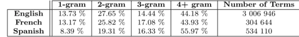
without signs. Table 4 shows the distribution in n-gram (i.e. n-gram is a term of n words, with n 1) of biomedical resources for three languages, as well as the number of terms that we took after the cleaning task. For instance, the first cell means that 13.73% of terms are composed of one word (1-gram) in UMLS for English.

1-gram 2-gram 3-gram 4+ gram Number of Terms

English 13.73 % 27.65 % 14.44 % 44.18 % 3 006 946

French 13.17 % 25.82 % 17.08 % 43.93 % 304 644

Spanish 8.39 % 19.31 % 16.33 % 55.97 % 534 110

Table 4 Details of Available Resources for Validation.

4.2 Multilingual Comparison (LabTestsOnline)

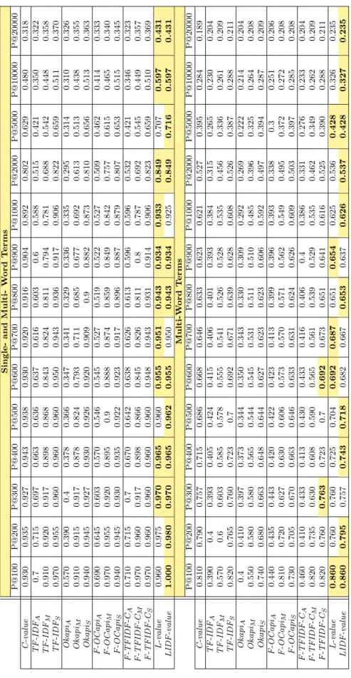
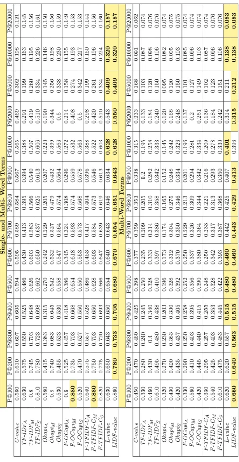
In this section, we show results obtained only with all the ranking measures, i.e. step 2 (ranking) in Figure 1. In addition, we tested the measures for single- plus multi-word terms, or just for multi-word terms in English, French and Spanish. Table 5, 6, 7 show the results in English, French and Spanish, respectively. At the top of each table, the single-word + multi-word term extraction results are presented, while the multi-word term extraction results are presented at the bottom of the table.

These tables show that LIDF-value and L-value obtain the best results for both extraction cases and for the three languages. The combined measures based on the harmonic mean, and on the SUM and MAX (i.e. F-TFIDF-CM,

F-TFIDF-CS), also give interesting results.

The single-word + multi-word term extraction results are better than just the multi-word term extraction results. The main reason for this is that the extraction of single-word terms is more efficient due to their syntactic structure (linguistic structure), i.e. usually a noun. In addition, this syntactic structure has fewer variations. The results are lower as compared to multi-word term extraction, which is more complicated and involves more variations.

We observe that LIDF-value and L-value obtain very close results. In most cases LIDF-value performs better than L-value. These two measures show that the probability associated with the linguistic patterns helps to improve the term extraction results. Note that the idf influences LIDF-value, for this reason LIDF-value has better results than L-value.

(25)

S in g le -a n d Mu lt i-W o r d T e r m s P@100 P@200 P@300 P@400 P@500 P@600 P@700 P@800 P@900 P@1000 P@2000 P@5000 P@10000 P@20000 C -v a lue 0.930 0.935 0.927 0.943 0.938 0.930 0.920 0.916 0.904 0.892 0.802 0.629 0.480 0.318 T F-I D FA 0.7 0.715 0.697 0.663 0.636 0.637 0.616 0.603 0.6 0.588 0.515 0.421 0.350 0.322 T F-I D FM 0.910 0.920 0.917 0.898 0.868 0.843 0.824 0.811 0.794 0.781 0.688 0.542 0.448 0.358 T F-I D FS 0.970 0.955 0.960 0.960 0.960 0.950 0.943 0.936 0.917 0.906 0.822 0.659 0.511 0.370 Okapi A 0.570 0.390 0.4 0.378 0.366 0.347 0.341 0.329 0.336 0.335 0.295 0.314 0.310 0.326 Okapi M 0.910 0.915 0.917 0.878 0.824 0.793 0.711 0.685 0.677 0.692 0.613 0.513 0.438 0.355 Okapi S 0.940 0.945 0.927 0.930 0.926 0.920 0.909 0.9 0.882 0.873 0.810 0.656 0.513 0.363 F-O C a p iA 0.690 0.645 0.603 0.570 0.546 0.545 0.527 0.519 0.522 0.527 0.509 0.462 0.414 0.333 F-O C a p iM 0.970 0.955 0.920 0.895 0.9 0.888 0.874 0.859 0.849 0.842 0.757 0.615 0.465 0.340 F-O C a p iS 0.940 0.945 0.930 0.935 0.922 0.923 0.917 0.896 0.887 0.879 0.807 0.653 0.515 0.345 F-T FI D F-C A 0.710 0.715 0.7 0.670 0.642 0.638 0.626 0.613 0.596 0.596 0.532 0.421 0.346 0.323 F-T FI D F-C M 0.970 0.960 0.917 0.898 0.866 0.845 0.826 0.811 0.8 0.787 0.692 0.545 0.449 0.357 F-T FI D F-C S 0.970 0.960 0.960 0.960 0.960 0.948 0.943 0.931 0.914 0.906 0.823 0.659 0.510 0.369 L -v a lue 0.960 0.975 0.970 0.965 0.960 0.955 0.951 0.943 0.934 0.933 0.849 0.707 0.597 0.431 L ID F-v a lue 1.000 0.980 0.970 0.965 0.962 0.955 0.950 0.943 0.934 0.925 0.849 0.716 0.597 0.431 Mu lt i-W o r d T e r m s P@100 P@200 P@300 P@400 P@500 P@600 P@700 P@800 P@900 P@1000 P@2000 P@5000 P@10000 P@20000 C -v a lue 0.810 0.790 0.757 0.715 0.686 0.668 0.646 0.633 0.623 0.621 0.527 0.395 0.284 0.189 T F-I D FA 0.390 0.4 0.393 0.405 0.424 0.415 0.406 0.401 0.393 0.384 0.315 0.265 0.230 0.204 T F-I D FM 0.570 0.6 0.603 0.585 0.578 0.555 0.541 0.526 0.528 0.535 0.456 0.336 0.261 0.209 T F-I D FS 0.820 0.765 0.760 0.723 0.7 0.692 0.671 0.639 0.628 0.608 0.526 0.387 0.288 0.211 Okapi A 0.4 0.410 0.397 0.373 0.344 0.350 0.343 0.330 0.309 0.292 0.269 0.222 0.214 0.204 Okapi M 0.550 0.580 0.580 0.565 0.544 0.545 0.531 0.511 0.510 0.485 0.396 0.325 0.264 0.208 Okapi S 0.740 0.680 0.663 0.648 0.644 0.627 0.623 0.623 0.606 0.592 0.497 0.394 0.287 0.209 F-O C a p iA 0.440 0.435 0.443 0.420 0.422 0.423 0.413 0.399 0.396 0.393 0.338 0.3 0.251 0.206 F-O C a p iM 0.810 0.720 0.627 0.630 0.606 0.573 0.570 0.571 0.562 0.549 0.495 0.372 0.272 0.208 F-O C a p iS 0.730 0.705 0.670 0.663 0.646 0.633 0.631 0.624 0.626 0.609 0.503 0.397 0.285 0.208 F-T FI D F-C A 0.460 0.410 0.433 0.413 0.430 0.433 0.416 0.406 0.4 0.386 0.331 0.276 0.233 0.204 F-T FI D F-C M 0.820 0.735 0.630 0.608 0.590 0.565 0.561 0.539 0.529 0.535 0.462 0.349 0.262 0.209 F-T FI D F-C S 0.820 0.760 0.763 0.723 0.7 0.692 0.673 0.651 0.641 0.616 0.525 0.390 0.288 0.211 L -v a lue 0.860 0.760 0.760 0.725 0.704 0.692 0.687 0.651 0.654 0.625 0.536 0.428 0.326 0.235 L ID F-v a lue 0.860 0.795 0.757 0.743 0.718 0.682 0.667 0.653 0.637 0.626 0.537 0.428 0.327 0.235

(26)

(27)

(28)

4.3 Evaluation of the global process (GENIA)

Since GENIA is the gold standard corpus, we conduct a detailed assessment of the experiments in this subsection. We evaluated the entire workflow of our methodology, i.e. steps 2 (ranking) and 3 (re-ranking) in Figure 1. As noted earlier, the multi-word term extraction results are influenced by the syntactic structure and their variations. So our experimentation in this subsection is focused only on multi-word term extraction.

In the following paragraphs, we also narrow down the presented results by keeping only the first 8 000 extracted terms for the graph-based measure and the first 1000 extracted terms for the web-based measure.

4.3.1 Ranking Results (step 2 in Figure 1)

Table 8 presents and compares the multi-word term extraction results with the best ranking measures, as shown earlier, i.e. C-value, F-TFIDF-CM, and

LIDF-value. The best results were obtained with LIDF-value with an11% im-provement in precision for the first hundred extracted multi-word terms. These precision results are also shown in Figure 6. The precision of LIDF-value will be further improved with TeRGraph.

C-value F -T F IDF -CM LIDF-value

P@100 0.690 0.715 0.820 P@200 0.690 0.715 0.770 P@300 0.697 0.710 0.750 P@400 0.665 0.690 0.738 P@500 0.642 0.678 0.718 P@600 0.638 0.668 0.723 P@700 0.627 0.669 0.717 P@800 0.611 0.650 0.710 P@900 0.612 0.629 0.714 P@1000 0.605 0.618 0.697 P@2000 0.570 0.557 0.662 P@5000 0.498 0.482 0.575 P@10000 0.428 0.412 0.526 P@20000 0.353 0.314 0.377

Table 8 Precision comparison of LIDF-value with baseline measures

Results of n-gram Terms

We also evaluated C-value, F-TFIDF-CM, and LIDF-value in a sequence of

n-gram terms (i.e. n-gram term is a multi-word term of n words), for this we require an index term to be a n-gram terms of length n 2. We tested the performance of LIDF-value on the n-gram term extraction taking the first 1 000 n-gram terms (n 2).

(29)

Fig. 6 Precision comparison with LIDF-value and baseline measures

Table 9 shows the precision comparison for the 2-gram, 3-gram and 4+ gram term extracted with C-value, F-TFIDF-CM, and LIDF-value. We can see

that LIDF-value obtains the best results for all intervals for any n 2. These precision results are also shown in Figure 7 for the 2-gram terms, Figure 8 for the 3-gram terms, and finally Figure 9 for the 4+ gram terms.

Table 10 shows the top-20 ranked 2-gram terms extracted with the baseline measures and LIDF-value. C-value obtained 3 irrelevant terms, F-TFIDF-C obtained 5 irrelevant terms while LIDF-value obtained only 2 irrelevant terms for the top-20 ranked 2-gram terms.

Similarly, Table 11 shows top-10 ranked 3-gram terms extracted with the baseline measures and LIDF-value. Finally, Table 12 shows the top-10 ranked 4+ gram terms extracted with the baseline measures and LIDF-value.

Note that in this context, “irrelevant” means that the terms are not in the above mentioned resources. These candidate terms might be interesting for ontology extension or population, however they must pass through polysemy detection in order to identify the possible meanings.

4.3.2 Re-ranking Results (step 3 in Figure 1)

Graph-based Results: our graph-based approach is applied to the first 8 000 terms extracted by the best ranking measure. The objective is to re-rank the 8 000 terms while trying to improve the precision by intervals. One parameter is involved in the computation of graph-based term weights, i.e. the threshold of Dice value which represents the relation when building the term graph. This involves linking terms whose Dice value of the relation is higher than threshold. We vary threshold ( ) within = [0.25, 0.35, 0.50, 0.60, 0.70] and report the precision performance for each of these values. Table 13 gives the precision performance obtained by TeRGraph and shows that it is well adapted for ATE.

(30)

2-gram terms

C-value F -T F IDF -C LIDF-value

P@100 0.770 0.760 0.830 P@200 0.755 0.755 0.805 P@300 0.710 0.743 0.790 P@400 0.695 0.725 0.768 P@500 0.692 0.736 0.752 P@600 0.683 0.733 0.763 P@700 0.670 0.714 0.757 P@800 0.669 0.703 0.749 P@900 0.654 0.692 0.749 P@1000 0.648 0.684 0.743 3-gram terms

P@100 0.670 0.530 0.820 P@200 0.590 0.450 0.795 P@300 0.577 0.430 0.777 P@400 0.560 0.425 0.755 P@500 0.548 0.398 0.744 P@600 0.520 0.378 0.720 P@700 0.499 0.370 0.706 P@800 0.488 0.379 0.691 P@900 0.482 0.399 0.667 P@1000 0.475 0.401 0.660 4+ gram terms

P@100 0.510 0.370 0.640 P@200 0.455 0.330 0.520 P@300 0.387 0.273 0.477 P@400 0.393 0.270 0.463 P@500 0.378 0.266 0.418 P@600 0.348 0.253 0.419 P@700 0.346 0.249 0.390 P@800 0.323 0.248 0.395 P@900 0.323 0.240 0.364 P@1000 0.312 0.232 0.354

Table 9 Precision comparison of 2-gram terms, 3-gram terms, and 4+ gram terms

(31)

Fig. 8 Precision comparison of 3-gram terms

Fig. 9 Precision comparison of 4+ gram terms

1 t cell t cell t cell

2 nf-kappa b nf-kappa b transcription factor

3 transcription factor kappa b nf-kappa b

4 gene expression b cell cell line

5 kappa b class ii b cell

6 cell line glucocorticoid receptor gene expression

7 b cell b activation * kappa b

8 peripheral blood b alpha * t lymphocyte

9 t lymphocyte reporter gene dna binding

10 nuclear factor endothelial cell i kappa *

11 protein kinase cell cycle binding site

12 class ii b lymphocyte protein kinase

13 b activation * nf kappa * glucocorticoid receptor

14 human t nf-kappab activation tumor necrosis

15 tyrosine phosphorylation u937 cell binding activity

16 dna binding mhc class * tyrosine phosphorylation

17 human immunodeficiency * c ebp* shift assay *

18 binding site il-2 promoter immunodeficiency virus

19 necrosis factor * monocytic cell signal transduction

20 mobility shift t-cell leukemia mobility shift

Table 10 Comparison of top-20 ranked 2-gram terms (irrelevant terms are italicized and marked with *).

(32)

C-value F -T F IDF -C LIDF-value 1 human immunodeficiency virus kappa b alpha * i kappa b

2 kappa b alpha * nf kappa b human immunodeficiency virus 3 tumor necrosis factor jurkat t cell electrophoretic mobility shift 4 electrophoretic mobility shift human t cell human t cell 5 nf-kappa b activation mhc class ii mobility shift assay 6 virus type 1 * cd4+ t cell kappa b alpha * 7 protein kinase c c-fos and c-jun * tumor necrosis factor 8 long terminal repeat peripheral blood monocyte nf-kappa b activation 9 nf kappa b t cell proliferation protein kinase c 10 jurkat t cell transcription factor nf-kappa * jurkat t cell

Table 11 Comparison of the top-10 ranked 3-gram terms (irrelevant terms are italicized and marked with *).

1 human immunodeficiency virus type 1 transcription factor nf-kappa b i kappa b alpha 2 human immunodeficiency virus type * expression of nf-kappa b * electrophoretic mobility shift assay 3 immunodeficiency virus type 1 * tumor necrosis factor alpha human immunodeficiency virus type * 4 activation of nf-kappa b normal human t cell human t-cell leukemia virus 5 nuclear factor kappa b primary human t cell nuclear factor kappa b 6 tumor necrosis factor alpha germline c epsilon transcription tumor necrosis factor alpha 7 human t-cell leukemia viru * gm-csf receptor alpha promoter t-cell leukemia virus type * 8 human t-cell leukemia virus type * il-2 receptor alpha chain activation of nf-kappa b 9 t-cell leukemia virus type * transcription from the gm-csf * peripheral blood t cell 10 electrophoretic mobility shift assay translocation of nf-kappa b * major histocompatibility complex class Table 12 Comparison of the top-10 ranked 4+ gram terms (irrelevant terms are italicized and marked with *).

TeRGraph 0.25 0.35 0.50 0.60 0.70 P@100 0.840 0.860 0.910 0.930 0.900 P@200 0.800 0.790 0.850 0.855 0.855 P@300 0.803 0.773 0.833 0.830 0.820 P@400 0.780 0.732 0.820 0.820 0.815 P@500 0.774 0.712 0.798 0.810 0.806 P@600 0.773 0.675 0.797 0.807 0.792 P@700 0.760 0.647 0.769 0.796 0.787 P@800 0.756 0.619 0.748 0.784 0.779 P@900 0.748 0.584 0.724 0.773 0.777 P@1000 0.751 0.578 0.720 0.766 0.769 P@2000 0.689 0.476 0.601 0.657 0.694 P@3000 0.642 0.522 0.535 0.605 0.644 P@4000 0.612 0.540 0.543 0.559 0.593 P@5000 0.574 0.546 0.544 0.554 0.562 P@6000 0.558 0.539 0.540 0.549 0.561 P@7000 0.556 0.540 0.540 0.545 0.552 P@8000 0.546 0.546 0.546 0.546 0.546

Table 13 Precision performance of TeRGraph when varying (threshold parameter for Dice)

Web-based Results: Our web-based approach is applied at the end of the process, with only the first 1 000 terms extracted during the previous linguistic, statistic and graph measures. For space reasons, we show only the results obtained with WAHI, which are higher than WebR.