HAL Id: hal-01065165
https://hal.archives-ouvertes.fr/hal-01065165
Submitted on 18 Sep 2014
HAL is a multi-disciplinary open access
archive for the deposit and dissemination of
sci-entific research documents, whether they are
pub-lished or not. The documents may come from
teaching and research institutions in France or
abroad, or from public or private research centers.
L’archive ouverte pluridisciplinaire HAL, est
destinée au dépôt et à la diffusion de documents
scientifiques de niveau recherche, publiés ou non,
émanant des établissements d’enseignement et de
recherche français ou étrangers, des laboratoires
publics ou privés.
Optimization methodologies for the power management
and sizing of a microgrid with storage
Rémy Rigo Mariani, Bruno Sareni, Xavier Roboam
To cite this version:
Rémy Rigo Mariani, Bruno Sareni, Xavier Roboam. Optimization methodologies for the power
man-agement and sizing of a microgrid with storage. Symposium de Génie Électrique 2014, Jul 2014,
Cachan, France. �hal-01065165�
SYMPOSIUM DE GENIE ELECTRIQUE(SGE’14) : EF-EPF-MGE 2014, 8-10 JUILLET 2014, ENS CACHAN, FRANCE
Optimization methodologies for the power
management and sizing of a microgrid with storage
Rémy Rigo-Mariani, Bruno Sareni, Xavier Roboam
Université de Toulouse, LAPLACE, UMR CNRS-INP-UPS, ENSEEIHT 2rue Camichel, 31071 Toulouse Cedex 07
ABSTRACT–In this paper, we investigate a design approach aiming at simultaneously integrating the power management and the sizing of a small microgrid with storage. We particularly underline the complexity of the resulting optimization problem and how it can be solved using suitable optimization methods in compliance with relevant models of the microgrid. We specifically show the reduction of the computational time allowing the microgrid simulation over long time durations in the optimization process in order to take seasonal variations into account.
Keywords — Smart grid, sizing, optimal dispatching, linear programming, dynamic programming, evolutionary algorithms, efficient global optimization, kriging interpolation.
RESUME –Dans cet article, nous nous intéressons à une démarche de conception optimale intégrant la planification des flux énergétiques et le dimensionnement des éléments d’un
micro-réseau avec stockage. Nous montrons plus
particulièrement comment l’adéquation entre les méthodes d’optimisation utilisées et le modèle du micro-réseau employé peut permettre la réduction significative des temps de calcul et la détermination d’une configuration optimale du micro-réseau, valable sur des horizons temporels intégrant les alternances saisonnières.
Mots clés — Smart grid, dimensionnement, plannification optimale,programmation linéaire, programmation dynamique, algorithmes évolutionaires, krigeage.
1. INTRODUCTION
With the development of decentralized power stations based on renewable energy sources, the distribution networks has strongly evolved to a more meshed model [1]. It can be considered as an association of various "microgrids" both consumer and producer that have to be run independently while granting the global balance between load and generation. Smarter operations now become possible with developments of energy storage technologies and evolving price policies [2]. Those operations would aim at reducing the electrical bill taking account of consumption and production forecasts as well as the different fares and possible constraints imposed by the power supplier [3].This paper deals with a microgrid devoted to a set of industrial buildings and factories with a typical subscribed power of 156 kW (Fig. 1a). It includes photovoltaic (PV) production and a storage unit composed of high speed flywheels(FW). The strategy chosen to manage the overall system is based on a daily off-line optimal scheduling of power flows for the day ahead. Then, in real time, an on-lineprocedure
adapts the same power flows in order to correct errors between forecasts and actual measurements [4]. Such control strategy based on the on-line adaptation of off-line optimal references has been extensively studied in the literature (e.g. [5-7] and is not the subject of this work. Our study mainly focuses on the microgrid design investigating the coupling between the power management (i.e. off-line control) and the sizing of the microgrid components (i.e. PV production and storage). Consequently, finding an optimal configuration of the microgrid results in a two level optimization problem including the optimal sizing of the microgrid and the optimal power flow dispatching over a long period of time. In the following sections, we will address this issue and its complexity with regard to energy cost optimization and computational time. To face this problem, we will show how it can be solved using suitable optimization methods in compliance with relevant models of the microgrid.
The rest of the paper is organized as follows: in the second section, the power flow model of the microgrid is presented. In section 3, several power dispatching strategies ensuring the minimization of the energy cost are compared. In particular, a fast optimization approach based on Linear Programming (LP) and on a linear model of the microgrid is introduced in order to reduce the computational time of the power flow dispatching. In section 3, a second optimization level is presented. It consists in determining the optimal sizing of the microgrid with regard to the energy cost computed over a complete year in order to take seasonal variations into account. Finally, conclusions are drawn in section 4.
2. MODEL OF THE MICROGRID
2.1. Power Flow Model of the Microgrid
The power flow model of the microgrid is given in Fig. 1b. All the microgrid components are connected though a common DC bus. Voltages and currents are not represented and only active power flows are considered.In the rest of the paper the instantaneous values are denoted as Pi(t) while the profiles over
the periods of simulation are written in vectors Pi. Due to the grid policy, three constraints have to be fulfilled at each time step t:
P1(t) 0: the power flowing through the consumption
meter is strictly mono-directional
P10(t) 0: the power flowing through the production
P6(t) 0: to avoid illegal use of the storage: flywheels
cannot discharge themselves through the production meter
A particular attention is paid to the grid power Pgrid(t)
which should comply with requirements possibly set by the power supplier: ) ( ) ( ) (t P1 t P11 t Pgrid (1) ) ( ) ( ) ( _max min _ t P t P t
Pgrid grid grid (2)
The equations between all power flows are generated using the graph theory and the incidence matrix[8]. As illustrated in Fig. 1b, three degrees of freedom are required to manage the whole system knowing production and consumption:
P5(t) Pst(t): the power flowing from/to the storage unit
(defined as positive for discharge power)
P6(t): the power flowing from the PV arrays to the
common DC bus
P9(t) ΔPPVdenotes the possibility to decrease the PVproduction (MPPT degradation) in order to fulfill grid constraints, in particular when the power supplier does not allow (or limits) the injection of the PV production into the main grid (P9is normally set to zero).
Fig.1 Studied Microgrid (a) 3D view of the factory (b) Power flow model
2.2. Efficiencies of the microgrid components
A first model (qualified as “fine model”) is defined taking account of efficiencies of power converters (typically 98 %) and storage losses. These losses are computed versus the state of charge SOC (in %) and the power Pst using a function Ploss(SOC) and calculating the efficiency with a fourth degree
polynomial FS(Pst) (see (3)). Both Ploss and FS functions are
extracted from measurements provided by the manufacturer (Levisys). Another coefficient KFS (in kW) is also introduced
to estimate the self-discharge of the flywheels when they are not used (see (4)). Once the overall efficiency is computed, the true power PFSassociated with the flywheel is calculated as
well as the SOC evolution using the maximum stored energy
EFS (here 100 kWh), the time step Δt (typically 1 hour for the
off-line optimization) and the control reference P5.
( )
( )
( )
) ( 0 ) ( ) ( ) ( ) ( ) ( 0 ) ( 5 5 5 5 5 5 t P /η t P t SOC P t P t P t P η t P t SOC P t P t P FS loss FS FS loss FS (3) 100 ) ( ) ( 0 ) ( 100 ) ( ) ( ) ( 0 ) ( 5 5 FS FS FS FS E t K t SOC t t SOC t P E t t P t SOC t t SOC t P (4)Due to the bidirectional characteristics of static converters and especially with flywheel efficiency, the overall system is intrinsically nonlinear and suitable methods have to be used to solve the optimal power dispatching problem.
3. POWER FLOW OPTIMIZATION IN THE MICROGRID
3.1. Optimal power dispatching based on the fine model
The power dispatching strategy aims at minimizing the electrical bill for the day ahead. Prices of purchased and sold energy are assumed to be time dependent with instantaneous values respectively denoted as Cp(t) and Cs(t). The time
scheduling period is one day discretized on a one hour basis within which the variables are considered to be constant. References of the power flows associated with the degrees of freedom over this period are computed in a vector
Pref=[P5 P6 P9] of 72 elements (i.e. the total number of unknowns in the corresponding optimization problem). An additional constraint is considered ensuring the same storage level SOC = 50% at the beginning and at the end of the scheduling period.Once Pref is determined, all the other power flows are computed from the forecasted values of consumption and production. Then P1 andP11 are known to estimate the balance between purchase and sale. Thus, the energy cost function is calculated as follows on the time scheduling period:
h 24 0 11 1( ). ( ) ( ). ( ) ) ( t s p t P t C t C t P C Pref (5)Due the nonlinear relations in the fine microgrid model, only nonlinear optimization methods under constraints can be used for solving the power flow problem. We remind that those methods have to take account of possible constraints on the main grid in addition to the energy cost minimization. For solving such problem several approaches have been proposed in earlier works [4], [9], [10]: Consumption Meter Production Meter Storage Degradation of the PV production DC Bus Degrees of freedom Loads PV P PPV P1 P2 P3 P4 P5 P6 P7 P8 P9 P10 P11 grid P Pload st P Photovoltaïc arrays Flywheel storage (a) (b)
Classical nonlinear programming methods and especially the trust region algorithm (TR) [11].
Stochastic optimization methods like particle swarm optimization (PSO) [12] or evolutionary approaches, especially the clearing algorithm (CL) [13] which has been shown to be highly effective for solving multimodal optimization problem because of its capacity of maintaining Darwinian evolution through a niching mechanism.
Dynamic Programming (DP) [14] which consists in a step by step minimization of the energy with regard to the storage state of charge (SOC) levels on the overall range (i.e. [0%-100%] with a given accuracy SOC. In
particular, a self-adaptive version has been developed in [9] with the aim of improving the compromise in terms of solution accuracy and computational cost.
These methods have been evaluated on a particular day whose characteristics are given in Fig. 2. The consumption profile is extracted from data provided by the microgrid owner while the production estimation is based on solar radiation forecasts computed with a model of PV arrays [15]. Energy prices result from one of the fares proposed by the French main power supplier [16] increased by 30%. Thus, the purchase costCp has night and daily values with 0.10 €/kWh from 10
p.m. to 6 a.m. and 0.17 €/kWh otherwise. Cs is set to 0.1 €/kWh
which corresponds to the price for such PV plants. In a situation with no storage device, all the production is sold (66.0 €) while all loads are supplied through the consumption meter (94.5 €). In that case, this leads to an overall cost equal to 28.5 € (Fig. 3) for the considered day. It should also be noted that no grid constraints are introduced in the investigated simulations. The initial configuration of the microgrid with 156 kW subscribed power is composed of a PV generator with a peak power of 175 kW anda 100 kW/100 kWh flywheel storage. We display in Table 1 the energy cost obtained with all dispatching methods on the initial microgrid configuration and on the particular test day. The corresponding CPU time required for obtaining the optimal solution is also mentioned in this table. Results show that the solution with minimum energy cost (indicated in bold type in Table 1) is obtained from the standard DP with an accurate discretization of the SOC level
(SOC =1%). However, the corresponding CPU time of 2 h is
quite expensive. The self-adaptive DP developed in [9] leads to a better compromise in terms of accuracy/computational cost by converging close to the optimal solution while significantly reducing the CPU time. In spite of this reduction, the computational cost of this method remains relatively important if we need to assess the energy cost over a complete year in order to take seasonal features into account. In that case, the CPU time related to the 365 successive dispatching steps will reach 10 min 365 3 days. In the context of the microgrid design where a second optimization loop is added for sizing the microgrid components, the CPU time will become prohibitive. Indeed, if 1000 microgrid simulations over one year are required for obtaining the optimal microgrid sizing, the CPU time will increase to 1000 3 days 8 years!!!. Consequently, the use of nonlinear optimization methods with the “fine” microgrid model is not suitable in the context of a design
approach integrating the microgrid sizing over long periods of time.
3.2. Fast power dispatching based on a coarse linear model
of the microgrid
In order to speed up the computational time required for the power flow dispatching in the microgrid, a fast optimization procedure has been proposed in [10]. This procedure uses LP techniques [17] on a coarse linear model of the microgrid. In this model, converter efficiencies as well as the nonlinear losses in the flywheel storage are neglected. This leads to the following simplifications: ) ( ) ( ) ( ) ( ) ( ) ( ) ( ) ( 11 10 8 7 5 4 3 2 t P t P t P t P t P t P t P t P (6) 100 ) ( ) ( ) ( 5 FS E t t P t SOC t t SOC (7)
The use of this linear model allows the formulation of the power flow dispatching problem into a linear form.
C .P
AP B ] P P P [ P L ref ref* P * 9 * 6 * 5 * ref ref arg min with . (8)
where
T
s T p T s T p L T s PV T p load ref ref L C C C C C C P C P P P C with ) ( C (9)
h 24 0 9 6 5 ) ( . ) ( ) ( . ) ( ) ( . ) ( ) ( ) ( . ) ( ) ( . ) ( ) ( t s load p PV s p s p t C t P t C t P t C t P t C t C t P t C t P C Pref (10)The constraint matrix A and vector B are built by concatenating matrices used to express each grid requirement or storage specified limits (see [10] for more details). Such problem can easily be solved using a standard LP algorithm, e.g. the Matlab© function linprogwith sparse matrices.
Fig.2 Typical test day with forecasted consumption (a) and production (b) Table 1. Comparison of power flow dispatching strategies on the test day
Power dispatching strategy Optimal cost CPU time
TR (with 50 random initial points) 1.1 € 50 min
CL (100 individuals, 50 000 generations) 0.7 € 4 h
PSO (100 particles, 50°000 iterations) 7 € 2 h
Standard DP with SOC= 10 % 3.7 € 2 min
Standard DP with SOC= 1 % 0.1 € 2 h
Self-adaptive DP 0.2 € 10 min 0 6 12 18 24 0 15 30 45 Time (h) P (k W ) a) 0 6 12 18 24 0 40 80 120 Time (h) P (k W ) b) € 66 ) ( ). ( 24 0 h t prod stP t C € 5 . 94 ) ( ). ( 24 0 h t load pt P t C
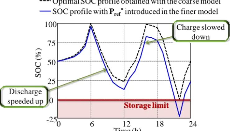
However, one drawback of this approach resides in the fact that the optimal solution found with the LP does not obviously comply with the requirements of the fine microgrid model. Fig. 3illustrates a case for which the solution Pref* obtained with LP is simulated with fine model equations. It should be noted that a deep discharge occurs at around 22 p.m. The SOC goes down to 25 % with the fine model while it remains to 0 % and fulfills the constraints with the coarse linear model. Taking account of the flywheel losses also leads to slow down the storage charge and to speed up the storage discharge.
Fig.3 Example of SOC constraint violation with the fine model using the LP optimal solution.
In the same way, the cost function returned by the coarse model is not correct. Therefore, the control references (Pref_LP) relative to the degrees of freedom obtained with the LP in association with the coarse model should be adapted in order to comply with the fine microgrid model. This can be performed using a step by step correction which aims at minimizing the cost while aligning the SOCcomputed from the fine model with the one resulting from the LP optimization (denoted as SOCLP).
At each time step t, the correction procedure is formulated as follows to find the instantaneous optimal references Pi*(t):
) ( ) ( and 0 ) ( with ) ( min arg )] ( ) ( ) ( ) ( ) ( * 9 * 6 * 5 * t t SOC t t SOC t P t P C t P t P t P t P LP * ref ref t P ref ref t nl c [ (11)where the ctnl constraint vector includes all the constraints mentioned in section 2.1. in addition to SOC and power limits.
This local minimization problem is solved using the TR method with a starting point equal to Pref_LP(t). The
convergence is ensured in all cases in a very short CPU time due to its small dimensionality (only three decision variables have to be determined, the P5 decision variable being directly
coupled with the SOC trajectory). Typically, the CPU time related to this correction procedure is less than one second over a day of simulation. The LP algorithm coupled with the coarse linear microgrid model in association with the previous correction procedure using the fine microgrid model is denoted as LPC in the following parts. This original dispatching
approach allows the reduction of the CPU time to 2 s compared with 10 min required by the self-adaptive DP to find the optimal power flow references.
We finally illustrate in Fig. 4the optimal SOC and the P1
flowprofiles obtained with the self-adaptive DP and LPC on the
particular day of Fig 2. As can be seen in Fig. 4a, both algorithms try to minimize the cost by lowering as much as possible the power flowing though the consumption meter when the energy prices remain high. The SOC profiles found by both algorithms have similar overall shapes. At the beginning of the day, the flywheel feeds the load in order to reduce the energy consumption issued from the grid. During the day, the PV production is mostly exploited to feed the load and charge the storage. The surplus is sold to generate additional benefit and no production is wasted (P9(t) 0 t) as
the injected power flowing through the main grid is not limited here. When solar radiation falls down at 8 p.m., the storage is strongly discharged until the price becomes lower at 10 p.m. The storage SOC returns to its initial state of 50 % at the end of the day so as to fulfil the requirements. As previously underlined, both solutions obtained with the self-adaptive DP and LPC are quite similar with respect to the overall cost.
However, as shown in Fig. 4c-d, the values of decision variables appear to be different. This can be explained by the non-uniqueness of the dispatching problem solutions. Indeed, this problem could be considered as an optimal energy balance between purchase, sale, storage charge or discharge. At a given time step and over a period of several hours, different power profiles can led to the same result with regard to the storage energy variations.
4. OPTIMAL DESIGN OF THE MICROGRID COMPONENTS
Due to the significant reduction of the computational cost of the power flow dispatching, the microgrid can be now rapidly simulated over long periods of time (typically one year). This allows us to study a global design approach integrating two optimization levels: power management and sizing with regard to the microgrid environment (load profiles, solar irradiation cycles). This approach is illustrated in Fig. 5. In particular, we investigate the analysis and the optimization of the microgrid with regard to several design variables:
Fig.4 Results obtained with LPC and self-adaptive DP on the particular test
day of Fig. 2. - a) P1 - b) SOC - c) P5 d) P6.
Optimal SOC profile obtained with the coarse model
0 6 12 18 24 -25 0 25 50 75 100 SO C (% ) Time (h) Discharge
speeded up Storage limit
SOC profile with Pref*introduced in the finer model
Charge slowed down 0 6 12 18 24 0 20 40 60 80 Time (h) P1 (k W ) 0 6 12 18 24 0 25 50 75 100 Time (h) S O C ( % )
Solution obtained with LPC Solution obtained with self-adaptive DP
a) b)
PV charging Consumption limited
when prices are high
c) d) 0 6 12 18 24 -60 -30 0 30 Time (h) P5 (k W ) 0 6 12 18 24 0 25 50 75 100 Time (h) P6 (k W )
Fig.5 Design approach of the microgrid integrating two optimization levels : sizing and power management
variables related to the power management of the microgrid such as the scheduling periodTschedule or the
initial SOC0 level which has to be the same at the
beginning and at the end of the scheduling period.
variables related to the microgrid sizing such as the maximum power PPV_max of the PV generator, the
maximum stored energy EFW in the flywheels and also
the subscribed power Ps to the main supplier.
4.1. Sensitivity analysis of the design variables
In this section, we first analyze the sensitivity of the design variables on the microgrid energy cost. For the 5 design variables previously mentioned, we arbitrarily define the following bounds:
0 kWh < EFW < 1500 kWh
0 kW < PPV_max < 500 kW
100 kW < Ps < 250 kW (12)
1 day < Tschedule < 120 days
0 % < SOC0 < 100 %
Several configurations of the microgrid are investigated by considering one year of simulations (i.e. 365 successive scheduling periods if Tschedule = 1 day).It should be noted that
the computational time of the power flow scheduling strongly increases when the scheduling period increases (because of the increase of the number of decision variables in the LP problem). Additional cost penalties are introduced in the cost function when the power extracted from the grid is higher than the subscribed power (i.e. Covershoot = 14 € per hour). A
sensitivity analysis is performed using a full factorial experiment [18]. The weight coefficients of the main effects (ai) of the variables and their interactions (bi) are studied as for
the following example with a two parameter function
y = f(x1,x2) modeled as follows: 2 1 1 2 2 1 1 . ˆ a x a x b x x y y (13)
In (13), ŷ is the average value of the function with the different pointsyi given by the design of experiments when the
values are at their higher (+1) or lower (1) bounds. The weight ai and bi are then computed using the columns of the
Table 2 and N the number of experiments (i.e. 4 in a problem with two parameters):
N b N a i i / / .y b .y a T i T i (14)
Table2. Full factorial design of experiments
a1=x1 a2=x2 b1=x2 x1 Y
+1 +1 +1 y1
+1 -1 -1 y2
-1 +1 -1 y3
-1 -1 +1 y4
For five design variables as for the studied case, the absolute values of the coefficients are plotted in Fig 6. The corresponding parameters (effect/interactions) are underlined. The coefficients referring to the values of EFW andPPV_max
appear to be the most influent. In a first approximation, only those variables are considered when studying different sizing cases.
4.2. Optimization of the microgrid with regard to the most influent sizing variables
We finally investigate the optimization of the microgrid with regard to the 2 most influent variables, i.e. EFW andPPV_max. The
scheduling period is set to 1 day and the initial SOC storage to 50% in all cases. Even if the CPU time devoted to the power flow dispatching has been strongly reduced with the LPc
strategy, it approximately requires 2 s 365 15 min for simulating a microgrid configuration on a complete year. This computational cost can be still view as expensive in the context of the second optimization level devoted to the microgrid sizing. In such case, the use of optimization methods based on the cost function interpolation is recommended in order to reduce the number of energy cost function calls. Among those methods, the Efficient Global Optimization algorithm (EGO) [19] is considered as one of the most effective. This algorithm estimates the cost function in unexplored points by interpolating it with the kriging method [20]. Starting from randomly chosen initial test points, the EGO investigates the search space by iteratively maximizing the Expecting Improvement (EI). This criterion expresses a compromise between the unexplored regions of the search space and the areas where the cost function appears to be the most interesting (i.e. with the lowest values). The maximization of this criterion during iterations ensures a good balance beetwen exploration and exploitation. The algorithm stops when a stoping criteria is met (e.g. fixed number of iterations, no improvement on the objective function or minimum prescribed value of the EI).All characteritics of the EGO are summurized in Fig. 7.
Fig.6. Sensitivity analysis of the design variables (a) factor effects (b) interactions effects
Optimal power dispatching (1 year)
Sizing loop
Environment: electricity rates, load
power, solar irradiation
Sizing: PV surface, storage sizing
subscribed power
Architecture : Microgrid model Power Management: Scheduling
period 0 2.104 4.104 PPV_max Ps EFW Tschedule SOC0 0 2.104 4.104 PPV_max.Tschedule PPV_max.SOC0 EFW. Ps EFW.Tschedule EFW. SOC0 Ps.Tschedule Ps. SOC0 SOC0.Tschedule PPV_max.EFW PPV_max.Ps | ai | | bi | b) a)
(b)
Fig.7. Principle of the EGO algorithm (a) synoptic (b) illustration of the EI improvement during iterations on a simple one dimensional function
The EGO is used for optimizing the microgrid with respect to the EFW and PPV_maxdesign variables. Optimizations are
performed under two different scenarios of energy price policies. In the first scenario, the electricity is sold at a high price (Cs = 10 c€/kWh) and Cp is moderate equals to
10 c€/kWh from 10 p.m. to 6 a.m. and 18 c€/kWh otherwise. In the second scenario, the purchasedcost is increased
(Cp = 16 c€/kWh from 10 p.m. to 6 a.m. and 26 c€/kWh
otherwise) and selling the PV production is not subsidized. The cost of the annual subscribed power is set to 35.3 €/kW.In addition to those operational costs computed over 365 successive days with different data related to forecast consumption and solar irradiations, we also consider the investment costs of PV generators and flywheels over 20 years of life which are respectively of 2000 €/kW and 1500 €/kWh. The microgrid Total Cost of Ownership (TCO) is then defined as the sum of the annual operational energy cost with the corresponding investment costs. This criterion is used as objective function in the EGO algorithm. The search space of the design variablesis characterized by the following bounds:
kW 500 0PPV_max (15) kWh 500 0EFW (16)
The EGO uses 10 randomly chosen starting points with a Latin Hypercube Sampling (LHS). EI is maximised using alternatively a TR method with several starting points (typically 300 points) or by regularly sampling the search space
with given steps (typically 25 kW 25 kWh). Results obtained under the two investigated scenarios are given in Table 3. In this table, we compare the optimal solution obtained from the EGO with an initial configuration of the microgrid corresponding to a situation without storage and PV production for which all the consumed energy is purchased from the main grid.Table 2 shows that EGO converges in the first scenarioto an optimal point with no storage and with a maximum number of PV panels in order to generate a maximum of profit.In the second scenario with higher energy costs and no remuneration of the PV production, adding a storage device becomes interesting with an optimum value at 44 kWh. In the same time the PV capacity is moderate at 282 kW and the self- consumption as well as the storage management allow decreasing the annual electric bill by 13 %.We illustrate in Fig. 8 the convergence of the EGO under the second scenario. It can be seen that the algorithm quickly converges to the optimal solution in a small number of iterations. The total number of cost function calls is only of 40 leading to a global CPU time close to 10 h.
5. CONCLUSIONS
In this paper, a global and integrated design approach for the power management and sizing of a microgrid with storage has been presented. The studied microgrid is composed of commercial buildings and factories with a typical subscribed power of 156 kW and includes PV production and flywheel storage. In a first part of the paper, several power flow dispatching strategies based on nonlinear optimization techniques (in particular classical nonlinear programming methods, stochastic algorithms and dynamic programming) and applied to a nonlinear model of the microgrid have been analyzed and compared with regard to their performance in terms of energy cost minimization and computational time.
Table 3. Results obtained with the EGO algorithm under the two studied scenarios: design variables and corresponding annual costs.
First scenario Second scenario
PV panel size (PPV_max) 500 kW 282 kW
Flywheel storage size (EFW) 0 kWh 44 kWh
TCO - initial configuration (k€) 97 149.3
TCO - optimal EGO solution (k€) 90 130
PV cost (k€) 50 28.1
FW cost (k€) 0 3.3
Purchased energy (k€) 64.1 98.6
Sold energy (k€) 24.2 0
Fig.8. Illustration of the EGO convergence with the second scenario
0 100 200300 400500 0 100 200 300 400 500 120 130 140 150 160 170 EVI(kWh) PPV(kWc) Co û t (k €) Starting points Optimum New points Starting Points Maximization of the EI New point (PPV, EFW) Stoping Critria ? STOP a) b) Genetic algortihm Quadratic programming Enumeration …
New point insertion
0 2 4 6 8 10 -40 -20 20 0 2 4 6 8 10 0 0.025 0.05 0 0 2 4 6 8 10 -40 -20 0 20 0 2 4 6 8 10 0 0.005 0.01 0 2 4 6 8 10 -40 -20 0 20 0 2 4 6 8 10 0 1.5. 10-3 3.10-3 0 2 4 6 8 10 -40 -20 0 20 0 2 4 6 8 10 0 3.10-5 6.10-5 EI EI EI EI Y Y Y Y X X X X X X X X Points initiaux Max EI Pour X=9.4 (Exploitation) Max EI Pour X=9.5 (Exploitation) Max EI Pour X=3.7 (Exploration) Point rajouté Itération 0 Itération 1 Itération 2 Itération 3
Interpolation with error predictor
real f unction Initial point Point insertion Max EI f or X = 9.4 Exploitation Max EI f or X = 9.5 Exploitation Max EI f or X = 3.7 Exploration Iteration 0 Iteration 1 Iteration 2 Iteration 3 0 100 200300 400500 0 100 200 300 400 500 120 130 140 150 160 170 EVI(kWh) PPV(kWc) Co û t (k €) Starting points Optimum New points Starting Points Maximization of the EI New point (PPV, EFW) Stoping Critria ? STOP a) b) Genetic algortihm Quadratic programming Enumeration … T CO (i n k €)
All of those methods can be used for predicting the day ahead the optimal references of the power flows related to the microgrid power management (especially the storage management and the exploitation of the photovoltaic production) but are too expensive in the case of the microgrid simulation over a long period of time (typically on year). Such simulations are required in the context on a second optimization step related to the microgrid component sizing taking seasonal variations into account. To face this problem an original fast power flow dispatching approach has been presented. This approach relies on the use of LP techniques in association with a coarse linear model of the microgrid in order to speed up the computational time. Then, a correction procedure is applied for aligning the results of the coarse model with that on the finer nonlinear model. This approach has shown to be highly effective leading to a significant reduction of the computational time of the power flow scheduling. In a second part of the paper, a second optimization level has been introduced aiming at finding the optimal microgrid configuration with regard to different design variables (power management variables and sizing variables). Finally the microgrid sizing has been investigated by optimizing the most influent design variables issued from a sensitivity analysis. For solving this particular problem where the objective function is still quite expensive (15 min) the EGO has been used in find the optimal microgrid configuration with a small number of objective function calls. We have voluntary restricted the study to the most important sizing variables (i.e. the PV generator and storage sizes) for simplifying the problem and for better illustrating the approach based on the use of the EGO. However, without loss of generality, this global integrated design approach could be applied with regard to additional parameters mentioned in the paper (e.g. subscribed power or scheduling period) and other scenarios of energy price policies.
6. ACKNOWLEDGMENT
This study has been carried out in the framework of the SMART ZAE national project supported by ADEME (Agence de l'Environnementet de la Maîtrise de l'Energie). The authors thank the project leader INEO-SCLE-SFE and partners LEVISYS and CIRTEM.
7. REFERENCES
[1] G. Celli, F. Pilo, G. Pisano, V. Allegranza, R. Cicoria and A. Iaria, Meshed vs. radial MV distribution network in presence of large amount of DG, Power Systems Conference and Exposition, IEEE PES, 2004. [2] S. Yeleti and F. Yong, “Impacts of energy storage on the future power
system”, North American Power Symposium (NAPS), pp. 1–7, 2010. [3] C.M. Colson, “A Review of Challenges to Real-Time Power
Management of Microgrids”, IEEE Power & Energy Society General
Meeting, pp. 1–8, 2009.
[4] R. Rigo-Mariani, B. Sareni, X. Roboam, S. Astier,.J.G. Steinmetz and E. Cahuet, “Off-line and On-line Power Dispatching Strategies for a Grid
Connected Commercial Building with Storage Unit”, 8th IFAC Power
Plant and Power System Control, Toulouse, France, 2012.
[5] H. Kanchev, D. Lu, F. Colas, V. Lazarov, and B. Francois, “Energy Management and Operational Planning of aMicrogrid With a PV-Based Active Generatorfor Smart Grid Applications”, IEEE Transactions on
Industrial Electronics, Vol. 6, pp. 45834592, 2011.
[6] M. Korpaas, A.T. Holen et R.Hildrum, “Operation and sizing of energy storage for wind power plants in a market system”, Electrical Power and
Energy Systems, Vol 25, pp 599606, 2003.
[7] T. Malakar, S.K. Goswami et A.K. Sinha, “Optimum scheduling of micro grid connected wind-pumped storage hydro plant in a frequency based pricing environment”, Electrical Power and Energy Systems, Vol 54, pp 341–351, 2014.
[8] S. Bolognani, G. Cavraro, F. Cerruti and A. Costabeber, “A linear dynamic model for microgrid voltages in presence of distributed generations”, IEEE First International Workshop on Smart Grid
Modeling and Simulation (SGMS), pp. 31-36, 2011.
[9] R. Rigo-Mariani, B. Sareni, X. Roboam and S. Astier, “Comparison of optimization strategies for power dispatching in smart microgrids with
storage”, 12th Workshop on Optimization and Inverse Problems in
Electromagnetism, Ghent, Belgium, 2012.
[10] R. Rigo-Mariani, B. Sareni, X. Roboam, “A fast optimization strategy
for power dispatching in a microgrid with storage”, 39th annual
conference of the IEEE Industrial Electronics Societey(IECON’2013), Vienna, Austria, 2013.
[11] T.F. Coleman, Y. Li, “An Interior Trust Region Approach for Nonlinear Minimization Subject to Bounds”, SIAM Journal on Optimization, Vol. 6, pp. 418–445, 1996.
[12] R.C. Eberhart and J. Kennedy, “A new optimizer using particle swarm theory”,Proceedings of the Sixth International Symposium on
Micromachine and Human Science, Nagoya, Japan. pp. 39-43, 1995.
[13] A. Pétrowski, “A clearing procedure as a niching method for genetic algorithms” in Proc. 1996 IEEE Int. Conf. Evolutionary Computation, Nagoya, Japan, pp. 798–803, 1996.
[14] P. Bertsekas, Dynamic programming and optimal control, 2nd Edition, Athena Scientific, 2000.
[15] C. Darras, S. Sailler, C. Thibault, M. Muselli, P. Poggi, J.C Hoguet, S. Melsco, E. Pinton, S. Grehant, F. Gailly, C. Turpin, S. Astier and G. Fontès, “Sizing of photovoltaic system coupled with hydrogen/oxygen storage based on the ORIENTE model”, International Journal of
Hydrogen Energy, Vol. 35, N°8, pp. 3322-3332, 2010.
[16] http://france.edf.com
[17] S.S. Rao, Engineering Optimization : Theory and Practice, John Wiley and Sons, 3rd edition, 1996.
[18] G. Taguchi, S. Chowdhury, and Y. Wu, Taguchi's Quality Engineering
Handbook, John Wiley and Sons, NJ, 2005.
[19] D.R. Jones, M Schonlau,W.J. Welch, “Efficient Global Optimization of Expensive Black-Box Functions”, Journal of Global Optimization, Vol. 13, pp. 455–492, 1998.
[20] J.P.C. Kleijnen, Kriging metamodeling in simulation: a review, Discussion paper, Tilburg University, 2007.