Approximate inference : decomposition methods with applications to networks

Approximate Inference: Decomposition Methods

with Applications to Networks

by

Kyomin Jung

B.S., Seoul National University, 2003

Submitted to the Department of Mathematics

in partial fulfillment of the requirements for the degree of

DOCTOR OF PHILOSOPHY

at the

MASSACHUSETTS INSTITUTE OF TECHNOLOGY

June 2009

@Kyomin Jung, 2009. All rights reserved.

The author hereby grants to MIT permission to reproduce and to

distribute publicly paper and electronic copies of this thesis document

in whole or in part in any medium now known or hereafter created.

Author ...

Department of Mathematics

May 1, 2009

Certified by...

...

SDevavrat

Shah

Jamieson Career Development Assistant Professor of Electrical

Engineering and Computer Science

.

Thesis Supervisor

Accepted by ...

...

Michel X. Goemans

<>7

Chair~.rc Applied Mathematics Committee

A ccepted by ...

...

David Jerison

Chairman, Department Committee on Graduate Students

MASSACHUSETTS INSTUTE OF TECHNOLOGY

JUN 2 3 2009

Approximate Inference: Decomposition Methods with

Applications to Networks

by

Kyoiin Jung

Submitted to the Department of Mathematics on May 1, 2009, in partial fulfillment of the

requirements for the degree of DOCTOR OF PHILOSOPHY

Abstract

Markov random field (MRF) model provides an elegant probabilistic framework to formulate inter-dependency between a large number of random variables. In this the-sis, we present a new approximation algorithm for computing Maximum a Posteriori (MAP) and the log-partition function for arbitrary positive pair-wise MRF defined on a graph G. Our algorithm is based on decomnposition of G into appropriately cho-sen small coInmponents; then computing estimates locally in each of these comlponents and then producing a good global solution. We show that if either G excludes some finite-sized graph as its minor (e.g. planar graph) and has a constant degree bound, or G is a polynoinially growing graph, then our algorithmn produce solutions for both questions within arbitrary accuracy. The running time of the algorithm is linear on the number of nodes in G, with constant dependent on the accuracy.

We apply our algorithm for MAP computation to the problem of learning the capacity region of wireless networks. We consider wireless networks of nodes placed in some geographic area in an arbitrary manner under interference constraints. We propose a polynomial time approximate algorithm to determine whether a, given vec-tor of end-to-end rates between various source-destination pairs can be supported by the network through a combination of routing and scheduling decisions.

Lastly, we investigate the problem of computing loss probabilities of routes in a stochastic loss network, which is equivalent to computing the partition function of the corresponding MRF for the exact stationary distribution. We show that the very popular Erlang approximation provide relatively poor performance estimates, especially for loss networks in the critically loaded regime. Then we propose a novel algorithm for estimating the stationary loss probabilities, which is shown to always converge, exponentially fast, to the asymptotically exact results.

Thesis Supervisor: Devavrat Shah

Title: Jamieson Career Development Assistant Professor of Electrical Engineering and Computer Science

Acknowledgments

This dissertation would not have been possible without the help and encouragement

from a number of people. I start by thanking my advisor, Prof. Devavrat Shah

who made it all possible for me to go through all the exciting researches. During

the course of my stay in MIT, I have learnt a lot from Devavrat. I have been with

him from the beginning, and his passion for research has infected me immensely in

my research. I cannot thank him enough for his support. I would like to thank

Prof. Michael Sipser and Prof. Jonathan Kelner for being the committee of this

dissertation. During my Ph.D. studies, I was fortunate to work with a number of

people. I have enjoyed collaborating with Matthew Andrews, Alexander Stolyar,

Ramakrishna Gummadi, Ramavarapu Sreenivas, Jinwoo Shin, Yingdong Lu, Mayank

Sharma, Mark Squillante, Pushmeet Kohli, Sung-soon Choi, Jeong Han Kim,

Byung-Ro Moon, Elena Grigorescu, Arnab Bhattacharyya, Sofya Raskhodnikova, and David

Woodruff. I thank them for many enlightening discussions we have had in the last

few years. I would also like to thank David Gamarnik, Santosh Vempala, Michael

Goemans, Madhu Sudan, Ronitt Rubinfeld, David Sontag, Kevin Matulef, Victor

Chen and many others for conversations which have influenced my research. My stay

at MIT and Cambridge was made pleasant by numerous friends and colleagues whom

I would like to thank: Tauhid Zaman, Srikanth Jagabathula, Shreevatsa Rajagopalan,

Lynne Dell, Yoonsuk Hyun, Sooho Oh, Hwanchul Yoo, Donghoon Suk, Ben Smolen,

Catherine Bolliet, Sangjoon Kim, Dongwoon Bae, Seohyun Choi, Jiye Lee, Sanginok

Han, Heesun Kim and many others. Finally, I thank my family who have supported

me in all my endeavors.

Contents

1 Introduction

1.1 Markov random field ... 1.2 Problems of interest ... 1.2.1 MAP assignment . . . . 1.2.2 Partition function . . . . 1.3 Examples of MRF... 1.3.1 Ising model . . . . 1.3.2 Wireless network . . . . 1.3.3 Stochastic loss network . 1.4 Main contributions of this thesis

2 Approximate Inference Algorithm

2.1 Previous work ...

2.2 Outline of our algorithm . . . . . . . . . .. 2.3 Graph classes ... . ... . . ...

2.3.1 Polynomially growing graph . . . . 2.3.2 Minor-excluded graph . . . . 2.4 Graph decomposition . . . . . . . . . . ....

2.4.1 (e, A) decomposition ... ... 2.4.2 Graph decomposition for polynomially growing graphs 2.4.3 Graph decomposition for minor-excluded graphs . . . . 2.5 Approximate MAP . .... . ...

2.5.1 Analysis of MAP: General G . . . .

17

.. .. . .. . . .. . .. . .. .

18

.

.

. . . .

.

2 1

2.5.2 Some preliminaries .... ... ... 55

2.5.3 Analysis of MAP: polynomially growing G ... . . 57

2.5.4 Analysis of MAP: Minor-excluded G ... . . . . . 58

2.5.5 Sequential MAP: tight approximation for polynomially growing G... ... ... 59

2.6 Approximate log Z ... ... .. 66

2.6.1 Algorithm ... ... .. 66

2.6.2 Analysis of Log Partition: General G ... . .. . . . .. 66

2.6.3 Some prelinminaries .. . ... ... . . ... ... 68

2.6.4 Analysis of Log Partition: Polynomially growing G .... . 71

2.6.5 Analysis of Log Partition: Minor-excluded G .. . . . . 72

2.7 An unexpected implication: existence of limit .. .. ... .. . ... 73

2.7.1 Proof of Theorem 8... ... . . . .... . ... .. 73

2.7.2 Proof of Lemmas .. . ... ... 74

2.8 Experiments ... ... 76

2.8.1 Setup 1 ... ... .. 77

2.8.2 Setup 2 . . . . . ... . . .. 80

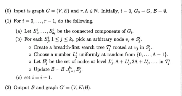
3 Application of MAP : Wireless Network 83 3.1 Capacity region of wireless network . .. . ... . ... ... 83

3.2 Previous works .... .... ... .... 84

3.3 Our contributions ... . . . ... ... ... ... . ... . 85

3.4 Model and main results .. . ... ... .. 87

3.5 Approximate MWIS for polynomially growing graphs .. . .. .. .. 89

3.6 Proof of Theorem 10 .. ... ... . 93

3.7 Algorithm ... ... ... 101

3.8 Numerical experiment ... .... ... 103

4 Application of Partition Function : Stochastic Loss Network 105 4.1 Stochastic loss network ... .. . . . . . ... 106

4.3 Our contributions ...

...

107

4.5.1 Erlang fixed-point approximation . ... 112

4.5.2 1-point approximation ... ... 113

4.5.3 Slice method ... ... .. ... .. 117

4.5.4 3-point slice method ... 118

4.6 Error in 1-point approximation ... .. 119

4.7 Error in Erlang fixed-point approximation . ... 126

4.8 Accuracy of the slice method ... .... 131

4.9 Convergence of algorithms ... ... 134

4.10 Experiments ... . .. ... 137

4.10.1 Small loss networks ... ... .. . . 138

4.10.2 Larger real-world networks ... . 140

5 Conclusion 143 5.1 Summary ... ... .. . ... ... 143

List of Figures

2-1 Vertex-decomposition for polynomially growing graphs . ... 40

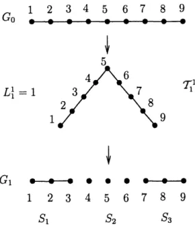
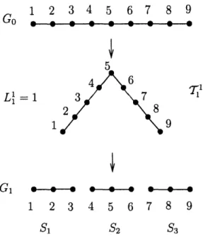
2-2 The first three iterations in the execution of POLY-V. ... . 41

2-3 Edge-decomposition for polynomially growing graphs . ... 48

2-4 Vertex-decomposition for minor-excluded graphs . ... 50

2-5 The first two iterations in execution of MINOR-V(G, 2,3). ... 51

2-6 Edge-decomposition for minor-excluded graphs . ... 52

2-7 The first two iterations in execution of MINOR-E(G, 2, 3). ... 53

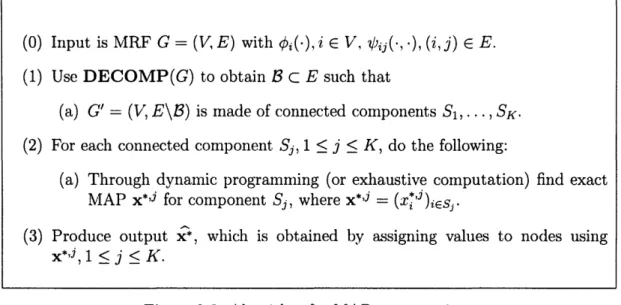
2-8 Algorithm for MAP computation . ... . . . . 54

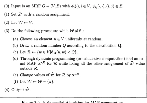
2-9 A Sequential Algorithm for MAP computation . ... 60

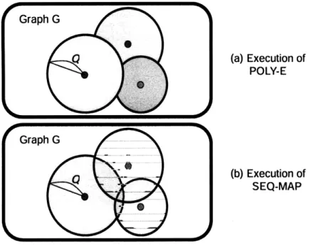
2-10 Comparison of POLY-E versus SEQ-MAP. . ... 61

2-11 Algorithm for log-partition function computation . ... 67

2-12 Example of grid graph (left) and cris-cross graph (right) with n = 4.. 76

2-13 Comparison of TRW, PDC anld our algorithm for grid graph with n = 7 with respect to error in log Z. Our algorithm outperforms TRW and is competitive with respect to PDC. . ... .. 77

2-14 The theoretically computable error bounds for log Z under our algorithm for grid with n = 100 and n = 1000 under varying interaction and varying field model. This clearly shows scalability of our algorithm. . ... . 78

2-15 The theoretically computable error bounds for MAP under our algorithm for grid with n = 100 and n = 1000 under varying interaction and varying field model ... .... ... 79

2-16 The theoretically computable error bounds for log Z under our algorithm for cris-cross with n = 100 and n = 1000 under varying interaction and varying field model. This clearly shows scalability of our algorithmn and robustness

to graph structure. . . . .... . ... . . ... .. . 80

2-17 The theoretically computable error bounds for MAP under our algorithm for cris-cross with n = 100 and n = 1000 under varying interaction and varying field model. ... . . . ... .... ... 81

3-1 Randomized algorithm for approximate MWIS .. ... . 90

3-2 Queue computations done by the algorithm .. ... ... 96

3-3 An illustration of the cyclical network with 2-hop interference. ... 103

3-4 A plot of q"nar(t) versus t on the network in Figure 3.8 for 6 different rate vectors. ... ... .. . ... . . .. . .. 104

4-1 An iterative algorithm to obtain a solution to the fixed-point equations (4.4)... ... 113

4-2 An coordinate descent algorithm for obtaining a dual optimum. .... 114

4-3 Description of the slice method ... .... . . ... .... 118

4-4 Illustration of the small canonical network model. ... ... 138

4-5 Average error of loss probabilities computed for each method as a func-tion of the scaling parameter N . ... ... . ... . . . . . . 139

List of Tables

Chapter 1

Introduction

A Markov random field (MRF) is an abstraction that utilizes graphical

represen-tation to capture inter-dependency between a large number of random variables.

MRF provides a convenient and consistent way to model context-dependent entities

such as network nodes with interference and correlated features. This is achieved by

characterizing mutual influences among such entities. The MRF based models have

been utilized successfully in the context of coding (e.g. the low density parity check

code [51]), statistical physics (e.g. the Ising model [11]), natural language

process-ing [43] and image processprocess-ing in computer vision [36,42, 64]. The key property of

this representation lies in the fact that the probability distribution over the random

variables factorizes.

The key questions of interest in most of these applications are that of inferring

the most likely, or Maximum A-Posteriori (MAP), assignment, and computing the

normalizing constant of the probability distribution, or the partition function. For

example, in coding, the transmitted message is decoded as the most likely code word

from the received message. This problem corresponds to computing MAP assignment

in an induced MRF in the context of graphical codes (aka LDPC codes). These two

problems are NP-hard in general. However, in practice, the underlying graphical

structure of MRF is not adversarial and hence can yield to simple structure aware

approximations. In this dissertation, we identify new classes of structural properties

of MRFs that yield to simple, and efficient algorithms for these problems. These

algorithms and presented in Chapter 2.

Then we present application of our algorithms to networks. In wireless network settings, in essence we have a network of n nodes where nodes are communicating over a common wireless medium using a certain standard communication protocol (e.g. IEEE 802.11 standard). Under any such protocol, transmission between a pair of nodes is successful if and only if none of the nearby or interfering nodes are trans-mitting sinmultaneously. Any such interference model is equivalent to an independent

set interference model over the graph of interfering communication links. In this

model, the well known "maximum weight scheduling" introduced by Tassiulas and Ephrenides [61] is equivalent to the computation of maximurm weight independent

set by considering each node's queue size as its weight. In Chapter 3, by

consider-ing the maximum weight independent set problem as computation of MAP for the corresponding MRF and applying our approximate MAP algorithm, we propose an algorithm for learning the capacity region of a wireless network.

Finally, in Chapter 4, we investigate the problem of computing loss probabilities of routes in a stochastic loss network, which is equivalent to computing log-partition functions of the corresponding MRF for the exact stationary distribution. For this problem, we propose a novel algorithm for estimating the stationary loss probabilities

in stochastic loss networks, and show that our algorithm always converges,

exponen-tially fast, to the asymptotically exact solutions.

1.1

Markov random field

An MRF is a probability distribution defined on an undirected graph G = (V, E) in

the following manner. For each v E V, let X, be a random variable taking values in some finite valued space E,,. Without loss of generality, assume that E, = E for all

v E V. Let X = (X1,..., X,) be collection of these random variables taking values in EC . For any subset A C V, we let XA denote {X,,v E A}. We call a subset

S C V a cut of G if by its removal from G the graph decomposes into two or more

any a E A,b E B, (a, b) 0 E.

Definition 1 The probability distribution X is called a Markov random field, if for

any cut S C V, XA and XB are conditionally independent given Xs, where V\S = AUB.

By the Hammersley-Clifford theorem [22], any positive Markov random field, i.e.

distribution over cliques of the graph. That is, let

CG

be the collection of the cliques

of G, and T, be a positive real valued potential function defined on a clique c E CG.

Then the MRF X can be represented by

P [X=x] oc

r

(x).

In Chapters 2 and Chapter 3, we will restrict our attention to pair-wise MRFs, i.e.

MRFs having the above potential functions decomposition with cliques only on the

vertices and the edges of G. This does not incur loss of generality for the following

reason. A distributional representation that decomposes in terms of distribution over

cliques can be represented through a factor graph over discrete variables. Any factor

graph over discrete variables can be transformed into a pair-wise Markov random field

(see, [66] for example) by introducing auxiliary variables. Now, we present a, precise

definition of the pair-wise Markov random field.

Definition 2 For each vertex v E V and edge (u, v) E E, let there be a corresponding

potential function

I,,

which has the following form is called a pair-wise Markov random field.

P[X=x] oc

'(X)

1-

(1.1)

vEV (u,v)EE

In Chapter 4, we will study a class of non pair-wise MRF with application to a

stochastic loss network. Its definition is explained in Section 1.3.3.

1.2

Problems of interest

In this section, we present the two most important operational questions of interest for a pair-wise MRF : computing most likely assignment of unknown variables, and computation of probability of assignment given partial observations.

1.2.1

MAP assignment

The maximum a posteriori (MAP) assignment x* is an assignment with maximal probability, i.e.

x* E arg

max

xEEr

In many inference problems, the best estimator is the Maximum Likelihood (ML) estimator. In the MRF model, this solution corresponds to a MAP assignment. Computing a MAP assignment is of interest in a wide variety of applications. In the context of error-correcting codes it corresponds to decoding the received noisy code-word, and in image processing, it can be used as the basis for image segmentation techniques. In the statistical physics applications, the MAP assignment corresponds to the ground state, or a state with minimum energy. In discrete optimization ap-plications, including computation of a maximum weight independent set, the MAP assignment corresponds to the optimal solution.

In our pair-wise MRF setup, a MAP assignment x* is defined as

1.2.2

Partition function

The normalization constant in the definition (1.1) of distribution is called the partition

function denoted by Z. Specifically,

Notice that Z is dependent on the potential function expression, which may not be

unique for the given MRF distribution (for example, by adding constants to is).

Clearly, the knowledge of Z is necessary in order to evaluate probability

distri-bution or to compute marginal probabilities, i.e. P(X, = x,) for v E V. Under the polynomial (over n) time computational power, computing Z is equivalent to

com-puting P[X = x] for any x E E".In applications in statistical physics, logarithm of Z provides free-energy, and in reversible stochastic networks, Z provides loss probability for evaluating quality of service (see Chapter 4).

1.3

Examples of MRF

In this section we provide some examples of the MRF in the statistical physics and

the network world. Some of which will be useful later in the thesis.

1.3.1

Ising model

The Ising model, introduced by Ernst Ising [20] is a mathematical model to under-stand structure of spinglass material in statistical physics [59]. In essence, the model is a binary pairwise MRF defined as follows. Let V be a collection of vertices, each corresponding to a "spin". For v E V, let X, denote its spin value in {-1, 1}. Let

E E V x V be collection of edges capturing pair-wise interaction between spins. Then

the total energy of the system for each spin configuration x E {-1, 1}Iv l is given as follows.

For x E {-1, 1}IVI,

E(x) oc - J,xx,, (1.2)

(u,v)EE

where J,, E R are constants. For each pair (u, v) E E, if J,, > 0, the interaction is called ferromagnetic. If J, < 0, then the interaction is called antiferromagnetic.

does form an pair-wise MRF defined on G := (V, E). Let the inverse temperature be

1

kBT'

where kB is the Boltzmann's constant, and T is the temperature of the system. Then the partition function of the following pair-wise MRF

Z=

E

E(13x)

xE{-1,1}"

corresponds to the thermodynamic total energy of the system [11], which allows us to calculate all the other thermodynamic properties of the system. For this MRF, the MAP assignment corresponds to the ground state, or the state with minimum energy. As an approximation model, Ising model defined on finite dimensional grid graphs, especially on 2-dimensional or 3-dimensional grid graphs are widely used. Generalized forms of Ising model which also contain potential functions for single spins, are widely used for applications in computer vision including image segmentation problems [36].

1.3.2

Wireless network

The primary purpose of a communication network is to satiate heterogeneous demands of various network users while utilizing network resources efficiently. The key algorith-mic tasks in a communication network pertain scheduling (physical layer) and conges-tion control (network layer). Recent exciting progress has led to the understanding that good algorithmic solution for joint scheduling and congestion control can be ob-tained via the "maximum weight scheduling" of Tassiulas and Ephremides [61]. In Chapter 3, we will investigate this scheduling algorithm extensively.

Consider a wireless network on n nodes defined by a directed graph G = (V, E)

with IVI = n, Ej = L. For any e E E, let a(e), f(e) denote respectively the originI

and destination vertices of the edge e. The edges denote potential wireless links, and only the subsets of the edges so that any pairs of the edges in it do not interfere can

be simultaneously active. We say two edges interfere when they share a vertex. Let

S = {e E {0, ₁}L : e is the adjacency vector for a non-interfering subset of E}

Note that S is the collection of the independent sets of E by considering interference among el E E and e2 E E as the edge between them.

Consider m distinct source destination pairs of the network, (sl, dl),..., (sn, d,,)

and an end to end rate vector, r = (r1, r2, ... , rm) E [0, 1]m.Let t be an index ranging

over integers, to be interpreted as slotted time. Define Vi(t) E R+ as the packet mass at node i destined for node dj at time t (for 1 < i < n, 1 < j < m). Define a weight

matrix at time t, W(t), of dimension L x m via its (I, j)th element (1 < 1 < L and

1 < j < M):

w'

qa(

)(t)

The weight vector of dimension L, W(t), is then defined with its Ith element

(corre-sponding to link 1, 1 < I < L) as

W(t) = max{W/ (t)}. (1.5)

Let a-b denote the standard inner product of a and b. Then let the maximum

weight independent set (MWIS) of links be

.i (t) = max e - W(t). (1.6)

eES

We will define an MRF so that computing MAP in the MRF is equivalent to

com-puting MWIS of the network. In general, given a graph G = (V, E) and node weights

given by w = (wil,...,

wiv)

maximum weight independent set x* is defined by x* = argmax (wT x: x E Z(G)

},

where we consider w as an element of {0, 1}IV.

independent set of links for each time t is throughput optimal. However, it is well

known that finding maximunm weight independent set in general graph is NP-hard [1]

and even hard to approximate within ln-O(1) factor (B/20 (v'°ogB) factor for degree B

graph) [60].

Consider a subset of V as a binary string x E {0, 1}( _{. The following pair-wise}

MRF model is widely used to design approximate solution of the maximum weight independent set (MWIS) for many class of networks, where the weight W0 of node 'v

is defined as in (1.5).

(1.7)

where I is

defined so that

T(xl,

For the above MRF, note that W4/(x) is 0 if x is not an independent set of G.

When x is an independent set of G, W(x) is proportional to the exponent of total

weight of x. Hence, computation of MAP assignment for the above MRF corresponds to computation of the MWIS. Details of this model will be discussed in Chapter 3.

1.3.3

Stochastic loss network

For almost a century, starting with the seminal work of Erlang [8], stochastic loss networks have been widely studied as models of many diverse computer and com-munication systems in which different types of resources are used to serve various classes of customers involving simultaneous resource possession and non-backlogging

workloads. Examples include telephone networks, mobile cellular systems, ATM

net-works, broadl)and telecommunication netnet-works, optical wavelength-division multi-plexing networks, wireless networks, distributed computing, database systems, data, centers, and multi-item inventory systems. see, e.g., [21,28 31,44, 45, 53, 54, 68, 69].

Loss networks have been used recently for resource planning in the IT services in-dustry, where a collection of IT service products are offered each requiring a set of resources with certain capabilities [4, 39]. In each case, the stochastic loss network

W(x)

c

exp

WH(r -x, -

(xI

xV),

is used to capture the dynamics and uncertainty of the computer/communication application being modeled.

In Chapter 4, we investigate stochastic loss networks with fixed routing, by con-sidering the Markov random field for its stationary distribution. Consider a network with J links, labeled 1, 2,..., J. Each link j has C units of capacity. There is a set of K distinct (pre-determined) routes, denoted by R =

{1,..., K}. A call on route r

j,

an independent Poisson process of rate r, with v = (v1

,...,

of these rates. The dynamics of the network are such that an arriving call on route

r is admitted to the network if sufficient capacity is available on all links used by

route r; else, the call is dropped (or lost). To simplify the exposition, we will assume that the call service times are i.i.d. exponential random variables with unit mean. It is important to note, however, that our results in this thesis are not limited to these service time assumptions since the quantities of interest remain unchanged in the stationary regime under general service time distributions due to the well-known

insensitivity property [63] of this class of stationary loss networks.

Let n(t) = (nl(t),...,nK(t)) E NK be the vector of the number of active calls in the network at time t. By definition, we have that n(t) E S(C) where

S(C) = {n E ZKjn 0,An < C ,

and C = (C1,..., Cj) denotes the vector of link capacities. Within this framework,

the network is Markov with respect to the state n(t). It has been well established that the network is a reversible multidimensional Markov process with a, product-form stationary distribution [27]. Namely, there is a unique stationary distribution 7r on

the state space S(C) such that for n E S(C),

r(i)

=

G(C)

]

(1.8)

where G(C) is the normalizing constant, or the partition function

G(C)=

.

nES(C) rER Z

-Let M be an upper bound on the number of active route calls for all routes. Then the distribution (1.8) can be understood as the following Markov random field defined for n E M'.

i(LI) 0C v" (1.9)

r'R R j=1

where Rj is the set of routes that uses link j, and gj(.) is a potential function defined as

J

if

A].ni.

gj(nR,) =

if

A

0 otherwise

The underlying graph of the above MRF is the factor graph of 7r.

Definition 3 A factor graph is a bipartite graph that expresses the factorization structure of a multivariate function as 7r defined in (1.9): 1) it has a variable node for each variable n,.; 2) it has a factor node for each local function gj; 3) there is an edge connecting variable node 71r to factor node gj if and only if nr is an argument of

gj

-For this model, a main algorithmic question of interest is computing the probability over time that a call on a route will be lost. This probability is called the loss

probability of the route. In Chapter 4, we will discuss a well known approach for

this computation called Erlang's fixed-point approximation, and its limitation. Then we will provide a novel algorithm for this problem and its comparison with Erlang's

1.4

Main contributions of this thesis

Exact computation of MAP assignment and log-partition function for an MRF on

general graph are known to be NP-hard, and sometimes they are even hard to

ap-proximate within nl-o

)

factor [1, 60]. However, applications require solving this

problem using very simple algorithms. Hence designing efficient and easily

imple-mentable approximate algorithms for those problems for practical MRFs is of main

algorithmic challenge.

One popular approach in the literature is that of the Belief Propagation algorithm

and its deviations including Tree-reweighted algorithm, which exploit large "girth"

(i.e. lack of short cycles) of the graphical structure. While these algorithms have been

successful in situations like error-correcting codes where one has "freedom" to design

the graph of code, in applications like wireless network, stochastic loss network, image

processing, and statistical physics, this is not the case. Specifically, popular graphical

models for wireless network, and image processing do have lots of short cycles.

In this thesis, we identify a new class of structural properties of MRF, that yield

to simple, and efficient algorithms. Specifically, for MRFs defined on graphs that

have some "geometry" (which we call as graphs with polynomial growth, see Section

2.3.1) or graphs which are minor-excluded (for example, planar graphs, see Section

2.3.2) with bounded degree, we design almost linear time algorithms for

approxi-mate computation of MAP assignment and log-partition function within arbitrary

accuracy. The graphical models arising in wireless networks, statistical physics, and

image processing do possess such graphical structure. We also provide a simple novel

algorithm for MAP computation based on local updates of a, MAP assignment. Our

algorithm can be implemented in a distributed manner, and we show that for graphs

with polynomial growth, our algorithm computes approximate MAP within arbitrary

accuracy. These algorithms are presented in Chapter 2. A subset of the results of

Chapter 2 appeared in [25].

Next, we turn our attention to the application of our algorithms to network

prob-lems. In Chapter 3, we consider a wireless network of n nodes placed in some

ge-ographic area in an arbitrary manner. These nodes communicate over a common wireless medium under some interference constraints. Our work is motivated by the need for an efficient algorithm to determine the n2 dimensional unicast capacity re-gion of such a wireless network. Equivalently, we consider the problem of determining whether a given vector of end-to-end rates between various source-destination pairs can be supported by the network through a combination of routing and scheduling decisions among more than exponentially many possible choices in n.

This question is known to be NP-hard and hard to even approximate within

nl-o( 1) factor for general graphs [57]. We consider wireless networks which are usually formed between nodes that are placed in a geographic area, and come endowed with a certain "geometry", and show that such situations do lead to approximations to the MWIS problem by applying our approximate computation of MAP algorithm to the corresponding MRF. Consequently, this gives us distributed polynomial time algorithm to approximate the capacity of wireless networks to arbitrary accuracy. This result hence, is in sharp contrast with previous works that provide centralized algorithms with at least a constant factor loss. Results reported in this Chapter appeared in [13,14,26].

In Chapter 4, we investigate the problem of computing loss probabilities of routes in a stochastic loss network, which is equivalent to computing partition function of the corresponding MRF for the exact stationary distribution. We show that the very popular Erlang fixed-point approximation provides relatively poor performance estimates, especially when the loss network is critically loaded. Then based on the structural property of the corresponding MRF, we propose a novel algorithm for estimating the stationary loss probabilities in stochastic loss networks, and show that our algorithm always converges exponentially fast to the asymptotically exact solutions. Using a variational characterization of the stationary distribution, we also provide an alternative proof for an error upper bound of the Erlang approximation. A previous version of this Chapter appeared in [24].

Chapter 2

Approximate Inference Algorithm

In this Chapter, we present new approximate inference algorithms for computation of MAP assignment and log-partition function for two important classes of pairwise MRFs based on the underlying graph structure of the MRF. The first class is the graphs that are polynomially growing, and the second one is the graphs that exclude a finite-sized graph as a minor and has a constant vertex degree bound. For the class of polynomially growing graph, we also provide an intuitively pleasing sequential randomized algorithm for efficient inference of MAP.

2.1

Previous work

A plausible approach for designing simple algorithms for computation of MAP and log-partition function is as follows. First, identify a wide class of graphs that have simple algorithms for computing MAP and log-partition function. Then, for any given graph, approximately compute a solution by possibly solving multiple sub-problems that have good graph structures and then combining the results from these sub-problems to obtain a, global solution.

Such an approach has resulted in many interesting recent results starting from the Belief Propagation (BP) algorithm designed for tree graphs [49]. Since there is a vast literature on this topic, we will recall only few results. Two important algorithms are the generalized belief propagation (BP) [71] and the tree-reweighted

algorithm (TRW) [65-67]. Key properties of interest for these iterative procedures are the correctness of fixed points and convergence. Many results characterizing properties of the fixed points are known starting [71]. Various sufficient conditions for their convergence are known starting [62]. However, simultaneous convergence and correctness of such algorithms are established for only specific problems, e.g. [3,34,46]. Now, we discuss two results relevant to this chapter. The first result is about prop-erties of TRW. The TRW algorithm provides proval:le upper bound on log-partition function for arbitrary graph [67]. However, to the best of our knowledge the error is not quantified. The TRW for MAP estimation has a strong connection to specific Linear Programming (LP) relaxation of the problem [66]. This was made precise in a sequence of work by Kolmogorov [33], Kolmogorov and Wainwright [34] for binary MRF. It is worth noting that LP relaxation can be poor even for simple problems.

Another work is an approximation algorithm proposed by Globerson and Jaakkola [12] to compute log-partition function using Planar graph decomnposition (PDC). PDC uses techniques of [67] in conjunction with known result about exact computation of partition function for binary MRF when G is Planar and the exponential family has very specific form. Their algorithm provides provable upper bound for arbitrary graph. However, they do not quantify the error incurred. Further, their algorithm is limited to binary MRFs.

2.2

Outline of our algorithm

We propose a novel local algorithm for approximate computation of MAP and log-partition function. For any e > 0, our algorithm can produce an E-approximnate solution for MAP and log-partition function for arbitrary positive MRF G as long as

G has either of these two properties:

* G is a polynomially growing graph (see Section 2.3.1, Theorems 2 and 6),

* G excludes a finite-sized graph as a minor (see Theorems 3 and 7) and has constant maximum degree.

We say MRF X is a positive MRF when X is given as follows: for x E E7',

P[X = x] oc exp ,(x,) (X+ E,, ;x ) (2.1)

vEV (U,V)EE

where $, : E -- R+ and

4u

being non-negative does not incur loss of generality for the following reasons: (a) the distribution remains the same if we consider potential functions 0, + C,, ,,, +

Cv, for all v E V, (u, v) E E with constants C, C,,; and (b) by selecting large enough constant, the modified functions will become non-negative as they are defined over finite discrete domain. The representation (2.1) is called a exponential family

distribution.

Our algorithm is primarily based on the following steps.

* First, decompose G into small-size connected components say G1,..., Gk by

removing few edges of G.

* Second, compute estimates (either MAP or log-partition) in each of Gi sepa-rately.

* Third, combine these estimates to produce a global estimate while taking care of the effect induced by removed edges.

In general, our algorithm works for any G and we can quantify bound on the error incurred by our algorithm. It is worth noting that our algorithm provides a provable lower bound on log-partition function as well unlike many of previous works. We show that the error in the estimate depends only on the edges removed. This error bound characterization is applicable for arbitrary graph.

For obtaining sharp error bounds, we need good graph decomposition schemes. Specifically, we use a simple and very intuitive randomized decomposition scheme for graphs with polynomial growth. This decomposition is described in Section 2.4.2. For minor-excluded graphs, we use a simple scheme based on work by Klein, Plotkin and Rao [32] and Rao [50] that they had introduced to study the gap between max-flow

and miin-cut for multicornmmodity flows. This decomposition scheme is described in Section 2.4.3. In general, as long as G allows for such good edge-set for decomposing G into small components, our algorithm will provide a good estimate.

To compute estimates in individual components, we use dynamic programming. Since each component is small, it is not computationally burdensome. However, one may obtain further simpler heuristics by replacing dynamic programming by other method such as BP or TRW for computation in the components.

The running time of our algorithms are 0(n), with the constant dependent on e and (a) growing rate for polynomially growing graph, or (b) maximum vertex degree and size of the graph that is excluded as minor for minor-excluded graphs. For example, for 2-dimensional grid graph, which has growth rate 0(1), the algorithm takes C(e)n time, where loglogC(e) = 0(1/e). On the other hand, for a planar graph with constant maximum vertex degree, the algorithm takes C'(e)n time, with log log C'(e) = 0(1/e).

In Section 2.5.5, we develop an intuitively pleasing sequential randomized algo-rithm for approximate MAP computation for polynomially growing graphs. This is motivated by the property of the decomposition scheme for that graph class. This algorithm can be implemented in a distributed manner in a natural way. We strongly believe that this algorithm will have great practical impact.

In Section 2.7, as an unexpected consequence of these algorithmic results, we obtain a method to establish existence of asymptotic limits of free energy for a class of MRF. Specifically, we show that if the MRF is d-dimensional grid, and all node, edge potential functions are identical, then the free-energy (i.e. normalized log-partition function) converges to a limit as the size of the grid grows to infinity. In general, such approach is likely to extend for any regular enough MRF for proving existence of such limit: for example, the result will immediately extend when one replaces the node, edge potential being exactly the same by they being chosen from a common distribution in an i.i.d. fashion.

Finally, in Section 2.8, we present numerical experiments which convincingly show that our algorithms are very competitive to other recently successful algorithms

in-cluding TRW and PDC.

2.3

Graph classes

In this section, we explain the two class of graphs for which we obtain approximate inference algorithms.

2.3.1

Polynomially growing graph

Definition 4 Let dG be the shortest path distance metric of a given graph G, and let

BG(v,r) = {w E VldG(w,v) < r}. If there are constants C > 0 and p > 0 so that

for any v E V and r E N,

IBc(v, r) < C - r",

then we say G is polynomially growing with growth rate p and corresponding constant

C.

Practical applications of MRF model including the following geometric network graphs and doubling dimensional graphs, satisfy the above property.

Example 1 : Geometric Graph. Consider a wireless network with n nodes rep-resented by the vertices V = {1,..., n} placed in a 2-dimensional geographic region given by the /7 x vi square of area n1 in an arbitrary manner (not necessarily random). Let E be the set of edges between nodes indicating which pair of nodes can communicate. Let dE(., -) be the Euclidean distance of the Euclidean space. Given a vertex v E V, let BE(v, r) = {u E V : dE(u, v) < r}. We assume that the wireless network satisfies the following simple assumptions.

1. There is an R > 0 such that no two nodes having distance larger than R

'Placing the nodes in the specified square is for simple presentation. The same result holds when the nodes are placed in any Euclidean rectangle, and when the nodes are place in any region of k-dimensional Euclidean space.

can establish a communication edge with each other2 _{where R is called the}

transmission radius.

2. Graph G has bounded density D > 0, i.e. for all v E V, BE(v,R)l

<

A geometric random graph obtained by placing n nodes in the V x f square uni-formly at random and connecting two nodes that are within distance R = O(Vogn)

of each other satisfies the previous assumptions with high probability.

Lemma 1 Any geometric graphs satisfying the above two assumptions are

polynomi-ally growing with growth rate 2.

Proof. Let G be a geometric graph with a transmission radius R and a bounded

density D. First, note that in the Euclidean space, for any r > R, BE(v, r) can be

covered by 6 ((_)2) many balls of radius R. Hence, together with the definition of the bounded density D, there is a constant D' > 0 so that for all v E V and r > R,

BE(,r)I

<

r2

Now, for a given two connected vertices v, w E V of G, let v = vo, v, v2 ... , ve = w

be a shortest path in G. By the definition of the transmission radius, for all i = 0, 1..., (V- 1),

dE(Vi, Vi+1) < R.

By the triangular inequality in the Euclidean metric,

dE(v, w) dE(Vi, vi+1)

<

.

i=O

So we obtain

dE(v, w) <

Re

R

Hence, for any v E V and r E N,

BG(v, r) C BE(v,

Rr).

From (2.2),

IBa(v, r)

I

<

which shows that the growth rate of G is 2.

Example 2 : Doubling Dimensional Graph. A graph is said to have a doubling

be covered by at most 2w many balls of radius r for any r E N. A graph with a

constant doubling dimension is called a doubling dimensional graph. The notion of

doubling dimensional graphs was first introduced in [2, 15, 17]. It is easy to check

that a grid graph Zd has doubling dimension d. Clearly, any graph with n nodes

has doubling dimension at most 0(log

n). The following Lemma shows that any

doubling dimensional graph is polynomially growing.

Lemma 2 A graph with a constant doubling dimension o is polynomially growing

Proof. First, we will show that for any x E V and any t E Z+,

IBc(x,

2t) I

<

2

(2.3)

The proof of (2.3) is by induction on t E Z+. For the base case, consider t = 0. Now,

BG(x, 20) is essentially the set of all points which are at distance less than 1 from

x by the definition. Since it is metric with distance being integer, this means that

BG(x, 1) =

{x}. Hence,

1)1

for all x

X.

Now suppose that the claim of Lemma is true for all t < k and all x E X. Consider

balls of radius 2k, say BG(yj, 2k) with yj E X for 1 < j

{,

<

By inductive hypothesis, for 1 < j < f,

BcG(yj, 2k)I < 2kp.

Since we have £ < 2(, we obtain

IBG(x, 2k +l ) < 2kp < 2(k+1)W

This completes the proof of inductive step, and that of (2.3).

Now, for any r E N, and any x E V, let 2t < r < 2t+1 for t E Z+. From (2.3), we

obtain that

IBG(x, r) IBG(x, 2t+1)l < 2(t+ l ) = 2 -(2t)O < 2O ~r , (2.4) which shows the Lemma.

Property of polynomially growing graphs. The following Lemma shows that any subgraph of a polynomnially growing graph is also a polynomially growing graph.

Lemma 3 If G is polynomially growing with growth rate p, any subgraph G = (V, E)

of G obtained by removing some edges and vertices of G is also polynomially growing "with growth rate at

rmost

Proof. For any vertex v, w E V, note that

since any path in G from v to w is also a path in G. Hence, for any v E V and r E N,

Be(v, r) C Bc(v, r).

Hence,

[Be(v, r) < IBG(V, r)lT < rp ,

which shows the Lemma from the definition 4. For example, any subgraph of a grid graph is a polynomially growing graph.

2.3.2

Minor-excluded graph

Next, we introduce a class of graphs known as minor-excluded graphs (see a series of publications by Roberston and Seymour under the graph minor theory project [52]). A graph H is called minor of G if we can transform G into H through an arbitrary sequence of the following two operations:

* removal of an edge.

* merge two connected vertices u, v: that is, remove edge (u, v) as well as vertices

u and v; add a new vertex and make all edges incident on this new vertex that

were incident on u or v.

Now, if H is not a minor of G then we say that G excludes H as a minor.

The explanation of the following statement may help to understand the definition better: any graph H with r nodes is a minor of K,, where Kr is a complete graph of r nodes. This is true because one may obtain H by removing edges from Kr that are absent in H. More generally, if G is a subgraph of G' and G has H as a minor, then G' has H as its minor. Let Kr,r, denote a complete bipartite graph with r nodes in each partition. Then Kr is a minor of Kr,r. Hence, any graph H with r nodes is a, minor of Kr,r. An important implication of this is as follows: to prove property P for graph G that excludes H, of size r, as a minor, it is sufficient to prove that any graph that excludes Kr,r as a minor has property P. This fact was cleverly used by

Klein et. al. [32]. In what follows and the rest of the paper, we will always assume r to be some finite number that does not scale with n (the number of nodes in G).

2.4

Graph decomposition

In this section, we introduce notion of our graph decomposition. We describe very simple algorithms for obtaining decomposition for graphs with polynomial growth and minor-excluded graphs.

2.4.1

(e,

A) decomposition

Given , A > 0, we define notion of (e, A) decomposition for a graph G = (V, E).

This notion can be stated in terms of vertex-based decomposition or edge-based de-composition.

Definition 5 We call a random subset of vertices B C V as (E, A) vertex-decomposition

of G if the followings hold:

(a) For any v E V, P(v E B) < e.

(b) Let S1,... , Se be the connected components of graph G' = (V', E') where V' =

V\B and E' = {(u,v)

E

Note that the (e, A) vertex-decomposition B forms the union of boundary vertices of each connected components.

Definition 6 Similarly, a random subset of edges B c E is called an (e, A)

edge-decomposition of G if the following holds: (a) For any e E E, P(e E B) < e.

(b) Let S1,..., SK be connected components of graph G' = (V', E') where V' = V

2.4.2

Graph decomposition for polynomially growing graphs

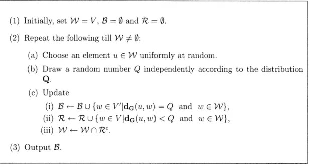
This section presents (e, A) decomposition algorithm for polynomially growing graphs for various choice of e and A. We will describe algorithm for node-based (e, A) decomposition. This will immediately imply algorithm for edge-based decomposition for the following reason: given G = (V, E) with growth rate p(G), consider a graph

of its edges

g

g

The node-based decomposition algorithm for G will be described for the metric space on V with respect to the shortest path metric dG introduced earlier. Clearly, it is not possible to have (e, A) decomposition for any e and A values. As will become clear later, it is important to have such decomposition for e and A being not too large. Therefore, we describe algorithm for any e > 0 and an operational parameter

K, which will depend on e and the growth rate p and the corresponding constant C of the graph. We will show that our algorithm will output (e, A)-decomposition

where A will depend on e and K.

Given e and K, define a random variable Q over {1,..., K} as

[ (l-s)-iE iflli<K

P[Q = i] = 1

(1 -) K- 1 ifi=K

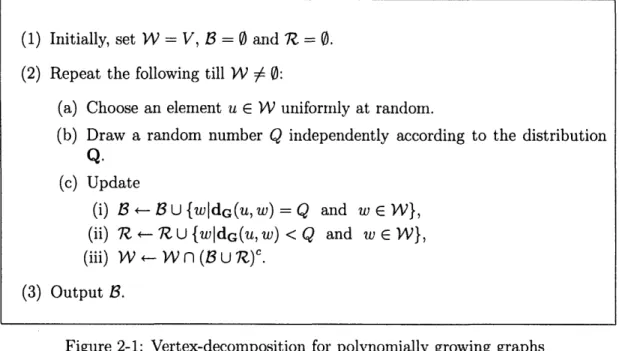
The graph decomposition algorithm POLY-V (e, K) described next essentially does the following. The algorithm performs iteratively. Initially, all vertices are colored white. If there is any white vertex, choose any of them arbitrarily. Let u be the chosen vertex. Draw an independent random number Q as per distribution Q. Select all white vertices that are at distance Q from u in B and color them blue; color all white vertices at distance < Q from u (including u itself) as red. Repeat this process until no more white vertices are left. Output B (i.e. blue nodes).

POLY-V (e, K)

(1) Initially, set

W =

V, B

=

0 and R = 0.

(2) Repeat the following till W

$

(a) Choose an element u E W uniformly at random.

(b) Draw a random number Q independently according to the distribution

Q.

(c) Update

(i) B+-BU {wldG(u,w) =Q and wE W}, (ii) 7I R U {wldG(u, w) < Q and

w

(3) Output B.

Figure 2-1: Vertex-decomposition for polynomially growing graphs

Precise description of the algorithm is in Figure 2-1. We will set

K = K(e, p, C) = 8Plog + - logC + log +2.

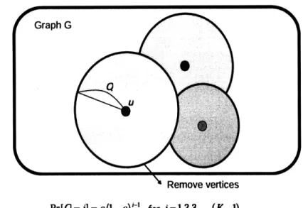
This definition is exploited in the proof of Lemma 4. Figure 2-2 explains the algorithm POLY-V up to three choices of u.

Lemma 4 Given graph G with growth rate p = p(G) and the corresponding constant C, and E E (0,1), the output of the POLY-V(e, K) becomes a (2e, CKP)

vertez-decomposition of G.

Proof. To prove that the random output set B C V of the algorithm with parameters (E, K(e, p)) we need to establish properties (a) and (b) of Definition 5.

Proof of (a). To prove (a), we state and prove the following Claim.

Claim 1 Consider metric space

g

Q.

Remove vertices

Pr[Q=i]=(1-) - for i=1,2,3...,(K-1)

Figure 2-2: The first three iterations in the execution of POLY-V.

any v E V,

P[v

e

B]

5

e + PKIBG(v, K)I,

where BG(v, K) is the ball of radius K in

g

with respect to the dG, and PK

(1

e)K

Proof. The proof is by induction on the number of points n over which the metric

space is defined. When n

=

1, the algorithm chooses only point as uo in the initial

iteration and hence it can not be part of the output set B. That is, for this only

point, say v,

P[v

e

B]

=

0 < E + PKIB(v, K)I.

Thus, we have verified the base case for induction (n =

1).

As induction hypothesis, suppose that the Claim 1 is true for any metric space

on n points with n < N for some N > 2. As the induction step, we wish to establish

that for a metric space

= (V,

with IVI

=

N, the Claim 1 is true. For this,

consider any point v E V. Now consider the first iteration of the POLY-V applied

to g. The algorithm picks u

E V uniformly at random in the first iteration. Given

v, depending on the choice of uo we consider four different cases (or events). We will

show that in these four cases,

P[v 1B] E + PK IBG(v, K)

holds.

Case 1. This case corresponds to event El where the chosen random uo is equal to

point v of our interest. By definition of the algorithm, under the event El, v will never be part of output set B. That is,

P[v BE11] = 0 < E + PIB(v, K)j.

Case 2. Now, suppose uo is such that v u uo and dG(uo, v) < K. Call this event

E2-Further, depending on choice of random number Qo, define the following events

E21 = {dG(UO, v) < Qo}, E22 = {dG(uLO, v) = Q0}, and E23 = {dG ('o, v) > Qo}

-By definition of the algorithm, when E21 happens, v is selected as part of R1 and

hence v can never be a part of output B. When E22 happens, v is selected as part of

B1 and hence it is definitely a part of output set B. When E23 happens, v is neither

selected in set R1 nor selected in set B1. It is left as an element of the set W1. This

new set W1 has points less than N. The original metric dG is still the metric on the points3 of W1. By definition, the algorithm only cares about (W1, dG) in the future and it is not affected by its decisions in past. Therefore, we can invoke induction hypothesis which implies that if event E23 happens then the probability of v E B is bounded above by e+PK IB(v, K) . Finally, let us relate the P[E21 E2] with P[E22 E2].

Suppose dG(uo, v) = e < K. By definition of probability distribution of Q, we have

P[E22 E2 = E( -)1 , (2.5)

3

Note the following subtle but crucial point. We are not changing the metric de after we remove points from original set of points as part of the POLY-V.

P[E21

1E

]

IE

Let q - IP[E2 1

!E

[v E

BIE

]

=

P[v

e

BIE

n

E

]P[E

IE

] +

P[v

e

BlE

n

E

]P[E

1E

]

+

P[v E

B

lE

n E2]P[E

IE2]

0 x q+1 x + ( + PKIB(v, K)) 1

-=

e

+ PKIB(v, K)I + 1

(e

-

e

- PK B(v, K)I)

qPKB(v,K)

1-6

<

E + PKIB(v, K)I.

Case 3. Now, suppose uo 3 v is such that dc(uo, v) = K. We will call this event E3.

Further, define the event E3 1 = {Qo = K}. Due to the independence of selection of Qo, P[E3 1

IE

P[v

E

BI]E

]

=

P[v

e BIE

n E

]P[EaiIE] +

P[v

BIE

n

E

]P[E.

IE

]

= 1 x PK + P[v E BIEI n E3](1 - PK).

Under the event E3, nE 3, we have v E W1, and the remaining metric space (W1, dG).

This metric space has < N points. Further, the ball of radius K around v with respect to this new metric space has at most IB(v, K)I - 1 points (this ball is with respect to the original metric space

g

P[v

BJEg n E~

] 5 e+PK(IB(v, K)I

1).

That is,

(2.6)

(2.7)

(2.8)