DeepStreaks: identifying fast-moving objects in the Zwicky
Transient Facility data with deep learning
Dmitry A. Duev,
1
?
Ashish Mahabal,
1
Quanzhi Ye,
1,2
Kushal Tirumala,
3
Justin Belicki,
4
Richard Dekany,
4
S. Frederick,
5
Matthew J. Graham,
1
George Helou,
2
Russ R. Laher,
2
Frank J. Masci,
2
Thomas A. Prince,
1
Reed Riddle,
4
Philippe Rosnet,
6
Maayane T. Soumagnac,
7
1Division of Physics, Mathematics, and Astronomy, California Institute of Technology, Pasadena, CA 91125, USA 2IPAC, California Institute of Technology, MS 100-22, Pasadena, CA 91125, USA
3Division of Engineering and Applied Science, California Institute of Technology, Pasadena, CA 91125, USA 4Caltech Optical Observatories, California Institute of Technology, Pasadena, CA 91125, USA
5Department of Astronomy, University of Maryland, College Park, MD 20742, USA 6Universit´e Clermont Auvergne, CNRS/IN2P3, LPC, Clermont-Ferrand, France 7Benoziyo Center for Astrophysics, Weizmann Institute of Science, Rehovot, Israel
Accepted 2019 April 13. Received 2019 April 11; in original form 2019 February 25
ABSTRACT
We present DeepStreaks, a convolutional-neural-network, deep-learning system designed to efficiently identify streaking fast-moving near-Earth objects that are de-tected in the data of the Zwicky Transient Facility (ZTF), a wide-field, time-domain
survey using a dedicated 47 deg2camera attached to the Samuel Oschin 48-inch
Tele-scope at the Palomar Observatory in California, United States. The system demon-strates a 96-98% true positive rate, depending on the night, while keeping the false positive rate below 1%. The sensitivity of DeepStreaks is quantified by the perfor-mance on the test data sets as well as using known near-Earth objects observed by ZTF. The system is deployed and adapted for usage within the ZTF Solar-System framework and has significantly reduced human involvement in the streak identifica-tion process, from several hours to typically under 10 minutes per day.
Key words: methods: data analysis – asteroids: general – surveys
1 INTRODUCTION AND CONTEXT
Solar System small bodies (SBs) in the context of orbiting asteroids and comets are believed to be remnants of our So-lar System’s early days, holding clues about its formation and evolution. A subclass of SBs known as the near-Earth objects (NEOs) is of particular interest especially since some of them pose a hazard due to a non-negligible probability of collision with the Earth (Desmars et al. 2013).1 Luckily, collisions with kilometer-sized objects that would have dev-astating effects are rare. However, the impact frequencies for smaller objects that could still cause significant damage are much higher.
Our knowledge of the kilometer-sized NEO population
? E-mail: [email protected] (DAD)
1 Of about 19,600 NEOs known as of January 2019, roughly 1,900 are classified as potentially hazardous asteroids (PHAs).
is fairly complete. However, the current NEO completeness for 140 m objects is only about 30% and drops rapidly with decreasing object size (Vereˇs & Chesley 2017).2To date, only a relatively small number of NEOs with sizes of 50 m have been discovered, but the vast majority, as many as 98%, of the estimated quarter million 50 m class NEOs, have not been found yet.
Detection of small NEOs poses a significant challenge as they are either very faint while far away from the Earth, or they have high apparent motion when close and bright enough to be detected. Objects that approach the Earth within 15 lunar distances typically move at a rate of > 10◦ per day (Vereˇs et al. 2012). These “Fast-Moving Objects” (FMOs) would trail on typical survey exposures (usually
2 In 2005, the United States Congress directed NASA to find at least 90 percent of potentially hazardous NEOs sized 140 meters or larger by the end of 2020.
domain sky survey that visits the entire visible sky north of −30◦declination every three nights in the g and r bands, and at higher cadences in selected sky regions including observa-tions with the i-band filter (Bellm et al. 2019;Graham et al. 2019). The new 576 megapixel camera with a 47 deg2 field of view (Dekany & Smith 2019), installed on the Samuel Oschin 48-inch (1.2-m) Schmidt Telescope, can scan more than 3750 deg2 per hour, to a 5σ detection limit of 20.7 mag in the r band with a 30-second exposure during new moon.
The raw data are transferred to the Infrared Processing and Analysis Center (IPAC) at the California Institute of Technology (Caltech) and processed in real time. The ZTF Science Data System (ZSDS) housed at IPAC consists of the data processing pipelines, data archives, infrastructure for long-term curation, and the services for data retrieval and visualization (Masci et al. 2019).
A part of the ZSDS, the ZTF Streak pipeline (ZStreak) focuses on the detection of streaked objects. A detailed de-scription of ZStreak is given inYe et al.(2019), and is based, in part, on earlier prototype work byWaszczak et al.(2017). In essence, the pipeline first detects plausible streak can-didates in difference images3 by searching for contiguous bright pixels that exceed a signal-to-noise threshold of 1.5 sigma and whose spatial distribution is approximately linear according to an estimate of the Pearson correlation coeffi-cient4. It then tries to fit a streaked point-spread function (PSF). If successful, a manually selected set of features per streak is passed through a Random-Forest (RF) machine-learning (ML) classifier that assigns a score from zero to one representing the likelihood of the streak being real (which corresponds to a score of one). A threshold of 0.05 is adopted, which is about 96 − 98% complete at this score in terms of detecting real FMOs present in the raw-streak sample. The candidates passing this threshold are vetted for real detec-tions by human scanners on a daily basis. The detected real streaks are linked and if plausible linkages are found, an or-bit fit is attempted. Finally, if the oror-bital solution converges and the corresponding “track” is not associated with human-made objects, the observations (of both known and newly discovered objects) are submitted to the International
As-3 Constructed by “properly” subtracting a reference (template) image from a science exposure image according toZackay et al. (2016).
4 Currently, alternative streak detection approaches are being in-vestigated, including those described inNir et al.(2018)
significantly reduces the number of false positives.
2 DEEPSTREAKS: A DEEP LEARNING FRAMEWORK FOR STREAK
IDENTIFICATION
The term “artificial intelligence” (AI) usually refers to sit-uations where machines solve problems commonly associ-ated with human intelligence, such as image recognition and classification. Machine learning, often recognized as a sub-set of AI, refers to the cases where machines learn from the data rather than being explicitly programmed. Finally, Deep Learning (DL) is a subset of ML that employs many-layer artificial neural networks.
DL has gained popularity in recent years thanks to the advances in both related hardware (graphical and tensor processing units – GPUs and TPUs) and software (program-ming frameworks such as TensorFlow, PyTorch and others) coupled with the advent of Big Data. As a result, DL-based systems are starting to outperform humans in a number of areas. In particular, a subclass of DL systems, the convo-lutional neural networks (CNNs), have been demonstrated to yield outstanding performance in image recognition and classification tasks. For a thorough introduction of CNNs re-fer to, for example,Lieu et al.(2018) and references therein. In this paper, we present DeepStreaks, a CNN-based deep learning framework developed to efficiently identify streaking FMOs in the ZTF data.
2.1 Architecture
Given the very practical goal of this work, we have chosen to explore two possible DL-system architectures. In the first approach, the problem of identifying a plausible streak is divided into three simpler sub-problems that are each solved by a dedicated group of classifiers:
(i) “rb”: identify all streak-like objects, including the ac-tual streaks from fast-moving objects, long(er) streaks from satellites, and cosmic rays. Assign a real(r b= 1)/bogus(rb = 0) score.
(ii) “sl”: identify short streak-like objects, including the actual streaks from fast moving objects and artifacts such as cosmic rays. Assign a short(sl= 1)/long(sl = 0) score.
Figure 1. Architecture of the simple custom VGG6 model. ReLU activation functions are used for all five hidden trainable layers; a sigmoid activation function is used for the output layer. Dropout is used for regularization.
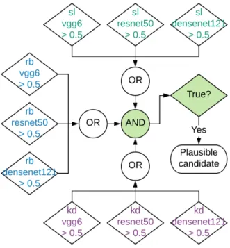
Figure 2. Decision logic used by DeepStreaks to identify plausi-ble streaks. The proplausi-blem is split into three simpler sub-proplausi-blems, each solved by a dedicated group of classifiers assigning real vs. bogus (“rb”), short vs. long (“sl”), and keep vs. ditch (“kd”) scores. At least one member of each group must output a score that passes a pre-defined threshold. See Section2.1for details.
(iii) “kd”: identify real streaks produced by FMOs. As-sign a keep(k d= 1)/ditch(kd = 0) score.
We note that the overwhelming majority of “long” streaks are produced by human-made objects. A streak is considered long if it extends outside of the cutout image6. This comprises objects that move faster than 125-175 de-grees per day, depending on the streak positional angle.
The classifiers used in the second, one-shot (“os”)
ap-6 By design, at least some part of the streak is near the center of the cutout image.
Figure 3. Decision logic to identify plausible streaks used in the one-shot (“os”) classification approach. See Section2.1for details.
proach that we explored, solve the classification problem di-rectly.
Within each group of classifiers we have chosen to use three different CNN models:
(i) A simple custom VGG7-like sequential model (“VGG6”) (Simonyan & Zisserman 2014) (see Fig.1for de-tails). The model has six layers with trainable parameters: four convolutional and two fully-connected. The first two convolutional layers use 16 filters each while in the second pair, 32 filters are used. To prevent over-fitting, a dropout rate of 0.25 is applied after each max-pooling layer and a dropout rate of 0.5 is applied after the second fully con-nected layer. ReLU activation functions8 are used for all five hidden trainable layers; a sigmoid activation function is used for the output layer.
(ii) A custom 50-layer deep model based on residual con-nections (“ResNet50”), which are concon-nections that add mod-ifications with each layer, rather than completely changing the signal. The implementation details are given inHe et al.
7 This architecture was first proposed by the Visual Geometry Group of the Department of Engineering Science, University of Oxford, UK
8 Rectified Linear Unit – a function defined as the positive part of its argument
Architectures that are more complex than ResNet50 and DenseNet121 have been demonstrated to yield better performance on large public image data sets such as Im-ageNet (Deng et al. 2009), however, these models are not necessarily better at generalizing to other data sets ( Korn-blith et al. 2018).
The differenced cutout images with raw streaks pro-duced by the ZStreak pipeline are gray-scale and of size 157 by 157 pixels (or smaller if a raw streak is detected close to the field edge) at a plate scale of 100 per pixel. The in-put image size of all our CNN models is 144x144x1, so the cutouts are down-sampled accordingly. All individual mod-els are evaluated on all raw streaks. In the first approach (“rb”+“sl”+“kd”), for a streak to be marked as a plausible real candidate, for each classifier group, at least one group member must output a score greater than a pre-set thresh-old (see Figure2and Section2.2). Similarly, in the “os” ap-proach, at least one classifier must report a score that passes a threshold (see Figure3and Section2.2).
2.2 Data sets, training, and performance
To accelerate data labelling, we developed a simple web-based tool we called Zwickyverse9 that provides both effi-cient API and GUI. The tool is easy to deploy thanks to containerization using Docker software10and it allows quick integration of newly-labelled data sets into the model train-ing workflow. All data labelltrain-ing for this work was done ustrain-ing Zwickyverse.
We started with a training set that consisted of 1,000 differenced images with streaks that span a period of time from the start of the survey in March 2018 until the end of 2018, identified as real by human scanners; 8,270 synthetic streak images generated by implanting a streaked PSF into a bogus image following Ye et al. (2019); and 6,000 “bo-gus” images of different kinds: streaks from satellites and airplanes (which are typically long and, frequently, of vary-ing brightness) and false streak detections caused by, for ex-ample, masked bright stars, bad subtractions, cosmic rays, “dementors”, and “ghosts” (see Figure4). This data set was used to train an initial set of “rb” classifiers that separate all sorts of streak-like objects from false detections. Next, we evaluated the resulting classifiers on a month of ZTF data, sampled images that received low, intermediate, and
9 https://github.com/dmitryduev/zwickyverse 10 https://www.docker.com/
richment” and classifier retraining campaigns aimed at cov-ering a wider range of weather conditions and tuning the classifier performance. We plan to continue conducting such campaigns in the future.
Separately, the training data set for the “os” (one-shot) classifiers contains all true short streaks detected by ZTF from the start of the survey until the end of 2018, the syn-thetic streaks from the initial data set, and a set of images covering the whole range of possible false streak and bogus images.
As of February 2019, the training set for the “rb” classi-fiers contains 11,857 images of streak-like objects (including the actual streaks from FMOs, long(er) streaks from satel-lites, and cosmic rays) and 13,449 non-streak images; for the “sl” classifiers – 5,168 long and 11,246 short streak images; for the “kd” classifiers – 14,154 “false” and 10,621 “true” im-ages; and finally for the “os” classifiers – 16,808 “false” and 10,621 “true” images.
DeepStreaks is implemented using TensorFlow software and its high-level Keras API (Abadi et al. 2015;Chollet et al. 2015). For all models that we trained, we used the binary cross-entropy loss function, the Adam optimizer (Kingma & Ba 2014), a batch size of 32, and a 81%/9%/10% train-ing/validation/test data split. The training image data were weighted per class to mitigate the imbalances in the data sets. The images may be flipped horizontally and/or verti-cally at random. No random rotations and translations were added since those may change the class of the streak for the “sl” and “kd” classifiers. As it is, the position angles of the streaks adequately sample the range from 0 to 360 degrees. We used the early stopping technique to finish train-ing if no improvement in validation accuracy was observed over many epochs. As a result, the models were trained for 150-300 epochs. For training, we used an on-premise Nvidia Tesla P100 12G GPU. Training a single neural network for 300 epochs on ∼ 25k images takes about 1.5 hours for the VGG6 architecture, 8 hours for ResNet50, and 10 hours for DenseNet121.
Figure5shows training (left panel) and validation (right panel) accuracy for all the models that are deployed in pro-duction as of January 2019. While the training accuracy for most classifiers reaches over 99% level after several dozen epochs, the validation accuracy generally stays in the 96-98% range for the “rb” and “sl” classifiers, while the “kd” classifiers reach 94-97% validation accuracy. We believe the latter is due to the intrinsic difficulty of the problem to dis-tinguish real short streaks from FMOs observed in excellent
(a) Bad subtraction (b) Cosmic ray (c) “Dementor” (d) “Ghost” (e) Masked star (f) Satellite trail Figure 4. Examples of different classes of bogus streak detections.
Figure 5. Training (left panel) and validation (right panel) accuracy for all the models that are deployed in production as of January 2019.
Figure 6. ROC curves for all the models that are deployed in production as of January 2019. The right panel displays a zoomed-in view of the top left corner of the full plot shown on the left panel.
(sub-arcsecond) seeing from certain cosmic rays. In our ex-perience, this task is similarly arduous for human scanners. The test performance of the resulting classifiers as a function of the score threshold is shown on the receiver op-erating characteristic (ROC) curve, see Fig.6. Evidently, a score threshold of 0.5 that is adopted for all classifiers in DeepStreaks yields 96-98% true positive rate (TPR) on the test sets while keeping the false positive rate (FPR) low.
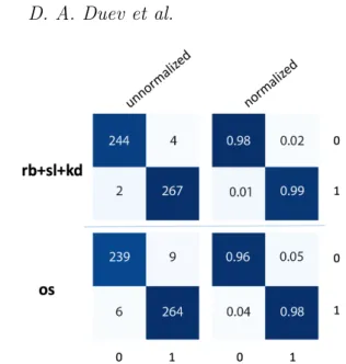
To assess the performance of the ensemble versus the one-shot classification approach, we constructed a separate test set consisting of 248 bogus and 270 real streak images and evaluated the decision logic depicted in Figures2 and
3. As can be seen from the resulting confusion matrices (see
Fig.7), the approaches show similar performance in terms of precision versus recall on this test set. However, the en-semble (“rb”+“sl”+“kd”) system demonstrated a much better performance when evaluated on all the raw streak cutouts produced by ZTF from December 15, 2018 – January 15, 2019, which covered a wide range of weather/seeing condi-tions. Concretely, out of the total of 7 million raw streaks, about 33 thousand (0.5% of the total) were declared plausi-ble candidates by the ensemplausi-ble system, whereas the one-shot system output about 8 times more (250 thousand or 3.5% of the total). Additionally, we ran a sanity check by evaluating the classifiers on a random sample of eight thousand images from the public ImageNet data set. The resulting false
pos-Figure 7. Un-normalized (left column) and normalized (right column) confusion matrices for the ensemble (top row) versus the one-shot (bottom row) classification approach evaluated of a test set of 248 bogus and 270 real streak images from both natural and human-made FMOs. The top-left corner of the matrices shows the number/rate of true negatives, the top-right – the number/rate of false positives, the bottom-left – the number/rate of false neg-atives, and the bottom-right – the number/rate of true positives.
itive rate for the ensemble system turned out to be exactly zero, however for the one-shot system, the FPR was around 1%. For these reasons, DeepStreaks employs the ensemble approach in production.
We chose not to use transfer learning to initialize or freeze layer weights for the deep models and trained all our models from scratch. The reason is that the available pre-trained networks are pre-trained on drastically different image data sets and thus do not necessarily capture the features relevant to this work.
Figure 8 shows the Venn diagram of the number of streaks that pass different DeepStreaks’ sub-thresholds and the final number of plausible candidates (see Fig.2) in ZTF data from December 15, 2018 - January 15, 2019. We note that ZTF did not observe for 11 nights during that period due to bad weather. Human scanners marked 270 out of 33 thousand plausible candidates as real FMO streaks.
While providing a similar sensitivity, DeepStreaks demonstrates a 50× better performance than the original random forest-based classifier used in the ZStreak pipeline in terms of the false negative rate: 1.7 million raw streaks (25% of the total) were designated plausible candidates by the RF classifier in the same time period. This reduces dras-tically the time humans have to spend scanning for streaks – from hours to typically under 10 minutes per day.
3 DISCUSSION
The real-time production service that runs DeepStreaks in inference mode is containerized using Docker software. The classifiers are evaluated on batches of raw streak images to utilize vectorization. All individual scores together with the meta-data associated with each streak are saved to a
Mon-Figure 8. Venn diagram showing the number of streaks that pass DeepStreaks’ sub-thresholds and the final number of plausible candidates. ZTF data from December 15, 2018 – January 15, 2019. ZTF did not observe for 11 nights during that period due to bad weather. The final number of “good” candidates output by DeepStreaks (33 thousand) amounts to 0.5% of the total number of streaks produced by ZTF (compare to 1.7 million, or 25% of the total output by the RF classifier). 270 streaks out of the 33 thousand plausible candidates were marked as real FMO streaks by human scanners.
goDB NoSQL database11. We also built a simple flask12 -based web GUI that provides easy access to the database.
The ZTF FMO Marshal (the web interface of ZStreak) queries the DeepStreaks database every minute and posts DeepStreaks-identified objects in real-time. One or more hu-man scanners then review the stamps on the Marshal and save objects that are potentially interesting for further ex-amination. Compared to the procedure described inYe et al.
(2019), the introduction of DeepStreaks has reduced the number of stamps posted on the Marshal by 50 − 100×. This vastly reduces the burden on human scanners, and facili-tates near-real-time identification of potentially interesting objects.
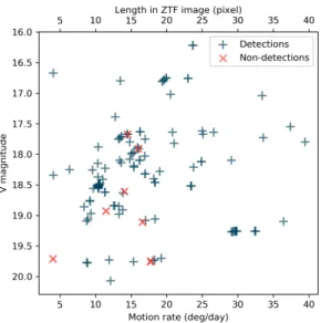
To quantify the completeness of DeepStreaks identi-fications, we evaluated it on streak images of known real NEOs detected by the ZTF Streak pipeline from October 2018 – January 2019 (see Fig.9). Out of 210 such streaks, 202 (96%) were correctly classified. We note that the RF classifier initially used in ZStreak with a threshold of 0.05 demonstrates similar TPR on this data set.
We observe a 10-20% reduction in the number of false positives after each “dataset enrichment” campaign that we carried out (see Section2.2). We will continue conducting such campaigns in the future to further reduce the FPR. The nightly variation in the TPR (96-98%) appears to be random, however such factors as airmass, seeing or Moon phase etc. may play a role here. It is hard to quantify the effect of these factors at this point due to small number
11 https://www.mongodb.com/
Figure 9. Completeness of DeepStreaks identifications using known NEOs observed by ZTF in October 2018 – January 2019. Out of 210 streaks from real NEOs detected by the ZTF Streak pipeline at IPAC, 202 (96%) are correctly classified. ZTF plate scale is 100per pixel.
statistics, but we plan to perform a detailed investigation in the future.
As of February 1, 2019, 15 NEOs have been discovered with DeepStreaks, including 2019 BE5, the fastest-spinning asteroid discovered to date that has a rotational period of 12 seconds (W. Ryan, private comm.), and 2019 BF5, a
PHA. Table1 summarizes the confirmed NEO discoveries. Listed are asteroid designation assigned by the Minor Planet Center, discovery date, V -magnitude, apparent motion rate, flyby distance, orbital type and absolute magnitude. Figure
10shows examples of streaks from real fast-moving objects, both natural and human-made, identified by DeepStreaks. The data were taken under a wide range of seeing conditions (FWHM from 1.5” to 4”) and spanned across December 2018 – January 2019.
We have demonstrated that by putting together a few simulations, large amounts of data from ZTF, fast comput-ing, and a few deep learning models we can improve the efficiency of detecting streaking asteroids by a couple or-ders of magnitude, saving tens of human-hours per week at the same time. Our method can be equally easily applied to other data sets, many of which are publicly available. We will continue striving to find fainter objects in ZTF data trying to push for completeness. The additional epochs we gather for known objects will also help build better orbits and hopefully provide early warning should any err in the direction of Earth.
DeepStreaks code and pre-trained models are available athttps://github.com/dmitryduev/DeepStreaks
ACKNOWLEDGEMENTS
D.A. Duev acknowledges support from the Heising-Simons Foundation under Grant No. 12540303. Q.-Z. Ye is sup-ported by the GROWTH project funded by the National
Sci-ence Foundation under Grant No. 1545949. Based on obser-vations obtained with the Samuel Oschin Telescope 48-inch Telescope at the Palomar Observatory as part of the Zwicky Transient Facility project. Major funding has been pro-vided by the U.S. National Science Foundation under Grant No. AST-1440341 and by the ZTF partner institutions: the California Institute of Technology, the Oskar Klein Centre, the Weizmann Institute of Science, the University of Mary-land, the University of Washington, Deutsches Elektronen-Synchrotron, the University of Wisconsin-Milwaukee, and the TANGO Program of the University System of Taiwan. AM acknowledges support from NSF (1640818 and AST-1815034).
The authors are grateful to Eran Ofek for useful discus-sions.
REFERENCES
Abadi M., et al., 2015, TensorFlow: Large-Scale Machine Learning on Heterogeneous Systems,https://www.tensorflow.org/ Bellm E. C., et al., 2019,Publications of the Astronomical Society
of the Pacific,131, 018002
Chollet F., et al., 2015, Keras,https://keras.io
Dekany R., Smith R., 2019, The Zwicky Transient Facility: Ob-serving System, In prep.
Deng J., Dong W., Socher R., Li L.-J., Li K., Fei-Fei L., 2009, in CVPR09.
Desmars J., Bancelin D., Hestroffer D., Thuillot W., 2013, As-tronomy and Astrophysics,554, A32
Graham M. J., et al., 2019, arXiv e-prints,p. arXiv:1902.01945 He K., Zhang X., Ren S., Sun J., 2015, arXiv e-prints, p.
arXiv:1512.03385
Huang G., Liu Z., van der Maaten L., Weinberger K. Q., 2016, arXiv e-prints,p. arXiv:1608.06993
Jedicke R., Schunova E., Vereˇs P., Denneau L., 2013, Prepared for NASA HEOMD and the Jet Propulsion Laboratory, 24 Kingma D. P., Ba J., 2014, arXiv e-prints,p. arXiv:1412.6980 Kornblith S., Shlens J., Le Q. V., 2018, arXiv e-prints, p.
arXiv:1805.08974
Lieu M., Conversi L., Altieri B., Carry B., 2018, preprint, p. arXiv:1807.10912(arXiv:1807.10912)
Masci F. J., et al., 2019,Publications of the Astronomical Society of the Pacific,131, 018003
Nir G., Zackay B., Ofek E. O., 2018,AJ,156, 229
Simonyan K., Zisserman A., 2014, arXiv e-prints, p. arXiv:1409.1556
Vereˇs P., Jedicke R., Denneau L., Wainscoat R., Holman M. J., Lin H.-W., 2012,PASP, 124, 1197
Vereˇs P., Chesley S. R., 2017,AJ,154, 12 Waszczak A., et al., 2017,PASP, 129, 034402
Ye Q.-Z., Masci F. J., Lin H. W., et al., 2019, Towards Efficient Detection of Small Near-Earth Asteroids Using the Zwicky Transient Facility (ZTF), Submitted to PASP.
Zackay B., Ofek E. O., Gal-Yam A., 2016,ApJ,830, 27 This paper has been typeset from a TEX/LATEX file prepared by the author.
2019 BK2 2019 Jan. 26 18.4 30 2.8 Apollo 26.8 2019 BY3 2019 Jan. 28 18.9 15 3.2 Apollo 27.4 2019 BL4 2019 Jan. 28 19.7 10 2.6 Apollo 27.7 2019 BC5 2019 Jan. 31 19.0 15 7.0 Apollo 25.4 2019 BD5 2019 Jan. 31 17.7 25 2.8 Apollo 26.7 2019 BE5 2019 Jan. 31 15.1 50 3.0 Aten 25.0 2019 BF5 2019 Jan. 28 18.0 20 9.5 Apollo 21.5
Figure 10. Examples of streaks from real objects, both natural and human-made, identified by DeepStreaks in December 2018 - January 2019. The data were taken under a wide range of weather/seeing conditions (FWHM from 1.5” to 4”).