HAL Id: halshs-00825303
https://halshs.archives-ouvertes.fr/halshs-00825303
Preprint submitted on 23 May 2013
HAL is a multi-disciplinary open access
archive for the deposit and dissemination of sci-entific research documents, whether they are pub-lished or not. The documents may come from teaching and research institutions in France or abroad, or from public or private research centers.
L’archive ouverte pluridisciplinaire HAL, est destinée au dépôt et à la diffusion de documents scientifiques de niveau recherche, publiés ou non, émanant des établissements d’enseignement et de recherche français ou étrangers, des laboratoires publics ou privés.
An Economic Evaluation of Model Risk in Long-term
Asset Allocations
Christophe Boucher, Gregory Jannin, Bertrand Maillet, Patrick Kouontchou
To cite this version:
Christophe Boucher, Gregory Jannin, Bertrand Maillet, Patrick Kouontchou. An Economic Evaluation of Model Risk in Long-term Asset Allocations. 2013. �halshs-00825303�
Laboratoire d'Economie d'Orléans – UMR CNRS 7322 Faculté de Droit, d'Economie et de Gestion, Rue de Blois, B.P. 26739 – 45067 Orléans Cedex 2 - France
Document de Recherche
n° 2013-03
« An Economic Evaluation of Model Risk
in Long-term Asset Allocations »
Christophe BOUCHER
Grégory JANNIN
Bertrand MAILLET
Patrick KOUONTCHOU
An Economic Evaluation of Model Risk
in Long-term Asset Allocations
Christophe Boucherh Gregory Jannini Patrick Kouontchouj Bertrand Mailletk
Abstract
Following the recent crisis and the revealed weakness of risk management practices, regulators of developed markets have recommended that financial institutions assess model risk. Standard risk measures, such as the Value-at-Risk (VaR), emerged over recent decades as the industry standard for risk management and have today become a key tool for asset allocation. We illustrate and estimate model risk, and focus on the evaluation of its impact on optimal portfolios at various time horizons. Based on a long sample of U.S. data, we find a non-linear relation between VaR model errors and the horizon that impacts optimal asset allocations.
Keywords: Model Risk, VaR, Long-term Asset Allocation, Safety First Criterion. JEL Classification: C14, C52, G11, G32.
Résumé
Suite aux récents épisodes de crise et les faiblesses constatées des pratiques de gestion des risques, les régulateurs des marchés financiers développés recommandent désormais que les établissements financiers évaluent le risque de modèle. Certaines mesures standard de risque extrême, telle que la Value-at-Risk (VaR), sont en effet considérées comme le standard de l'industrie pour la gestion des risques et elles sont devenues aujourd'hui un outil essentiel pour l'allocation d'actifs. Nous illustrons dans cet article l’impact du risque de modèle sur les portefeuilles optimaux à différents horizons temporels. A partir d’un long échantillon de données américaines, nous montrons qu’il existe en effet une relation non linéaire entre les erreurs de modèle lié aux calculs des VaR et l'horizon de placement, qui se traduit lui-même par un impact sur les allocations d'actifs optimales.
Mots-clefs : risque de modèle, VaR, allocation d’actifs de long-terme, critère de prudence. Classification JEL : C14, C52, G11, G32.
h A.A.Advisors-QCG (ABN AMRO), Variances et Université de Lorraine (CEREFIGE), Faculté de Droit Économie Administration, Ile du Saulcy, 57045 METZ cedex 01. E-mail: christophe.boucher@univ-lorraine.fr. i Variances et Université de Paris-1 (PRISM). PRISM Sorbonne, 17 rue de la Sorbonne 75005 Paris. E-mail:
gregory.jannin@univ-paris1.fr.
jVariances et Université de Lorraine (CEREFIGE), Faculté de Droit Économie Administration, Ile du Saulcy, 57045 METZ cedex 01. E-mail: patrick.kouontchou@univ-lorraine.fr.
k
A.A.Advisors-QCG (ABN AMRO), Variances et Université d’Orléans (LEO/CNRS et IEF). Correspondance à : Bertrand Maillet, Université d’Orléans, Rue de Blois – BP 26739 – 45067 ORLEANS Cedex 2, France. Email: bertrand.maillet@univ-orleans.fr.
An Economic Evaluation of Model Risk
in Long-term Asset Allocations
Abstract
Following the recent crisis and the revealed weakness of risk management practices, regulators of developed markets have recommended that financial institutions assess model risk. Standard risk measures, such as the Value-at-Risk (VaR), emerged over recent decades as the industry standard for risk management and have today become a key tool for asset allocation. We illustrate and estimate model risk, and focus on the evaluation of its impact on optimal portfolios at various time horizons. Based on a long sample of U.S. data, we find a non-linear relation between VaR model errors and the horizon that impacts optimal asset allocations.
1. Introduction
The recent global financial crisis has focused a great deal of attention on the risk management practices of financial institutions around the world1. Suddenly, too prudent risk models (during calm periods) have become too aggressive (in turbulent periods). A large variety of risk measures have been proposed in academic and practitioner literatures in order to avoid such a situation. Risk Measures such as Value-at-Risk (VaR) are currently used in various fields, namely, not only in the management policies and international regulations for the financial (Basel II) and insurance (Solvency II) sectors2, but also for asset allocation, especially for long-term investors (e.g. Monfort, 2008; Levy and Levy, 2009). The quality of risk measure estimates may considerably influence long-term asset allocation decisions, since assets are ranked and mixed on the basis of their risk-return at specific horizons.
This paper proposes an economical valuation of the consequences of model uncertainty on VaR estimates, based on a backtesting framework, and then examines the effects of the uncertainty of risk models on optimal portfolios at various time horizons. We propose a correction method that is not directly dependent on an assumed data generating
process, but rather on past failures of the model used. Our focus is essentially realized on VaR, but the analysis can also applied to other risk measures such as the Expected Shortfall. From a long sample of U.S. data, we find an inverse non-linear relation between VaR model errors and the horizon that impacts the optimal asset allocations.
While some papers have also considered the portfolio effects of parameter and model uncertainty (e.g. Barberis, 2000; Pástor and Stambaugh, 2012)3, risk estimate uncertainty has
received far less attention. Nevertheless, the Basel III committee has recently further recommended that most of the financial institutions evaluate model risk (BCBS, 2009). Indeed, model risk is commonly disregarded in the development of risk models by the financial industry, although well-known for peculiar price processes (e.g. Cont, 2006)4.
The outline of the paper is as follows. Section 2 defines and illustrates the model risk in VaR estimates. Section 3 explains our practical approach for calibrating adjusted Empirical VaRs that deal with the model risk. Section 4 presents the term-structure of model risk on VaR estimates and its impact on optimal portfolios at various time horizons. Section 5 concludes.
2. The Model Risk of VaR
The implications of over - or under - risk exposure estimation of risks are diametrically different for regulators and risk takers. However, prudential regulation leads to reconcile these conflicting interests so that both under and over-exposures to risk lead to inefficiency.
The amendment to the initial Basel Accord (BCBS, 1996) was designed to encourage and reward institutions for superior risk management systems. A backtesting procedure, that compares actual returns with the corresponding VaR forecasts, was introduced to assess the quality of internal models. The objective was to monitor the frequency of the so-called
“exceptions” when realized losses exceed the estimated VaR. Therefore, appropriately constructed accurate risk measures, particularly robust to model risks, are of paramount practical importance. Methods for the quantification of this type of risk are not nearly as well developed as methods for the quantification of market risk given a model, and the view is widely held that better methods to deal with model risk are essential to improve risk management and to reinforce the global international financial stability. Hence, the Basel III committee has proposed that financial institutions assess model risk, whether they come from some mis-specifications or estimation problems of risk models5. In the finance literature, the
term “model risk” frequently applies to uncertainty about the risk factor distribution (e.g. Boucher et al., 2012b). More precisely, in our context, model risk of risk models refers both to the range of plausible risk estimates, as well as the inability to properly forecast risk realizations.
The model risk of risk models mainly comes from parameter estimation errors and specification errors. The former are linked to the number of data points used to estimate an assumed model, while the latter refer to the model risk stemming from inappropriate assumptions about the form of the data generating process6.
We first present hereafter the “multiplication factor” mechanism (or the so-called “Traffic Light” approach) established by the Basel Committee (BCBS, 1996) to account for the model risk of VaR estimates and, secondly, illustrations of the model risk of VaR estimates based on three data generating processes.
Basel Accords and Model Risk
The Basel II Accord (BCBS, 1996) stipulates that the daily Capital Requirement, denoted CRqt, must be set at the higher of the previous day’s VaR or the average VaR over
60 1 1 1 max ; 60 t t t d d CRq VaR- k - VaR -= æ ö = ç ´ ÷ è
å
ø. (1)The multiplication factor, k, has to be set within a range of 3 to 4 depending on the supervisor’s assessment of financial institution’s risk management practices based on a simple backtest. The multiplication factor is determined by the number of times losses exceed the day’s VaR figure. The minimum multiplication factor of 3 can be interpreted as a compensation for both model risk and losses exceeding the VaR7. The increase in the
multiplication factor is then designed to scale up the confidence level implied by the observed number of exceptions to the 99% confidence level desired by the regulators.
In calculating the number of exceptions, financial institutions are required to compare the forecasted VaR numbers with realized profit and loss figures for the previous 250 trading days. For precision, the 1988 Basel Accord (BCBS, 1988) was also amended in 1996 to allow financial institutions to use internal models to determine their VaR, while these financial institutions must demonstrate that their internal models are sound (BCBS, 1996).
However, losses in most of the banks’ trading books during the last financial crisis have been significantly higher than the minimum capital requirements under the former Pillar I market risk rules, because VaR were underestimated. It led to the revision of the Basel II market risk framework (2009). A stressed VaR requirement was introduced, taking into account an observation period relating to significant losses.
Meanwhile, some recent empirical studies (see, for example, Berkowitz and O'Brien, 2002; Gizycki and Hereford, 1998; Pérignon et al., 2008; Pérignon and Smith, 2010) have indicated that some financial institutions (at the time) overestimated their market risks in disclosures to the appropriate regulatory authorities, which can imply a costly restriction to the banks trading activity. Financial institutions may prefer to report high VaR numbers to avoid the possibility of regulatory intrusions, while turbulent periods reveal that these prudent
VaR were ex post, in fact, too aggressive. This conservative risk reporting suggests that efficiency gains were feasible, at least before the last major market turmoil.
Model Risk of VaR Estimates
We briefly illustrate hereafter the model risk of VaR estimates, which is here defined in the following illustration as the consequences of two types of errors due to a model misspecification and a parameter estimation uncertainty. Various VaR computation methods exist in the literature, from non-parametric, semi-parametric and parametric approaches (e.g. Christoffersen, 2009). However, the Historical-simulated VaR computation is still one of the most used by practitioners (Christoffersen and Gonçalves, 2005; Sharma, 2012) and will serve as the main reference throughout this article.
Table 1 presents the Estimated VaR, as well as the mean, minimum and maximum errors on these Estimated VaR. Errors are defined by the differences between the “true” asymptotic VaR (based on simulated data generating processes) and the imperfect Historical-simulated estimated VaR (because the latter are approximately specified and estimated with a limited data sample). Three different rolling time-windows (250, 300 and 350 days in Panels A, B and C)8 and several levels of probability confidence thresholds (three columns for each
Panel) are considered. The results are presented for three data generating processes for the underlying stock price with various intensities of jumps (Brownian, Lévy and Hawkes9). Note that the auto-regressivity in jumps considered in the Hawkes’ process permits reproduction of the main documented characteristics of financial returns, such as sudden shocks, self-excitement, regimes, heteroskedasticity, the clustering of extremes, asymmetry and excess kurtosis.
Table 1
Estimated annualized VaR and Model-risk Errors (in %)
Panel A. 250 days Rolling
Window Calibration Panel B. 300 days Rolling Window Calibration Panel C. 350 days Rolling Window Calibration
Processes 95.00% 99.00% 99.90% 95.00% 99.00% 99.90% 95.00% 99.00% 99.90%
Mean Estimated VaR -24.79 -35.75 -43.96 -24.81 -35.88 -44.87 -24.8 -35.79 -45.65 Mean VaR Error .00 -.14 -5.30 .01 -.01 -4.39 .01 -.10 -3.60 Min VaR Error -8.01 -13.15 -22.67 -7.5 -11.77 -21.29 -6.43 -10.75 -21.72
1. Normal
Max VaR Error 9.19 25.94 37.89 8.81 16.67 31.72 7.89 16.87 37.62 Mean Estimated VaR -25.17 -39.16 -73.74 -25.17 -39.18 -78.39 -25.17 -38.44 -82.17 Mean VaR Error 2.57 5.08 -22.74 2.57 5.11 -18.09 2.58 4.36 -14.3 Min VaR Error -5.82 -10.51 -69.63 -4.83 -9.34 -68.03 -4.25 -8.95 -68.96
2. Normal with Jumps
Max VaR Error 12.67 92.67 103.49 11.72 91.24 107.98 10.84 82.48 119.98 Mean Estimated VaR -27.34 -44.79 -63.36 -27.17 -44.53 -65.28 -27.06 -43.99 -66.67 Mean VaR Error 3.62 7.30 -4.52 3.45 7.05 -2.61 3.34 6.50 -1.22 Min VaR Error -5.67 -12.71 -39.58 -4.53 -11.76 -37.58 -5.73 -12.25 -37.58
3. Normal with Auto-correlated Jumps
Max VaR Error 23.79 51.8 59.86 18.57 47.18 66.59 17.78 46.08 62.87 Source: Errors are defined as the difference between the “true” asymptotic simulated VaR and the Estimated VaR. These statistics were computed with a series of 250,000 simulated daily returns with a specific data generating process (1. Brownian, 2. Lévy and 3. Hawkes), averaging the parameters estimated in Aït-Sahalia et al. (2012, Table 5, i.e. β=41.66%, λ3=1.20% and γ=22.22%), and ex post recalibrated for
sharing the same first two moments (i.e. μ=.12% and σ=1.02%) and the same mean jump intensity (for the two last processes such as 2 3
t t J
J = - which leads after rescaling here, for instance, to an intensity of the Levy, such as: λ2=1.06%). Using several rolling windows (250 daily
returns for Panel A, 300 daily returns for Panel B and 350 daily returns for Panel C), annualized Estimated VaR at the 95.00%, 99.00% and 99.90% confidence levels are presented in this table. The first column in each block related to a process represents the Mean Estimated VaR with specification and estimation errors, whilst the following cells indicate the mean-minimum-maximum of the adjustment term corresponding to the observed differences between the Imperfect Historical-simulated Estimated VaR, empirically recovered in 250,000 draws of limited samples of 250, 300 or 350 daily returns (Panel A, B and C), and the asymptotic (true) VaR (computed with the 250,000 data points of the full original sample for each process). Per convention, a negative adjustment term in the table indicates that the Estimated VaR (negative return) should be more conservative (more negative); see Aït-Sahalia et al. (2012) and Boucher et al. (2012a) for more details. Simulations by the authors.
As expected, the estimated VaR is an increasing function of the confidence level and of the presence of jumps in the process (Lévy and Hawkes cases). For a large number of trials, the mean bias of the Historical-simulated method is quite small (inferior to 1% in relative terms) in the Normal case. By contrast, this mean bias is quite large when jumps are considered (with an amplitude from 10% to 30% in relative terms10). Moreover, the range of
model-risk errors is, as expected, more important when a small sample is considered. It appears that the difference between Max VaR Error and Min VaR Error (the range of error) decreases with the number of days considered in the rolling window calibration, whatever the data generating process and the confidence level.
The observed range of potential relative errors (the difference between the maximum and minimum estimated errors divided by the estimated VaR) is substantial in our
experiments, representing between around 50% of the VaR levels in the best case (for the simple Gaussian data generating process over the longer sample) to as high as 263% in the worst case scenario (for the simple jump process over the shorter sample). Furthermore, the potential relative under-estimation of the “true” VaR (an over-aggressive estimated VaR) is, in the main, large (ranging from 10% to 30%, depending on the sample length and the quantile considered). These results suggest that the Historical-simulated VaR should be corrected when safely taking into account the riskiness of risk models11.
3. A Simple Procedure for adjusting Estimated VaR
In reality, we never know the data generating process and risk and portfolio managers traditionally face the problem of supposing a realistic enough one. We propose herein another approach based on a simple economic procedure, to calibrate a correction on VaR estimates to account for the impact of model errors. This procedure is grounded on the “Traffic Light” control procedure developed by the Basel Committee. The regulatory backtesting process is carried out by comparing the last 250 daily 99% VaR estimates with corresponding daily trading outcomes.
The regulatory framework uses the proportion of failures, based on the Unconditional Coverage test (Kupiec, 1995). This last test is based on the so-called “hit variable” associated to the ex post observation of estimated VaR violations at the threshold a and time t , denoted
) (a
EVaR t
I , which is defined as such:
( ). ( ) 1 if
(
,)
1 0 otherwise, EVaR t t t r EVaR P I a = íìï < - a -ïî (2)where EVaR
()
. is the Estimated VaR on a portfolio P at a thresholda , and rt is the return onWe consider HitTVaR(.)*(×) that is the cumulated hit variable12 associated to the
( )
.*VaR denoted VaR
()
.* (i.e. all{
VaR P(
,a)
*t}
for t=[ ]
0,T ), that is the number of hits over the period T, defined as such:( )* ( )*
( )
1 . T . t t VaR VaR T Hit I a ==
å
. (3)In the sense of the regulation procedure, a perfect VaR (not too aggressive, but not too confident) is such that it provides a sequence of VaR that respects:
( ) ( ) ï ï î ïï í ì ³ úû ù êë é + < -, 1 * * . 1 . 1 a a VaR T VaR T Hit T Hit T (4)
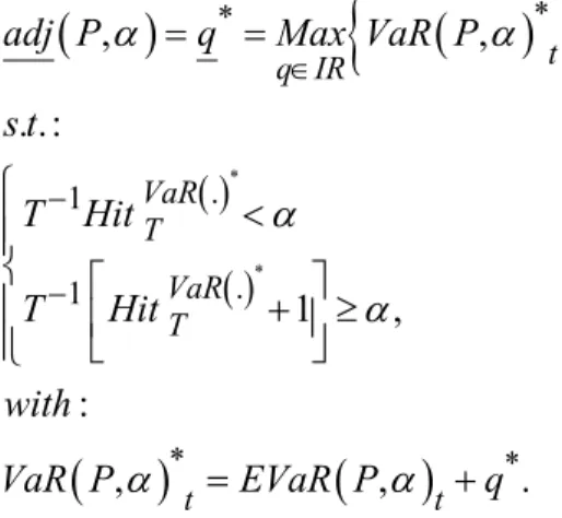
In other words, since the estimated VaR and the bounding range are known, we now have to search, amongst all possibilities, for the minimum (unconditional) adjustment that allows us to recover a corrected estimated VaR that respects condition (4) over the whole sample, i.e.:
(
)
{
(
)
}
( ) ( )(
)
(
)
* * * * . 1 . 1 * * , , . .: 1 , : , , . t q IR VaR T VaR T t tadj P q Max VaR P
s t T Hit T Hit with VaR P EVaR P q a a a a a a Î -= = ì < ïï í é ù ï ê + ³ú ï ë û î = + (5)
Figure 1 represents the minimum adjustments (absolute errors) to be applied to the estimated VaR, denoted q* as solutions of the (static) optimization program (5), for a one-year Historical-simulated VaR computed on the DJIA over more than one century (from the 1st January, 1900 to the 13th September, 2011). Three VaR methods are considered: the
“popular” Historical-simulated approach (Panel A), the parametric Normal approach (panel B) and the semi-parametric RiskMetrics model developed by JP Morgan (Panel C).
These adjustments thus represent the minimal global constants that we should have added to the quantile estimations for having reached a VaR sequence that does not reject the null hypothesis of the Hit test (no difference between theoretical and empirical probabilities of VaR violations) over the whole sample, at the considered levels of confidence. We observe that the Historicalsimulated error is quite significant for all quantiles (between 0.5% and -7% in absolute terms, i.e. 15% or so in relative terms) and that the 5-95% confidence bounding range is small (some basis points in general). The error significantly increases (in absolute terms) with the confidence level, even when we have the full knowledge of one century of quotes13. The average annualized VaR appear much more aggressive based on the
parametric Normal and the RiskMetrics methods, such as the minimal corrections (adjustments), are more important with these two methods.
Figure 1
Average Annualized VaR
and Associated Minimum Model Risk Adjustments for 250 days
Average Annualized VaR Adjustment in Absolute Value
Panel A: Historical-simulated VaR
-55.00% -50.00% -45.00% -40.00% -35.00% -30.00% -25.00% -20.00% 95.0% 95.5% 96.0% 96.5% 97.0% 97.5% 98.0% 98.5% 99.0% 99.5%
Panel B: Normal VaR
-45.00% -40.00% -35.00% -30.00% -25.00% -20.00% 95.0% 95.5% 96.0% 96.5% 97.0% 97.5% 98.0% 98.5% 99.0% 99.5%
Panel C: RiskMetrics VaR
-45.00% -40.00% -35.00% -30.00% -25.00% -20.00% 95.0% 95.5% 96.0% 96.5% 97.0% 97.5% 98.0% 98.5% 99.0% 99.5%
Source: Bloomberg; daily data of the DJIA index in USD from the 1st January, 1900 to the 13th September, 2011. The first plot (on the left hand
side) represents the non-adjusted average annualized VaR level. The minimal adjustment is represented in the second plot and is expressed in absolute value (on the right hand side). The minimal adjustment necessary to respect the hit ratio criterion is here considered as a proxy of the economic value of the model risk. The Historical, Normal and RiskMetrics VaR are computed on a daily horizon as an annualized empirical quantile using 250 days of past returns. Without any adjustment, the imperfect Estimated VaR is underestimated (too permissive) in each of these cases. The adjustments are calculated on the entire VaR forecast sample. The aim is to see here if, when we have the maximum information possible (a century of quotes or so), we still face model risks. The standard-errors are computed based on a block-bootstrap method with windows of ten years of daily returns. Computations by the authors.
-6.00% -5.00% -4.00% -3.00% -2.00% -1.00% 0.00% 1.00% 95.0% 95.5% 96.0% 96.5% 97.0% 97.5% 98.0% 98.5% 99.0% 99.5% Minimal Adjustment (250 days) +/- 2 Standard Errors
-16.00% -14.00% -12.00% -10.00% -8.00% -6.00% -4.00% -2.00% 0.00% 2.00% 95.0% 95.5% 96.0% 96.5% 97.0% 97.5% 98.0% 98.5% 99.0% 99.5% Minimal Adjustment (250 days) +/- 2 Standard Errors
-12.00% -10.00% -8.00% -6.00% -4.00% -2.00% 0.00% 95.0% 95.5% 96.0% 96.5% 97.0% 97.5% 98.0% 98.5% 99.0% 99.5% Minimal Adjustment (250 days) +/- 2 Standard Errors
4. Model Risk, Horizon and Long-term Asset Allocations
We evaluate hereafter the term-structure of model risk on VaR estimates varying the length of periods of interest and then focus on its impact on optimal portfolios, integrating risk budgeting at various time horizons.
A Term-structure of Model Risk
In this sub-section, VaR is used for quantifying the risk associated to asset allocations that differ according to their component weights. We first aim to measure required adjustments for the several considered horizons. The data correspond to the daily Dow Jones Industrial Average index (DJIA, total return in USD) from the 1st January, 1900 to the 13th
September, 2011. Figure 2
An Illustration of some Artificial DJIA-based Series
01/00 12/09 12/19 11/29 11/39 11/49 10/59 10/69 09/79 09/89 08/99 08/09 101 102 103 104 105 Original Series Simulated Series
Source: Bloomberg; daily data of the DJIA index in USD from the 1st January, 1900 to the 13th September,
2011. The figure plots the semi-logarithm prices of the original DJIA series and the simulated series. The simulated series are computed by the surrogate data method (Schreiber, 1998) for creating 100 artificial realistic long-term series (randomly chosen amongst the 30,000 created and used hereafter). Computations by the authors.
In order to compute plausible long-term VaR, we use the surrogate data method (Schreiber, 1998) for creating artificial realistic long-term series. This method explicitly allows us to keep some specified time-patterns for returns along a process of a constrained randomization. More precisely, the algorithm is basically based on a re-shuffling of the original return data, with at each step a test of the new generated series, relying on some constraints. After each series of random pairwise updates, some characteristics of the new (resampled) data are computed and it is accepted, if there is no large difference in the parameters compared to the original return series ones14. Figure 2 illustrates a group of 100
random series (out of the 30,000 created and used hereafter).
The minimum adjustments (error terms in absolute values) for various time horizons on the pseudo-DJIA series are represented in Figure 3. The adjustments represent the minimum surplus of VaR that we should have added to empirical VaR for not being blamed by the regulators according to the traffic light control. Three VaR estimating approaches are considered: the Historical-simulated (Panel A), the parametric Normal (Panel B) and the RiskMetrics (Panel C) methods. Adjustment terms associated to VaR represented in this figure are annualized and determined depending on the horizons from 1 to 50 years.
The negative correction implies that VaR should have been more prudent than they were when model risk was not integrated. The magnitude of model risk is inferior to 4% in absolute terms for the Historical-simulated and Gaussian VaR. We observe a non-linear relationship between the corrections on VaR estimates (on the three estimates, namely Historical, Gaussian and RiskMetrics) and the horizon considered, with a special inverse U-shaped relation for the Historical-simulated VaR (whatever the confidence level considered). Model risk of the Historical-simulated VaR is larger for short (below 5 years) and long-term horizons (superior to 40 years), than for mid-term horizons (10-40 years). On the contrary, the minimal adjustment associated to the Normal VaR is near zero at long-term horizons. With
the RiskMetrics Model, while the adjustment appears positive for mid-term and long-term horizons (too conservative VaR), at a 6-year horizon, the correction is quite large15. The
intuition at this stage is that model risk may have strong consequences on asset allocations since the horizon as well as the method for VaR computations have their importance.
Impact on Long-term Asset Allocations
Generally speaking, long-term investors face a dilemma in bad market conditions: ceteris paribus, when prices fall, one may guess that relative valuations might be better in the long run (specifically for long-term horizons) since prices move from a lower level; this makes stocks more attractive in the short-term. However, if the weight in the risky asset is reinforced, risk increases and potential losses might be more severe in the short-term.
Short-term and long-term arguments for reducing or increasing risk are here opposed. A safety first criterion16, which focuses on loss probabilities, may help the investor to solve
the problem, imposing a limit on some long-term positive reasoning. However, uncertainty on risk measures might also be at stake.
From a theoretical point of view, asset allocations integrating risk budgeting (safety first criteria) can both be explained within the maximization of the expected utility framework (Basak, 1995 and 2002) or within the so-called Prospect Theory of Kahneman and Tversky (1979) with a loss-averse agent (Berkelaar et al., 2004; Gomes, 2005). An insured portfolio is thus optimal when the investor has a decreasing risk aversion (Kingston, 1989).
Figure 3
Term-structure of Historical-simulated One to Fifty-year VaR Models for level 99.5% Panel A: Historical-simulated VaR
Panel B: Normal VaR
Panel C: RiskMetrics VaR
Source: Bloomberg; daily data of the DJIA index in USD from the 1st January, 1900 to the 13th September, 2011.
The minimal adjustment, (in absolute value) necessary to respect the Hit ratio criteria, is considered as a proxy of the economical value of the model risk and here is static and annualized. The Historical, Normal and RiskMetrics VaR are computed on various horizons (from 1 to 50 years), as an empirical quantile on a rolling time-window of 1,305 past returns (the whole sample, corresponding to the maximum information). The adjustment terms associated with the Historical VaR presented in this Figure are calculated with respect to time horizons, then annualized, and finally smoothed according to a third-degree polynomial adjustment from 1 to 50 years. The standard-errors are computed based on a block-bootstrap method with windows of ten years of daily returns. Computations by the authors
-6% -5% -4% -3% -2% -1% 0% 1% 2% 0 5 10 15 20 25 30 35 40 45 50
Minimal Adjustment +/- 2 Standard Errors
-7% -6% -5% -4% -3% -2% -1% 0% 1% 2% 0 5 10 15 20 25 30 35 40 45 50
Minimal Adjustment +/- 2 Standard Errors
-20% -15% -10% -5% 0% 5% 10% 0 5 10 15 20 25 30 35 40 45 50
The link between the risk aversion and guaranteed portfolio is thus clearly established and will be addressed hereafter.
Let us suppose that we are at time T and we want to write the portfolio optimization program corresponding to an investor who buys and holds some assets until the horizon H. In order to simplify the theoretical relation without loss of generality, we first, hereafter, suppose that there are only two assets in the market (a risky and a riskless one)17 and that the real
interest rate served on the riskless asset is constant and equals to rf. If we note WT =1 as the
initial wealth and ω the weight in the risky asset, the wealth of the agent at horizon H reads: WT H+ = -(1 ω)exp(r Hf )+ωexp(r H rf + T+1+ +K rT H+ ). (6)
Moreover, let us suppose that preferences of the investor are well described by a power utility function such as:
v W( ) 1= -
(
γ W)
1-γ,(7) where γ is the risk aversion coefficient.
We can write the cumulated excess return on the risky asset on period H as such:
RT H+ =rT+1+rT+2 + +L rT H+ . (8)
The investor who follows a buy-and-hold strategy would adopt an optimal asset allocation that is a solution of the following optimization program (Barberis, 2000):
1 (1 )exp( ) ( ) , 1 γ f f T H T ω IR ω r H ω r H R ArgMax E γ + -+ Î ìé - + + ù ü ïë û ï í - ý ï ï î þ (9) under the following constraints:
(
)
min ( )0 1 ( ),
VaR loss constraint
budget constraint T H W W a w + ³ ì í £ £ î
where ET(.) is the conditional expectation at time T, VaR (α WT H+ ) the maximum potential loss
at a threshold α for an horizon H, and Wmin the minimum capital reserve (corresponding to the targeted pseudo-guarantee at the horizon H).
Figure 4 represents asset allocations for various horizons (from 1 to 50 years), as well as the ratio of minimum adjustment for model risk (between VaR with or partially without model risk) corresponding to the same horizon. We consider three main asset classes: Equities, Bonds and Money market products. Equities have a high risk and return on the global sample, whilst bonds have moderate risk and return and cash is riskless in nominal terms. In reality, cash is exposed to a modest inflation risk (during the so-called “Great Moderation” period), but it is conventional to ignore this to simplify the analysis in short-term analyses. However, long-term investors face a common problem: how to maintain the purchasing power of their assets over time and achieve a level of real returns consistent with their investment objectives? Thus, we herein consider real returns18 in optimal allocation
exercises. On the left y-axis in Figure 4, safety first optimal weights for each asset class are represented (maximization of the expected return under a criterion of VaR at 99.5%), whilst the right y-axis reports the level of the ratio of the required adjustment versus the raw empirical VaR on the corresponding relevant horizons. We use here data extracted from Datastream from 30th March, 1973 to the 13th September, 2011. 19
Figure 4
Time-horizon Safety First Allocations in the Main Asset Classes and Historical VaR Errors
Source: DataStream; daily data from the 30th March, 1973 to the 13th September, 2011. The asset
allocation scale is reported on the left axis and the model risk adjustment relative to the estimated VaR without correction (bold curve) is located on the right axis. The asset allocation consists of a maximization, for each time horizon (50, 49,…, 1), of the agent utility function for a risk aversion coefficient set to 0 (aggressive agent) under a 99.5% VaR constraint of being positive at the specified horizon. We here use 30,000 simulated surrogate real series, built with the historical daily series of 1973-2011, for generating returns considered here on each horizon. Computations by the authors.
This figure indicates that, for long-term horizons, VaRs are considerably under-estimated and the ratio of the correction term out of the uncorrected VaR expands exponentially with the investment horizon. This correction ratio reaches 100% for the 50-year horizon in our simulations, which indicates that the extreme loss is twice the one considered when model risk is ignored, leading to an asset allocation with a very different extreme risk.
Table 2
Optimal Long-only Asset Allocation Weights in Stocks according to a Safety First Guarantee Level and an Horizon
Surrogate simulated series
Horizons (in years)
Levels of Targeted Minimum Return 35 30 25 20 15 10 5 Panel A: 95% VaR Optimal Weight 100.00% 100.00% 100.00% 100.00% 84.06% 66.44% 24.26% 0% Over-weight 0.00% 0.00% 0.00% 0.00% 9.24% 5.72% 2.87% Optimal Weight 100.00% 100.00% 100.00% 100.00% 100.00% 82.61% 49.70% 1% Over-weight 0.00% 0.00% 0.00% 0.00% 0.00% 10.08% 8.71% Optimal Weight 100.00% 100.00% 100.00% 87.46% 71.46% 52.54% 18.55% 2% Over-weight 0.00% 0.00% 0.00% 0.00% 3.80% 5.54% 3.33% Panel B: 99.5% VaR Panel B : VaR 99,5% Optimal Weight 97.73% 92.46% 85.99% 77.16% 64.30% 46.47% 23.00% 0% Over-weight 3.97% 3.19% 5.23% 7.34% 6.78% 3.86% 1.94% Optimal Weight 88.76% 82.50% 73.94% 63.48% 50.80% 30.52% 16.14% 1% Over-weight 2.41% 3.51% 4.71% 6.58% 6.54% 3.20% 1.21% Optimal Weight 75.15% 65.67% 57.37% 44.28% 29.31% 15.12% 8.34% 2% Over-weight 1.43% 2.41% 2.24% 4.61% 4.33% 2.52% 2.25%
Source: Datastream and Bloomberg, weekly NAV in EUR from the period 30th March, 1973 to the 13th September,
2011. This table presents (non adjusted for model risk) optimal allocations in stocks as well as the over-weight computed such that the difference between the non-adjusted optimal weight and the model risk adjusted optimal weight, for various targeted VaR (0%, 1%, 2% at horizon), horizons (from 5 to 35 years) and two confidence levels (95% in panel A and 99.5% in Panel B). We also calculated the optimal weights for the horizons from 35 to 50 years; we obtain the same orders of magnitude for the over-weight variations. We here use 30,000 simulated surrogate real series, built with the historical daily series of 1973-2011, for generating returns considered here on each horizon. Computations by the authors.
Table 2 focuses on the optimal weights in equities when considering, or not, adjusted VaR for model risk. This table presents (non-adjusted for model risk) optimal allocations in equities, as well as the over-weight computed as the difference between the non-adjusted optimal weight and the model risk adjusted optimal weight, for various targeted period VaR of real returns (0%, 1%, 2%), horizons (from 5 to 35 years) and two confidence levels (95% in panel A and 99.5% in Panel B). This table shows that given the other characteristics of stocks (in terms of performance and volatility), the model risk effect on the “equity” class in the optimal portfolios is more limited at very long-term horizons but significant up to 25
5. Conclusion
In this paper, we first illustrate and estimate the model risk of risk models (see also Boucher et al., 2012a) and we evaluate its impact on long-term asset allocations. Firstly, we evaluate the simple effect of estimation and specification risks on VaR estimates. Secondly, we propose a general method to compute risk measures robust to the main model risks. Thirdly, we then evaluate the impact of corrected VaR estimates on the optimal asset allocations, integrating risk budgeting, at various time horizons
Based on a US database, we find that model risk is widely neglected by the main risk models in asset allocation exercises. Our results suggest a non-linear relationship between the corrections on VaR estimates and the horizon considered. This non-linear relation exhibits an inverse U-shaped pattern for the Historical-simulated VaR (whatever the confidence level considered). In the case of the mainstream risk model (Historical-simulated VaR), model risk is thus larger for short (below 5 years) and long-term horizons (superior to 40 years) than for mid-term horizons (10-40 years).
Moreover, based on the optimal adjustment procedure to obtain a sequence of VaR that allows us to go through the validation tests of market authorities, we show that the long-term asset allocation (for the main asset classes on the European market) is significantly modified. The “equity” class in optimal portfolios is indeed reduced on all the given horizons up to 25 years. Our results suggest that stocks are less appealing to long-horizon investors when considering the risk model of model risks than conventional wisdom would suggest, when no model risk is considered.
The same metric – the size of the required buffer – could be used to gauge the relevance of any proven model (amongst theoretically justified models) and allow the risk manager to compare them on that basis. However, it would be worthy of interest to study
more extensively the model risk of the proposed model risk correction (see Boucher et al., 2012b).
The next steps in our research agenda will consist, first, in investigating the differences in the suggested correction for model risk in terms of level and dynamics for different types of assets (including real estate, commodities and other diversifying vectors of investments) and countries/regions in an international perspective. Secondly, we have to further examine the kind of processes (stability, breaks, jumps, persistence, etc.) followed by the model risk correction in link with the global macro-financial environment. Thirdly, we should be able to consider other valuable properties of VaR (such as the size and dependence of exceptions and not only their frequency) when we calibrate model risk correction (see Boucher et al., 2012b). Finally, investigating asset-allocation decisions, while including model uncertainty about both risks and expected returns, would also offer an interesting direction for future researches.
References
Aït-Sahalia Yacine, Julio Cacho-Diaz and Roger J. Laeven, “Modeling Financial Contagion using Mutually Exciting Jump Processes”, Princeton Working Paper (2012):43 pages. Alexander Carol and José M. Sarabia,“Quantile Uncertainty and Value-at-Risk Model Risk”,
Risk Analysis 32 (2012):1293-1308.
Applebaum David, “Lévy Processes - From Probability to Finance and Quantum Groups”, Notices of the American Mathematical Society 51(2004):1336-1347.
Barberis Nicals, “Investing for the Long Run when Returns are Predictable”, Journal of Finance 55 (2000):225-264.
Basak Suleyman, “A General Equilibrium Model of Portfolio Insurance”, Review of Financial Studies 8(1995):1059-1090.
Basak Suleyman, “A Comparative Study of Portfolio Insurance”, Journal of Economic Dynamics and Control 26 (2002):1217-1241.
Basel Committee on Banking Supervision, International Convergence of Capital Measurement and Capital Standard, Bank for International Settlements (1988):30 pages. Basel Committee on Banking Supervision, Amendment to the Capital Accord to Incorporate
Basel Committee on Banking Supervision, Revisions to the Basel II Market Risk Framework, Bank for International Settlements (2009):35 pages.
Berkelaar A., R. Kouwenberg and T. Post, “Optimal Portfolio Choice under Loss Aversion”, Review of Economics and Statistics 86 (2004):973-987.
Berkowitz Jeremy and James O’Brien, “How Accurate are Value-at-Risk Models at Commercial Banks?”, Journal of Finance 57 (2002):1093-1111.
Boucher Christophe and Bertrand Maillet, “The Riskiness of Risk Models”, mimeo (2012a):10 pages.
Boucher Christophe, Jón Daníelsson, Patrick Kouontchou and Bertrand Maillet, “Risk Model-at-Risk”, mimeo (2012b):47 pages.
Christoffersen Peter F., “Evaluating Interval Forecasts”, International Economic Review 39 (1998):841-862.
Christoffersen Peter F. and Sílvia Gonçalves, “Estimation Risk in Financial Risk Management”, Journal of Risk 7 (2005):1-28.
Christoffersen Peter F., Value-at-Risk Models, Part 5 in Handbook of Financial Time Series, Andersen-Davis-Kreiss-Mikosch (Eds), Springer-Verlag (2009):753-766.
Cont Rama, “Model Uncertainty and its Impact on the Pricing of Derivative Instruments”, Mathematical Finance 16 (2006):519-547.
Efron Bradley and Robert Tibshirani, An Introduction to the Bootstrap, Cox-Hinkley-Reid-Rubin-Silverman (Eds), Chapman & Hall/CRC, New York, (1994):456 pages.
Gizycki Marianne and Neil Hereford, “Assessing the Dispersion in Banks’ Estimates of Market Risk: The Results of a Value-at-Risk Survey”, Discussion Paper 1, Australian Prudential Regulation Authority (1998):37 pages.
Gouriéroux Christian and Jean-Michel Zakoïan, “Estimation Adjusted VaR”, Econometric Theory, forthcoming (2012):42 pages.
Gomes Francisco J., “Portfolio Choice and Trading Volume with Loss-averse Investors”, Journal of Business 78 (2005):675-706.
Jorion Philippe, “Risk Management Lessons from the Credit Crisis”, European Financial Management 15 (2009):923-933.
Kahneman Daniel and Amos Tversky, “Prospect Theory: An Analysis of Decision under Risk”, Econometrica 47 (1979):263-291.
Kerkhof Jeroen, Bertrand Melenberg and Hans Schumacher, “Model Risk and Capital Reserves”, Journal of Banking and Finance 34 (2010):267-279.
Kingston Geoffrey, “Theoretical Foundations of Constant Proportion Portfolio Insurance”, Economics Letters 29 (1989):345-347.
Kupiec PAUL H., “Techniques for verifying the Accuracy of Risk Measurement Models”,
Journal of Derivatives 3 (1995):73-84.
Levy Haim and Moshe Levy, “The Safety First Expected Utility Model: Experimental Evidence and Economic Implications”, Journal of Banking and Finance 33 (2009):1494-1506.
Monfort Alain., “Optimal Portfolio Allocation under Asset and Surplus VaR Constraints”, Journal of Asset Management 9 (2008):178-192.
Pástor Lubos and Robert F. Stambaugh, “Are Stocks Really Less Volatile in the Long Run?”, Journal of Finance 67 (2012):431-478.
Pérignon Christophe, Zi Y. Deng and Zhi J. Wang, “Do Banks overstate their Value-at-Risk?”, Journal of Banking and Finance 32 (2008):783-794.
Pérignon Christophe and Daniel R. Smith, “The Level and Quality of Value-at-Risk Disclosure by Commercial Banks”, Journal of Banking and Finance 34 (2010):362-377. Politis Dimotris N. and Joseph P. Romano, “The Stationary Bootstrap”, Journal of the
Schreiber Thomas, “Constrained Randomization of Time Series Data”, Physical Review Letters 80 (1998):2105-2108.
Sharma Meera, (2012), “The Historical Simulation Method for Value-at-Risk: A Research Based Evaluation of the Industry Favourite”, Working Paper Indian Institute of Management (2012):22 pages.
Stahl Gerhard, “Three Cheers”, Risk Magazine 10 (1997):67-69.
Notes
1 For example, JP Chase reported 5, Credit Suisse 7 and UBS 16 exceedances based on the 1% VaR for a one
day forecasting horizon in Q3 - 2007, which requires a maximum of .63 exceedance given the probability level of 1% (Jorion, 2009).
2 The risk estimates of these models are used to determine capital requirements and associated capital costs of
financial institutions, depending in part on the ex post quality of the recent VaR forecasts.
3 Focusing on the uncertainty about how to model the predictive distribution of future asset returns.
4 Only a few recent papers (e.g. Kerkhof et al., 2010; Gouriéroux and Zakoïan, 2012; Alexander and Sarabia,
2012) yet aim to take model risk into account in the computation of risk measures.
5 In July 2009, the Basel Committee on Banking Supervision issued a directive (“Revisions to the Basel II
Market Risk Framework”) requiring that financial institutions quantify model risk. The Committee further stated that two types of risks should be taken into account: “the model risk associated with using a possibly incorrect valuation, and the risk associated with using unobservable calibration parameters”. The resulting adjustments must impact Tier I regulatory capital, and the directive was to be implemented by the end of 2010.
6 These two sources of error are neither exclusive nor exhaustive. Granularity errors, measurement errors and
liquidity risk are also at the origin of model errors (see, e.g. Boucher et al., 2012b).
7 Using the Chebyshev inequality, Stahl (1997) showed that a multiplier of 3 is reasonable to account for a part
of the model risk. Indeed, the Chebyshev inequality can be transformed to a VaR inequality where a prudent daily VaR (null averaged return) can be expressed as a multiple of a daily parametric-Gaussian VaR, with a multiple of 2.71 at the 5% level and 4.29 at the 1% level. Note that, based on the Cantelli inequality (the one-sided variant of the Chebyshev inequality), these multiples are respectively equal to 2.64 and 4.27. However, these inequalities transform a specification risk (on the distribution of returns) into an estimation risk (on the standard deviation of returns).
8 The regulatory suggestion is to use (at least) 250 days (BCBS, 1996).
9 See Applebaum (2004) and Aït-Sahalia et al. (2012) for Lévy and Hawkes process definitions.
10 The relative error of 30% corresponds to the probability of 99.90% with a window of 250 days for the Lévy
DGP (i.e. -22.74 out of -73.74).
11 Note that the model uncertainty problem becomes even more severe in a continuous-time world or with
intraday data where jumps occur quite often. However, in this paper we focus on crucial consequences of such model risk on asset allocation, so that the daily frequency is the highest frequency considered in our analyses.
12 Note that, if we assume that the exceptions or hits are Independently and Identically Distributed then, under
the unconditional coverage hypothesis (Kupiec, 1995), the total number of VaR exceptions (cumulated hits) follows a binomial distribution (Christoffersen, 1998).
13 Besides this, complementary tests (on 500 and 750 sample days, see Appendix – Figures A1 and A2) show
that the smaller the estimation period, the more important the (dynamic) adjustment (both in absolute and relative terms) for the historical method. This phenomenon can be explained by the fact that using larger estimation periods more likely leads to taking into consideration extreme realizations and crisis episodes.
14 In our case: the first four moments, the first autocorrelation coefficient on returns, the first significant squared
return autocorrelation coefficient, the freedom parameter of a t-student, the number of breaks, the long memory coefficient and the mean-reverting index, are all tested, and the new series is accepted if the quadratic relative difference in parameters is inferior to 10%.
15 The shape of these corrections is similar for other confidence levels of VaR (see Appendix – Figures A3 and
A4).
16 The safety first criterion advocates the minimization of the probability of outcomes below a certain ‘‘disaster”
level (e.g. Levy and Levy, 2009).
17 This relation can be extended to several assets with no difficulties.
18 with a linear interpolation of the monthly Consumer Price Index to compute a daily price index.
19 The “Equity” asset class is represented by a composite index of 95% of the MSCI Europe + 5% MSCI World;
ALL MATS index (when available) and for the “Money Market”, the BUNDESBANK INTEREST RATE index and the EURO OVERNIGHT INDEX AVERAGE index (when available).
20 Note that these results remain qualitatively the same when a short-sale constraint is no longer considered.
Moreover, these results are robust to various simulations and optimization programs (both results are available upon request).