Adaptive transmit beamforming for simultaneous transmit and receive

Adaptive Transmit Beamforming for Simultaneous

Transmit and Receive

by

Daniel L. Gerber

B.S., Massachusetts Institute of Technology (2010)

Submitted to the

Department of Electrical Engineering and Computer Science

in partial fulfillment of the requirements for the degree of

Master of Engineering in Electrical Engineering and

Computer Science

at the

MASSACHUSETTS INSTITUTE OF TECHNOLOGY

MASSACHUSETTS INSTMLITE OF TECHNOLOGY

JUN 2

1

2011

LIBRARIES

ARCHNES

June 2011

@

Massachusetts Institute of Technology 2011. All rights reserved.

A u th or ... V . .

...

Department of Electrical Engineering and Computer Science

April 28, 2011

Paul D. Fiore

Sta

ember, MIT Lincoln Laboratory

3eRimtrvisor

Certified by...

David H. Staelin

Professor of Electrical Engineering and Computer Science

Thesis Supervisor

Accepted by...

_...

_{... .D...}

\- "Dr. Christopher J. Terman

Chairman, Department Committee on Graduate Theses

Adaptive Transmit Beamforming for Simultaneous Transmit

and Receive

by

Daniel L. Gerber

Submitted to the Department of Electrical Engineering and Computer Science on April 28, 2011, in partial fulfillment of the

requirements for the degree of

Master of Engineering in Electrical Engineering and Computer Science

Abstract

Simultaneous transmit and receive (STAR) is an important problem in the field of communications. Engineers have researched many different models and strategies that attempt to solve this problem. One such strategy is to place a transmit-side null at the receiver in order to decouple a system's transmitter and receiver, thus allowing them to operate simultaneously. This thesis discusses the use of gradient based adaptive algorithms to allow for transmit beamforming. Several such algorithms are devised, simulated, and compared in performance. Of these, the best is chosen to study in further detail. A mathematical analysis is performed on this particular algorithm to determine a linearized state space model, which is then used in a noise analysis. An important benefit of these algorithms is that they do not require computationally intensive matrix operations such as inversion or eigen-decomposition. This thesis ultimately provides, explains, and analyzes a viable method that can form a transmit-side null at the receiver and extract a weak signal of interest from the received signal while simultaneously transmitting another signal at high power.

Thesis Supervisor: Paul D. Fiore

Title: Staff Member, MIT Lincoln Laboratory

Thesis Supervisor: David H. Staelin

Acknowledgements

First and foremost, I would like to thank my direct supervisor Paul Fiore. This thesis would not have been possible without the constant support Paul gave me through meetings, mathematical discussion, and ideas. I would also like to thank Jeff Herd for his support in organizing and leading the members working on the STAR project at Lincoln Laboratory. Thanks also to Dan Bliss who put me up to date with current research in the field of STAR. In addition, I would like to thank my MIT thesis adviser David Staelin and MIT academic adviser David Perreault for supporting me in my master's degree. Finally, I would like to thank my family and friends, who have

Contents

1 Introduction 8

2 Background Theory 13

2.1 Control Theory . . . . 13

2.2 Gradient Descent and Numerical Methods . . . . 16

2.3 Adaptive Linear Combiner . . . . 18

2.4 Least Mean Squares Algorithm . . . . 20

2.5 Normalized LMS Algorithm . . . . 22

2.6 Applications of the LMS Algorithm . . . . 23

2.7 Signal Orthogonality . . . . 27

2.8 Receive Adaptive Beamforming . . . . 30

2.9 Transmit Adaptive Beamforming . . . . 35

3 Methods and Algorithms for Multiple-Input Single-Output (MISO) Active Cancellation ₃₉ 3.1 Transmit Beamforming Method: Trial and Error . . . . 41

3.2 System Identification for Channel Estimation . . . . 46

3.3 Transmit Beamforming Method: Gradient Descent . . . . 49

3.4 Transmit Beamforming Method: Trial and Error Using a Channel Es-tim ate . . . . 54

Channel Estimation Method: Probing Duty Cycle . . . . Channel Estimation Method: Orthogonality-Based Probing Scheme . Extracting the Signal of Interest . . . .

4 Mathematical Analysis of the Trial and Error with a mate Method

4.1 Linearized System Dynamics . . . . 4.2 System Response to an Input . . . . 4.3 Analysis of Noise on the System Input . . . .

Channel

Esti-5 Conclusion

A Source Code

A.1 Matlab Code for Trial and Error Method . . . . A.2 Matlab Code for Gradient Descent Method . . . . A.3 Matlab Code for Trial and Error Method with a Channel Estimate.

A.4 Matlab Code for Probing Duty Cycle Method . . . .

A.5 Matlab Code for Orthogonality Based Probing Method . . . . A.6 Matlab Code for Noise Variance Simulation . . . .

Bibliography 3.6 3.7 3.8 96 98 98 101 104 108 112 118 121

List of Figures

1-1 STAR Block Diagram ... ...

2-1 State Space Block Diagram . . . .

2-2 Adaptive Linear Combiner . . . .

2-3 Parallel LMS Configuration . . . ....

2-4 Traversal LMS Configuration . . . . 2-5 System Identification LMS Filter . . . . 2-6 Adaptive Interference Cancellation LMS Filter 2-7 Two-Antenna Receive Beamforming Canceller 2-8 Traversal Adaptive Filter Array . . . .

3-1 3-2 3-3 3-4 3-5 3-6 3-7 3-8 3-9 3-10

Transmitter Filter Block Diagram Trial and Error Timing Diagram. Trial and Error Flow Chart . . Trial and Error Received Power Trial and Error Weights . . . . Trial and Error Channel . . . . Channel Estimate Block Diagram Gradient Descent Received Power Gradient Descent Weights... Gradient Descent Received Power 2

. . . . 42 . . . . 42 . . . . 42 . . . . 44 . . . . 44 . . . . 45 . . . . 46 . . . . 52 . . . . 52 . . . . 53

3-11 Trial Error Channel Estimate Received Power

Trial Error Channel Estimate Weights . Trial Error Channel Estimate Weights Zoo Trial Error Channel Estimate Received Po

3-15 Trial Error Channel Estimate Weights 2

Probe Signal Block Diagram . . . . Probing Duty Cycle Timing Diagram Probing Duty Cycle Received Power Probing Duty Cycle Received Power 2 Probing Duty Cycle Weights . . . . Probing Duty Cycle Weights 2 . . . . Orthogonality Based Probing Received Pc Orthogonality Based Probing Weights . . Orthogonality Based Probing Weights 2. Signal of Interest Block Diagram . . . .

Signal of Interest . . . . Signal of Interest Received Power . . . .

4-1 Noise Analysis Simulation

3-12 3-13 3-14 . . . . 5 6 m ed . . . . 57 wer 2 . . . . 58 . . . . 5 8 . . . . 6 0 . . . . 6 1 . . . . 6 2 . . . . 6 2 . . . . 6 3 . . . . 6 3 )wer . . . . 68 . . . . 6 8 . . . . 6 9 . . . . 7 2 . . . . 7 2 . . . . 7 3 . . . . . 95 3-16 3-17 3-18 3-19 3-20 3-21 3-22 3-23 3-24 3-25 3-26 3-27

. .. . . .

56

Chapter 1

Introduction

The simultaneous transmission and reception (STAR) of signals on the same frequency band is an important engineering challenge that still has not been adequately solved. Past attempts have included isolation methods between the transmitter and receiver

[1, p. 16]. However, such methods offer minimal improvement in cancellation of the

high power transmit signal at the receiver. Antenna isolation can provide a 30dB drop in transmit signal power at the receiver. An additional 30dB drop can result if the transmitter and receiver are cross-polarized with respect to one another [1, p. 18] Another technique under investigation is that of active STAR. Active STAR in-volves the use of feed-forward electronics and algorithms to use the transmit signal as an input to the receive control loop. The transmit signal is filtered before it is sub-tracted from the received signal. As a final result, the transmit signal is cancelled from the received signal and the receiver can now detect other external signals of interest

(SOI). In addition, the transmitter will not saturate or damage the analog-to-digital

converters (ADC) on the receiver.

Active cancellation greatly improves the system performance at a level comparable to passive techniques [1, p. 20]. In addition, the techniques for active and passive cancellation all complement each other in reducing the amount of transmitted signal

at the receiver. For example, an RF canceller can lower the transmit signals' power

by up to 35dB [2, p. 8]. With another 60dB of well engineered antenna isolation and

cross-polarization, the transmit power at the receiver will be 95dB lower.

One cancellation technique that can be applied in any sort of STAR or full duplex design is the use of multiple input multiple output (MIMO) antenna systems. The MIMO antenna array is very important for interference cancellation and isolation. Single input single output (SISO) antenna isolation techniques include polarizing the transmit and receive antennae in different planes, pointing them in different directions, distancing them, or shielding them from each other. The MIMO system can utilize these SISO cancellation techniques, but can also be set up such that the transmit beampattern places a null at the receive antenna location. In general, null points exist in systems with multiple transmitters because the transmitted signals have regions of destructive interference.

An early proposal [3] discusses interference cancellation for use in STAR. That paper proposed an interference cancellation LMS filter (treated here in Section 2.6) to cancel the transmitted signal from the receiver, after which experiments are performed on such a system. Previous work in wideband interference cancellation was performed in [4], in which several methods were tested in Matlab to compare performance and computational complexity. Experiments were performed in [1] to investigate various strategies of antenna isolation and interference cancellation for use in SISO STAR. These prior experiments differ from the setup in this thesis, wherein MIMO STAR is used to overcome the challenges of receiver saturation and a time variant channel. A similar idea [5] suggests augmenting the conventional SISO time domain cancellation techniques with MIMO spatial domain techniques. The techniques of zero-forcing and MMSE filtering were investigated and simulated. This thesis does not pursue these techniques in order to avoid the computationally intensive matrix inversion (or pseudo-inverse). In addition, the methods of this thesis deal with unknown

time-variant channel models.

The work of Bliss, Parker, and Margetts [6] is the most relevant to this thesis. Those authors present the general problem of MIMO STAR communication, but focus specifically on the problems of simultaneous links and a full duplex relay. The analysis in their paper assumes a known time-variant channel that can be modeled as a matrix of channel values at certain delays. With knowledge of the signal and received data, the maximum likelihood channel estimate can be derived using the ordinary least squares method. The paper follows by proving that this method maximizes the signal to noise ratio. In addition, it demonstrates the method's performance through simulations of the simultaneous links and the full duplex relay problems. However, like [5], [6] requires matrix inversion. This thesis project is aimed at developing a robust method that does not require computationally intense calculations to solve for optimal weights. In addition, this thesis accounts for a prior lack of channel data and presents methods to probe the channels without saturating the transmitter.

This thesis will explore the digital portion of the STAR system design, with an emphasis on algorithms that make full duplex multipath communication possible in a changing environment. This STAR system's digital portion revolves around a digital MIMO LMS filter, as shown in Figure 1-1. The MIMO LMS filter will help to protect the ADCs from saturation or noisy signals. In addition, it will be able to filter out the transmitted signal from the received signal after the received signal has passed into the digital domain. The LMS filter will be the first step in the system's digital signal processing [2, p. 9].

The remainder of this thesis is organized as follows. A brief summary of the required background theory is given in Chapter 2. In addition, this chapter will discuss the current research and progress in the field of transmit beamforming. Chapter 3 will describe the methods of STAR that have been proposed and tested. For each method, a brief description of the algorithm and mathematical analysis will be provided and

the method results will be discussed. The best method from Chapter 3 will be chosen

and analyzed in Chapter 4. Chapter 4 will provide an in-depth mathematical analysis,

linearization, and system model for the chosen method. Concluding thoughts are

offered in Chapter 5.

Unwanted Tx - Rx

Coupling

Tx

Transmit

Signal

-o

To Rx

Processing

Figure 1-1: Block diagram for the MIT Lincoln Laboratory STAR system proposal

[2]. Although this diagram shows plans for the antennae, analog electronics, and RF

canceller setup, the focus of this thesis is on digital portion of the system that deals

with transmit beamforming. HPA stands for high power amplifier, LNA stands for

low noise amplifier, DAC stands for digital to analog converter, and ADC stands for

analog to digital converter.

Chapter 2

Background Theory

This thesis presents methods for solving the STAR problem with adaptive transmit

beamforming. Knowledge of adaptive beamforming is required in order understand

the mathematical nature of the algorithms presented in Chapters 3 and 4. This

chapter presents the fundamental background theory of adaptive beamforming and

contains equations that will be important to the analysis in later chapters.

2.1

Control Theory

A system response can be determined by the behavior of its state variables, which

describe some type of energy storage within the system. For example, the voltage on a

capacitor is a state space variable in a circuit system. For systems with multiple states,

the entire set of state variables can be expressed as a vector. Systems with multiple

inputs can likewise have their inputs expressed as a vector. The state evolution

equations of a linear time-invariant (LTI) state space system with multiple inputs

can be written as [7, p. 284]

r[n] -+

t$I

~

Z

'

~

Uy[n]

Figure 2-1: Block diagram of a state space system, with input vector r[n], state vector

w[n], and output vector y[n].

where w[n] is a vector containing the state variable at sample time n, r[n] is the

vector of inputs, and A and B are coefficient matrices of the state equation.

State space systems can have multiple outputs with a similar vector notation of

the form

y[n] = Cw[n]+ Dr[n] (2.2)

where y[n] is the output vector. Together, (2.1) and (2.2) form the state space

equations of the system, and can be represented by the block diagram in Figure 2-1.

In the z-domain, these equations can be represented as [8, p. 768]

zw(z) = Aw(z) + Br(z)

y(z) = Cw(z) + Dr(z) . (2.3)

The transfer function from input to state vector is defined as

w(z)

(zI - A)-1

r(z)

and the transfer function from input to output is defined as

y(z) A C(zI - A)-1B + D. _(2.5)

r(z)

We shall define the Resolvent Matrix 4(z) as

4(z) = (zI - A)-1 (2.6)

and note that in the time domain, the State Transition Matrix 4[n] is [7, p. 291]

4[n]

A"

(2.7)

for n > 0. With this information, the state vector becomes [7, p. 289]

w[n]

Anw[O] + 1

A-'Br[m]

(2.8)

m=O

and the system output function is

t

y[n]

CA w[0]+ C I

A"-'Br[m] + Dr[n] .

(2.9)

m=O

Note that the second term of (2.8) is a convolution sum.

To determine the steady state behavior of the state vector w[n], An can be

de-composed into [9, p. 294]

"

=

V-1

where V(A) is the right eigenvector matrix of A and

is the eigenvalue matrix.

Since

is a diagonal matrix, w[n] will converge only if

|Amx,(A)

I<

1, where

is

the

maximum eigenvalue of A.

2.2

Gradient Descent and Numerical Methods

Optimization problems involve tuning a set of variables so that some cost function

is minimized or maximized [10, p. 16]. This function is referred to as the

"perfor-mance surface" and describes the system perfor"perfor-mance with respect to a set of system

variables. In many cases, the performance surface is quadratic, and the local critical

point is the global minimum or maximum [11, p. 21]. Critical points can be found

by determining where the gradient of the performance surface is equal to zero.

Even though an optimal solution to such problems can be mathematically

deter-mined, numerical methods are often useful in practice because they are robust [10,

p. 277]. In this sense, numerical methods are less likely to be affected by practical

difficulties such as modeling errors or poor characterization data.

One particular method of searching the performance surface for local minima is the

gradient descent method. This method starts at some point along the performance

surface, finds the direction of the surface gradient, and steps in the direction of the

(negative) gradient by a small amount [10, p. 277]. In vector form, the gradient of

some function

f

of a vector w is

awi

Vf(w) - - (2.11)

awK

L OWK J

Many numerical methods employ the negative gradient, which often points in the

general direction of a local minimum. By stepping w in this direction every numerical

cycle, the gradient descent method ensures that a local minimum will eventually be

reached if the step size is sufficiently small. Any numerical method that uses gradient

descent will contain an update equation of the form [11, p. 57]

where p is the growth factor. The growth factor determines the step size, which governs the speed and accuracy of the numerical method.

X0

". W

-

- 10

XB

WB

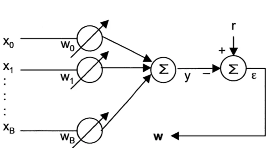
Figure 2-2: Adaptive linear combiner with input x, weights w, and output y.

2.3

Adaptive Linear Combiner

One particular use for gradient descent is in optimizing an adaptive linear combiner, shown in Figure 2-2. Here, the purpose of gradient descent is to minimize the mean squared error (MSE) E[E2

_[n]]

that measurement. Using a gradient descent algorithm, the system error can be fed back into the system input x[n] through the adjustable weight values wk. The rest of this section follows the derivation from [11, p. 19-22]. In the adaptive linear combiner,

E[n]

r[n]

- y[n]

-r-xTw

(2.13)

E2[n] r2[n] - 2r[n]xT[n]w

+

= 2-[n] - 2r[n]xT[n]w + wTx[n]xT[n]w . (2.14)

expectation operator. In other words,

E[E2] = E[r

_{] - 2E[rxT]w}

_E[xx

=

_-2pTw

= E[r2_{] - 2wTp + WT Rw (2.15)}

where R E[xxT] is the input autocorrelation matrix and p = E[rxT] is the

input-to-output crosscorrelation vector.

The gradient of the mean squared error is

VE[E2_]

= E[E2_]

₌

₊

aw

This is the negative of the direction in which a gradient descent algorithm will step on any given cycle of the algorithm. In order to reach the optimal weight value, the algorithm will have to update the gradient every cycle and step in the gradient's direction. Most quadratic performance surfaces such as the MSE have a single global minimum. One exception is the function xTRx in the case that R is low-rank. If we assume that R is of full rank, the optimal weight vector wpt can be found by determining where the gradient is zero. In this case,

0 = -2p + 2Rwopt

wopt = R-1p. (2.17)

The optimal weight vector, also known as the Weiner solution, is the set of weights that positions the system at the bottom of the performance surface and thus minimizes the MSE. In addition, (2.17) is a variation of the Yule-Walker equations [12, p. 410].

2.4

Least Mean Squares Algorithm

The least mean squares (LMS) algorithm is a numerical method that uses gradient descent to minimize the MSE of an adaptive linear combiner. The LMS algorithm uses E2[n] as an unbiased estimate of E[E2

]

E[-2 2[n] = r2_{[n] - 2r[n]xT[n]w + xT [nwxT[n]w (2.18)}

V[n] -2r[n]x[n] + 2x[n]xT[n]w

-2p[n] + 2R[n]w (2.19)

where V[n] is the gradient vector. Note that R[n] and p[n] differ from R and p from Section 2.3 because R[n] and p[n] do not use expected values. One particular consequence of this difference is that R[n] is rank-one because any outer product of the form xxT is rank-one [13, p. 461]. This also causes R[n] to have only one nonzero eigenvalue.

The LMS algorithm uses the gradient descent weight update equation from (2.12). In this case,

w[n + 1]

=w[n] - pV[n]

w[n] + p(2p[n] - 2R[n]w)

(I - 2pR[n])w[n] + 2tp[n] . (2.20)

As shown above, the LMS weight update equation takes on the state space form of (2.1) and (2.2). If the substitutions

A = I - 2LR[n]

B = _2pxT[n]

are made, state space analysis may be used to determine the time response and convergence of the LMS algorithm [14]. The steady state convergence and behavior can therefore be analyzed using (2.8) and (2.10). From (2.8), it follows that

n

w[n] = (I - 2pR[n])"w[0] + Z(I - 2pR[n])n-m(2ptx T [n])r[m] . (2.22)

m=o

Statistical analysis must be used to determine the convergence of the LMS algorithm, since R[n] only has one nonzero eigenvalue. Therefore, we shall use the matrix R =

E[xxT] from Section 2.3 to study the algorithm convergence. Using (2.21), we have

(I

2pR)"

(I

0

<

(2.23)

1Amax,(R)

where V(R) is the right eigenvector matrix of R and A(R) is the eigenvalue matrix. It is easy to see that the weights will not converge if pu is too large.

2.5

Normalized LMS Algorithm

The normalized LMS (NLMS) algorithm replaces the constant p't with a time varying growth factor p[n]. Specifically, [10, p.355]

t[n ] =

x T[n] x[n]

The benefit of normalizing the growth factor with respect to the input is that it causes the gradient to be more resistant to input noise when the amplitude of the input is relatively large [10, p. 352]. Another benefit of the NLMS algorithm is that the stability conditions for [y are constant. As shown in (2.23), the limits on p for the LMS algorithm are relative to Amax,(R), which depends on x[n]. However, for the

NLMS algorithm, [10, p. 355]

2.6

Applications of the LMS Algorithm

In signal processing, the LMS algorithm is used as a filter. The applications of the

LMS filter all differ with how the inputs and outputs are connected. The two basic LMS filter configurations are parallel (the general form) and traversal [11, p. 16].

Figures 2-3 and 2-4 show the difference between the two configurations. The input vector for the parallel configuration is a set of inputs at a particular time. The input vector for the traversal configuration is a set of delayed time samples from a single input. These two LMS filter configurations can be used in a number of applications. There are four basic classes of adaptive filtering applications: system identification, inverse modeling, prediction, and interference cancellation [10, p. 18]. The system identification filter and the interference-cancelling filter are both important to this thesis.

System identification is useful for modeling an unknown system or channel, as shown in Figure 2-5. In the case of the traversal LMS filter, the unknown system is modeled as a set of gains and delays that form a basic finite impulse response (FIR) filter. The LMS filter's weights will adjust themselves to the taps of an FIR filter that best models the unknown system [11, p. 195]. The performance of the algorithm will decrease if there is noise added to the desired signal. Since the LMS filter ideally adjusts its weights to minimize E[E2_{], it is theoretically unaffected by noise if the}

input is uncorrelated to the added noise signal [11, p. 196]. In practice, the noise will affect the system because E2[n] is used in place of E[E2]. The system identification

filter can also potentially fail if the channel of the unknown system is too long. Adaptive interference cancellation attempts to subtract an undesired signal from the signal of interest, as shown in Figure 2-6. This generally requires that the unde-sired signal can be modeled or generated [11, p. 304]. However, it is often possible to obtain a reference input that only contains the undesired signal. For example, noise-cancelling headsets have a microphone outside of the speaker that detects and

Parallel LMS configuration with filter input x, weights w, output y, desired input r, _{and error e [11, p. 16].}

x[n]

x[n-B]

WB

WO

Figure 2-4: Traversal LMS configuration with filter input x, weights w, output y, desired input r, and error E [11, p. 16].

x

Aaapuve rier

E

Figure 2-5: System identification LMS configuration with system input x, filter output

y, plant output r, and error E [10, p. 19].

SOl

Output

Undesired

Noise

Figure 2-6: Traversal LMS configuration with filter input x, weights w, output y, desired input r, and error E [11, p. 304].

records unwanted noise

[11,

p. 3383, which is then subtracted from the audio signal.

However, in many cases, it is difficult to model the channel between the two inputs.

Noise-cancelling headsets must delay the noise signal by an amount related to the

distance between the microphone and the speaker. The weights of an adaptive noise

canceller can sometimes account for this difference.

2.7

Signal Orthogonality

Another concept important to signal cancellation is that of orthogonality. Orthog-onality occurs when the cross-correlation (the time expectation of the product) of a signal and the complex conjugate of another signal is zero. In general, two si-nusoids with different periods are orthogonal over a certain period of integration L if this period is a common multiple of the sinusoid periods. This means that the cross-correlation of sinusoids ri(t) and r2(t) with frequencies wi and w2 is [8, p. 190]

[r1 (t)r2 (t)] r1 2r()d 1 je _ite-iW2t dt - fjLej(i-W2)t dt L 0

1

i

::2

=1

(2.26)

f4

if the integration interval L is any integer multiple of both 1 and g. The integral over any number of complete periods of a sinusoid is zero. However, when w1 = W2,

the integrand ej(1 -w2)t is no longer a sinusoid. This property is what allows the

Fourier series formula to separate the frequency components of any periodic signal [8,

p. 191]. In the Fourier series formula, L will always be a multiple of all ' and '.

Note that the expectation operator E[... ] in (2.26) is a time averaging operator. Sinusoids of the same frequency wo have a cross-correlation that is dependent on their phase difference

#0.

E[ri(t)r2(t)] = je ej(woto) dt

- e-jo _{Leje(wo-wo)t dt}

L o

This property is important for phased arrays, which will be covered in Section 2.8. Any two sinusoids of different frequencies can still integrate to zero even if L is not a multiple of g or 1E. If L is very large compared to 1 and g, the result will_{W1 W2 W1 W} still be

E[,r1(t)r2(t)] =' eie- wt dt

=

_-

_(e

jL(wi

0 (2.28)

given that wi /

w

.

different frequencies, the cross-correlation of any two deterministic signals will be nearly zero if these signals occupy different frequency bands.

Averaging random signals over a long period of time is also useful in signal can-cellation. Let R1(t) to be an instance of a zero mean white noise process. If the time-average is taken over a sufficiently long period of time, then [12, p. 154-155]

E[R

(t)]

0

Again, E[... ] is a time-average operator. This result assumes that R1(t) is mean-ergodic [12, p. 427-428]. In any mean-mean-ergodic signal, the time-average of the signal over a long period of time can be used to estimate the expected value of the signal.

The cross-correlation of two ergodic signals will also be ergodic [12, p. 437]. We know from (2.29) that an instance of a white noise process is ergodic. Sinusoids are also mean-ergodic because their average over a long period of time can approximate their expected value of zero. Since R1(t) and r2(t) are both ergodic, we know that

The frequency domain provides another way of looking at this problem. R1 (t) is

an instance of a white noise process, therefore its total power is spread across its wideband frequency spectrum. Since r2(t) is extremely narrow band, there is very

little frequency domain overlap between R1 (t) and r2(t), thus there is nearly zero

2.8

Receive Adaptive Beamforming

Adaptive antenna arrays use beamforming to allow for directional interference cancel-lation through multiple reference inputs and weights [11, p. 369]. Beamforming allows an antenna array to position its high gain regions and nulls such that it maximizes the gain in the direction of the SOI while minimizing the gain in other directions that may contain noise or other unwanted signals.

RF signals are electromagnetic waves and can be represented as a sinusoid [15, p.

15]

Arcos(wot - kz) (2.31)

where A, is the amplitude of the received signal, wo is the carrier frequency, z is the position along the z axis, and k is the wave number. Note that (2.31) is the equation for a narrowband signal with center frequency wo. At the primary receiver, the signal's position z is constant. If we set the coordinate system such that z = 0 at

the primary receiver, the signal at this receiver rp(t) can be expressed as

rp(t) = Arcos(wot) + n,(t) . (2.32)

where the noise on the primary receiver n, is modeled as a white noise process. The signal at some reference receiver r,(t) will be

rr(t) = Ar COS(WOt + woo)) + n,(t) (2.33)

where 60 is a time delay that leads to the phase shift w060. We will assume that the noise on the reference receiver nr is independent and uncorrelated with np. The time delay 60 is the amount of time it takes the wave to travel from the reference receiver

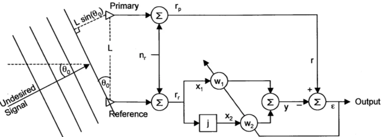
\ 'Output

ference _X2

J W2

Figure 2-7: Two-antenna receive beamforming that uses LMS interference cancella-tion with system input x, receiver noise n, filter output y, plant output r, and error

E [11, p. 373].

to the primary receiver in the direction of propagation. It can be expressed as

0 27rLosin(60) (2.34)

Aowo

where AO is the wavelength, LO is the distance between the primary and reference receivers, and 0 is the angle of propagation relative to the receivers shown in Figure

2-7.

Adaptive beamforming uses the LMS algorithm with complex weights. Real weights would allow the gain of the received signal to be modulated. However, the benefit of using complex weights is that both the gain and phase of the received sig-nal can be adjusted. Adjusting the phase of a received sigsig-nal is vital to beamforming because it allows the two received signals to augment or cancel each other through constructive or destructive interference. Complex weights can be represented by two real weights: one representing the real (in-phase) part, and the other representing the imaginary (quadrature) part. The imaginary weight is simply shifted by 90 degrees, which is equivalent to multiplying it by

j

With complex weights configured as a pair of real weights, shown in Figure 2-7, the LMS algorithm can be used to place a null in a certain direction. The LMS

beam-forming algorithm is set up such that the error is the difference between the primary and reference receivers. Therefore, minimizing the error will cause the weights to configure themselves such that the reference and primary signals cancel each other in the chosen direction.

The optimal weights can be found in a way similar to the method from Section

2.3. This method follows the proof from [11, p. 372]. The weight vector is a complex

number that represents the phase shift necessary to form a null. Its parts w1 and

w2 form the real and imaginary components of this complex number. As Figure 2-7 shows, the vector x[n] sent to the weights is

x = r.n [n] 1 Arcos(won + wo6o) + nr[n] (2.35)

]

Arsin(won

+

wo

o)

+

nr[n]

The process to find the optimal weights follows by determining the autocorrelation matrix R[n]. This is found to be

R[n] = E[xxH]

&A

L

₂

_{0 r Ar(2.36)}

+

,2

01

where o is the noise variance of r. The result of (2.36) is possible due, to the properties of orthogonality from (2.26) and (2.27). Specifically, the cross-correlation of a cosine and sine of the same frequency is zero.

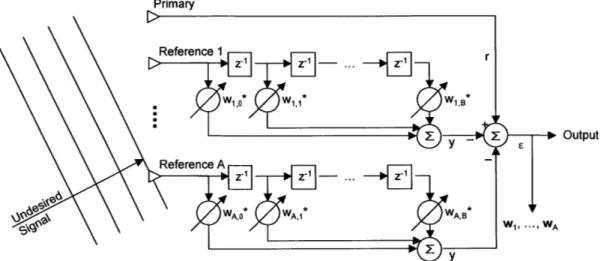
Primary

-+ Output

Reference A - Z1

005

wA,0* WA,1* WA,B

Figure 2-8: Traversal adaptive array for wideband beamforming.

between the input x and the primary receiver signal rp. This results in

p[n] = E[rpx]

E[Arcos(won)ArCOS(won +

wo6o)]

E[ArCOS(won)Arsin(won + wo6o)]

A2CO

1(.7

2

osir

(wooo)

J

Again, this result relies on sinusoidal orthogonality. Conveniently, the noise variance does not appear in p[n] because r, is uncorrelated with x. With R[n] and p[n] determined, the optimal weights w0rt can finally be calculated as

wopt[n] = R-1 [n]p[n]

A 2 cos(WOoo) A2

_{A +2r sin(o60}

+2U2

[](2.38)

using the Weiner solution (2.17). These optimal weights will allow the two-antenna narrowband system to form a null in the direction of 00.

Additional receivers allow for greater degrees of freedom in placing multiple nulls. In addition, it is possible to place the high gain region in the direction of a SOI in order to maximize its SNR. Wideband signals, however, contain multiple frequencies, and single complex weights and phase shifting may not be sufficient in an adaptive array. For wideband signals, a traversal adaptive array is required [11, p. 399]. As shown in Figure 2-8, the traversal adaptive array not only has the benefit of spatial beamforming, but also has the signal cancellation architecture necessary to process wideband signals.

2.9

Transmit Adaptive Beamforming

Transmit adaptive beamforming is another method of adaptive directional cancella-tion. In this case, each transmitter in an array adjusts its gain and phase such that a null is placed in the direction of the designated receiver. Although a relatively new topic in field of communications, such a strategy can be useful for any wireless application that can be improved by full duplex communication [6].

In this application of transmit beamforming, it is desired that the power at the re-ceiver be zero. Adaptive filtering is naturally useful for such an optimization problem. In a conventional LMS filter, the gradient of the performance surface is derived from reducing the error to zero. Here, the performance surface is the power at the receiver, and a gradient function can be found in terms of the weights in each transmitter's adaptive filter.

To find a function for the power, we must first derive the transmitted signal. Each transmitter contains an adaptive filter with weights w that act on the reference input

x[n]. The reference input is common to all of the transmitters but each transmitter's

weights can take different values. In any system with a transmit filter, the transmitted signal from transmitter a is

ta[n] = x[n] * Wa (2.39)

where "*" stands for convolution. The transmitted signal travels through the air to reach the receiver. On the way, it may reflect off of different surfaces, causing delays in the signal arrival times. The basic natural phenomena that impact signal propagation are reflection, diffraction, and scattering [16]. The entire collection of gains and delays due to these mechanisms is known as the "channel", and can be represented as a transfer function vector h from the transmitter to the receiver. In a

system with A transmitters, the signal at the receiver r[n] is

A

rfn] = E x[n]I*w* ha. (2.40) a=1

By definition, the power at the receiver is the square magnitude of the received signal.

The power p[n] is

p[n]

r[n]|2.

(2.41)

It is often convenient to express the signal r[n] as a vector r. This allows normally complicated operations to be expressed as matrix multiplication. The result from

(2.40) can be expressed as

r = Ew (2.42)

where w is a vector that contains all of the weight values for every transmitter and

E is a matrix that is derived from w and h. A full derivation of E is given in Section

4.1. With this notation, the power at the receiver is

p = WTETEw. (2.43)

Another important condition required for transmit beamforming is that the total transmitted power remains constant. This condition is important because otherwise, the easiest way to achieve zero power would be to set the weight values to zero. This condition can be expressed as

wTw =1. (2.44)

found via the method of Lagrangian multipliers [7, p. 1981. If we label the functions

f

g

h = 1, (2.45)

then we may specify the Lagrange function A as

A =

f+A(g-h)

= WTETEw

+

where A is the Lagrangian multiplier. The Lagrange function takes a form of the Rayleigh quotient [13, p. 440] and it is already apparent that the optimal w will be an eigenvector of ETE. However, we will carry out the rest of the proof by taking the gradient of the Lagrange function and setting it to zero in order to determine its critical points. When we carry out the operation VA = 0, we find that

aA

aA

+

The result from (2.48) simply restates the constraint from (2.44). However, the result from (2.48) proves that the optimal w is an eigenvector of ETE. In addition, the corresponding A is an eigenvalue of ETE.

of (2.43) given the constraint (2.44). However, the optimal weight vector must still be chosen from this set of critical points. The power can be determined from (2.48) as

ETEw = Aw

wTETEw = wTAw = wTwA

p

=

In other words, the value of the power at a critical point of (2.43) is an eigenvalue of ETE. Since we want to minimize the power on the receiver, the optimal weight vector will be the eigenvector that corresponds to the smallest eigenvalue.

Chapter 3

Methods and Algorithms for

Multiple-Input Single-Output

(MISO) Active Cancellation

The basic STAR system uses a single receiver and multiple transmitters. The reason

for this is that multiple transmitters allow for beamforming methods to create a null

at the receiver. This is desirable because the analog receiver chain and the

analog-to-digital converter are intended for low power signals. High signal power will saturate

and possibly destroy the receiver's electronics [2, p.

8].

Multiple receive antennae arranged in a phased array can function to create a

far-field receive-side null in the direction of the transmitter. However, any signal of

interest coming from the direction of the undesired transmitter will not be picked up

by the receiver if such a directional null is used. Since the transmitters are stationary

with respect to the receiver, these signals of interest will not be detected until the

entire platform changes orientation. One exception would be if instead of a directional

null, a near-field receive-side null is formed at the transmitter. However, forming a

receive-side null at the transmitter is not useful to the STAR system unless the receiver

saturation problem is first solved.

In contrast to receive beamforming, transmit beamforming allows a single receiver

to function as an isotropic antenna and detect signals of interest from every angle.

This is possible because the transmissions can be adjusted to create a null in the

interference pattern at the receiver. In fact, there are usually many different far-field

interference patterns that result in a null at the receiver [17, p. 81].

One way to form a null at the receiver is to adjust the gain and phase of the

transmitters. Under ideal conditions, this would be the best solution for narrow band

transmitter signals [4, p. 8]. However, signals with multiple frequencies react

differ-ently to fixed delays, and so beamforming becomes difficult with only two adjustable

values per transmit antenna [4, p. 12]. In addition, the channel between the

trans-mitters and the receiver is likely to include reflections. Reflections translate to delays

and gains in the channel's impulse response [11, p. 201]. For these reasons, the initial

multiple-transmitter, single-receiver system uses an adaptive filter on each

transmit-ter. These adaptive filters allow the issues of reflections and wide band signals to be

addressed by increasing the number of filter taps. The lower limit to successful

trans-mit beamforming is two transtrans-mitters. With knowledge of the channels, two adaptive

antennae can theoretically be configured such they cancel at the receiver. This lower

limit may not be valid if the channel length is much greater than the number of taps.

This chapter will present three methods of transmit beamforming and two methods

of obtaining a channel estimate. These methods all assume multiple transmitters and

a channel that can be modeled by its impulse response. In each case, the channel

is allowed to vary with time. Practical signal processing applications must account

for a time-variant channel even if the antenna platform is stationary [4, p. 62]. It is

important to note that none of the methods presented in this chapter require inverting

a matrix or finding its eigenvalues. This is very beneficial because large inverse or

eigenvalue operations require excessive computation time and resources.

3.1

Transmit Beamforming Method: Trial and

Er-ror

The most basic method of using adaptive filters in transmit beamforming involves adjusting the filter weights through trial and error. Appendix A.1 gives the Matlab code for this operation. As shown in Figure 3-1, the only adaptive filters in the entire system are located on the transmitters. In this system, there are A transmitters and each transmitter has B weights. Operation of the system requires an arbitrary time period K for which samples can be collected every time a weight is adjusted. The size of K will be mentioned in Section 3.2. Figures 3-2 and 3-3 show that every K cycles, a particular weight from one of the filters is increased by a small step amount. The new average power pag is then obtained by taking a moving average over the past K measurements of the power seen at the receiver. The received signal r[m] represents a voltage or current. Therefore, the average power is related to the square of the received signal, as shown by [10, p. 116]

pavg[n] =

K

m=n-K

where n represents the sample number or time. If the new average power is less than the old average power, the weight is left at its new value. Otherwise, it is decreased

by twice the step width. At each weight step, all the weights are re-normalized to

a specified constant weight power Wowe, so as to keep the transmit power constant. The normalization is accomplished by setting the new weight vector w[n + 1] [7, p.

100]

w[n + 1] = w[n] WTow[) 2 (3.2)

(wT[n] -w[n]f)i

This procedure causes all of the weights to change every cycle. However, the overall change in power still largely reflects the change in the stepped weight.

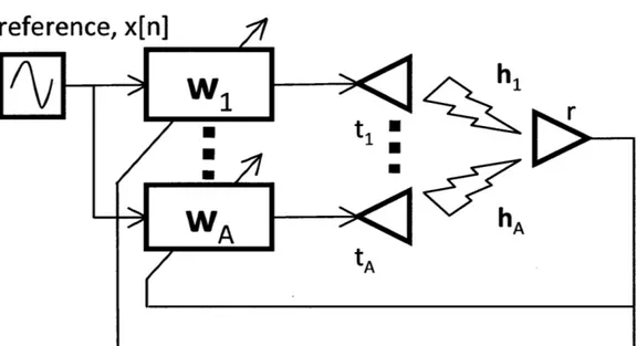
reference, x[n]

Figure 3-1: System block diagram for a STAR approach using adaptive filters on the transmitters. The transmit weight vector for transmitter a is Wa and the channel

between transmitter a and the receiver is ha.

K cycles K cycles Step weight 1 Test weight 1,

Step weight 2

Test weight 2,

Step weight 3 MEN , Test weight A-B,Step weight 1

Figure 3-2: Trial and Error algorithm timing diagram. There are A transmitters and

B weights per transmitter, therefore, there are A x B weights total.

Figure 3-3: Trial and Error algorithm decision flow chart. This shows the algorithm's computation and decision processes every K cycles.

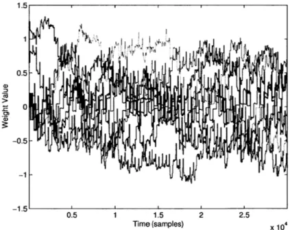
Even with very fine tuning, the performance of this method leaves much to be desired. The weights take a very long time to properly converge, and significant power spikes are produced even at convergence. As Figure 3-4 shows, this method obtains only minimal cancellation. Figure 3-5 reveals that the power spikes are caused

by the sharp steps in weight value. It also shows that the weights never really settle.

Despite all of its disadvantages, one benefit of this method is that it is virtually immune to noise since all of the calculations use averages of the received data.

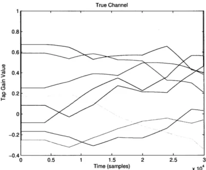
The convergence of the weights is largely affected by the speed at which the channel varies. Figure 3-6 shows one realization of the random time-variant channel model that will be used in all the simulations of this chapter. In every method presented, the weights converge more finely if the channel changes slowly.

0 0.5 1 1.5 2 2.5 3

Time (samples) _{x 10}4

Figure 3-4: Received power relative to transmitted power for the Trial and Error method. In this simulation, A = 2, B = 4, K = 100, and the weights were stepped by 0.1 every K cycles. The channel model varies with time, as shown in Figure 3-6.

0.5 1 1.5 2 2.5

Time (samples) _{x 10}4

True Channel 04 -L 0.2 0--0.2 -0.4 0 0.5 1 1.5 2 2.5 3 Time (samples) _{x 10,}

Figure 3-6: Channel realization from the simulation in Figure 3-4. The channel from each transmitter to the receiver has four taps. Each line indicates how the tap values change with time. Every 4000 samples, the slope of these lines changes to a random number between -g and .

Figure 3-7: System block diagram for a STAR approach that requires a channel estimate for transmit beamforming.

3.2

System Identification for Channel Estimation

In contrast to the previous method of transmit beamforming in Section 3.1, all other methods require a channel estimate. The channel estimate is useful because it allows for more sophisticated and intelligent algorithms to be used in the transmitter adap-tive filters. For these algorithms, a channel must be estimated from each transmitter to each receiver. A good way to estimate the channel is to use a system identification adaptive filter [18, p. 162]. The system block diagram of Figure 3-7 represents the basic layout used in any method that requires a channel estimate. The issue of actu-ally estimating the channel will be addressed in Section 3.5. For now, the descriptions of these transmit beamforming methods will assume that the channel estimates are perfectly accurate.

An estimate of the average signal power at the receiver is required in order to reduce the actual signal power impinging on the receiver. This estimate can be

calculated in terms of known variables and signals. In order to derive the average power estimate, it is important to show how this estimate relates to the actual received signal. The signal r[n] at the receiver is the sum over all A transmitters of each transmitter signal ta [n] convolved with its respective channel ha between transmitter and receiver. The transmitter signal itself is a convolution between the transmitter weights w, and some common reference signal

xfn].

The receiver ultimately sees the sum of each double convolution of the reference, transmitter weights, and channel for each transmitter as shown by

A r [n] E tan] a=1 A = x[n] * wa * ha. (3.3) a=1

Every cycle, a prediction of the received signal is calculated by

A

rpred[r] n x3n] * Wa * heet,a . (3.4)

a=1

This prediction rpred[n] is based on the current values of the reference signal, trans-mitter weights, and channel estimate he,t,a. The channel estimate comes from copying the weights of the receiver's system identification LMS filters. Once a prediction is obtained for the received signal, it is used to determine a prediction for the average power as

Pavg,pred[fl

=

K

rpred [m]

(3.5)

m=n-K

K of elements that were taken from the reference signal. It is necessary for K to be

large enough such that (3.5) can average over enough samples to include the delays

due to w and h. The smallest value for K is the length of the impulse response of

w

*

h, which is equal to the sum of the lengths of w and h.

3.3

Transmit Beamforming Method: Gradient

De-scent

The transmit beamforming method discussed in this section directly optimizes the received power using a gradient calculation. This method requires a channel estimate. The derivation for the formula used to calculate the weight update vector is similar to that of the LMS algorithm. As explained in Section 2.4, the LMS algorithm uses the instantaneous squared error E2 [n] as an estimate of the mean squared error E[e2 [n]]. The negative gradient vector of the power, -V[n], points in the direction that most directly minimizes the mean squared error and contains the weight direction and magnitude with which to update each weight [11, p. 21]. Once the gradient is calculated, the weights themselves are updated in the same way as the LMS filter, given in (2.20) where p is the adjustable growth factor.

As previously shown in (2.19), V[n] is calculated by taking the partial derivative with respect to each weight. Similar to the LMS algorithm, the gradient vector for the transmit beamforming method of this section is also calculated using partial derivatives. The main difference is that the LMS algorithm attempts to minimize the mean squared error of the filter [11, p. 100], whereas here we attempt to minimize the average signal power at the receiver. In this sense, the performance surface of the algorithm discussed in this section is the average receiver power as a function of each weight in each transmitter's adaptive filter.

The negative gradient vector is the vector of steepest descent along the perfor-mance surface. The average power gradient vector for transmitter a is

0 Pavg,pred [n) &Pavg,pred[fl] 09Wa, 1 Va[n] - (3.6)

aa

-As shown in (3.5), the predicted average power Pavg,pred[n] is a function of the predicted received signal rpred[n]. In addition, (3.4) shows that rpred[n] is a function of x[n], wa,

and heet,.. Since x[n] and hest,a are constant during this partial derivative calculation,

rpred[n] is really just a linear function of each Wab. Using the chain rule,

Va[n] = 9Pavgpred[f] OWa S(pag,pred[n] _orPed[] (3.7) arpred[n] OWa _(3.

2

K

~Z

Note that the partial derivative in (3.7) only evaluates to the solution in (3.8) when the samples in rpred are real. The original predicted power in (3.5) uses

|rpredl,

The received signal prediction rpred[n] is the sum of the signal contributions from each transmitter. A prediction for the contribution from transmitter a can be ex-pressed as rpred,a[n] = (x[n] * hest,a) * Wa = ga[r] * Wa B - g[n - b]wa,b. (3.9) b=1

Since each weight Wa,b in a traversal filter with weight vector Wa represents a gain and a delay [10, p. 5], this equation depicts how the weight vector is convolved with the other terms. It is now apparent that the partial derivative of the received signal with respect to each weight is

arpred [n] = ga[n - b] . _(3.10)

From this equation and (3.9), it is finally possible to determine the gradient vector from (3.8) to be rpredIm)gaIm - 11 Va[n] = .Z(3.11) m=n-K rpred[m]ga[m -

B]

Appendix A.2 gives the Matlab code for the entire operation.

The method of this section performs much better than the method of Section

3.1. As shown by the simulation results of Figure 3.3, the average received power can

drop to 20dB below the transmit power within 30000 samples. Another benefit of this method is that it uses direct calculation. This method does not use any conditional statements such as those shown in Figure 3-3 to test or compare, making it linear in terms of the weights and much more mathematically sound overall.

However, this method is not without its flaws. The first potential problem is the speed of convergence. The system has a good steady state average power and has good long term behavior in general. However, if one of the channels were to undergo a large change in a small amount of time, the long transient response could pose problems for achieving the goals of STAR. Another potential problem with this system is that the power at the receiver does not remain constant after the weights have converged. The simulation from Figures 3.3 and 3-9 shows that even after convergence, the received power ranges from -15dB to -25dB relative to the transmitter. Such behavior is no surprise considering that the transmitter weights are also somewhat mobile after convergence.

It should be noted that the performance of this method is heavily dependent on the growth factor. When the growth factor was lowered from 0.02 to 0.005, it caused the weights to be much more stable and lowered the average receive power by an additional 5dB as displayed in Figure 3-10. However, with a smaller growth factor,

0 0.5 1 1.5 2 2.5 3

Time (samples) x 104

Figure 3-8:

method. In

with time.

Received power relative to transmitted power for the Gradient Descent

this simulation, A = 2, B = 4, and p-L

= 0.05. The channel model varies

0.5 1 1.5 2 2.5

Time (samples) X 104

Figure 3-9: The adaptive filter weights from the simulation in Figure 3.3.