Dynamic Effects of Credit Shocks in a Data-Rich Environment

Texte intégral

(1)2013s-11. Dynamic Effects of Credit Shocks in a Data-Rich Environment Jean Boivin, Marc P. Giannoni, Dalibor Stevanović. Série Scientifique Scientific Series. Montréal Mai 2013. © 2013 Jean Boivin, Marc P. Giannoni, Dalibor Stevanović. Tous droits réservés. All rights reserved. Reproduction partielle permise avec citation du document source, incluant la notice ©. Short sections may be quoted without explicit permission, if full credit, including © notice, is given to the source..

(2) CIRANO Le CIRANO est un organisme sans but lucratif constitué en vertu de la Loi des compagnies du Québec. Le financement de son infrastructure et de ses activités de recherche provient des cotisations de ses organisations-membres, d’une subvention d’infrastructure du Ministère du Développement économique et régional et de la Recherche, de même que des subventions et mandats obtenus par ses équipes de recherche. CIRANO is a private non-profit organization incorporated under the Québec Companies Act. Its infrastructure and research activities are funded through fees paid by member organizations, an infrastructure grant from the Ministère du Développement économique et régional et de la Recherche, and grants and research mandates obtained by its research teams. Les partenaires du CIRANO Partenaire majeur Ministère de l'Enseignement supérieur, de la Recherche, de la Science et de la Technologie Partenaires corporatifs Autorité des marchés financiers Banque de développement du Canada Banque du Canada Banque Laurentienne du Canada Banque Nationale du Canada Banque Scotia Bell Canada BMO Groupe financier Caisse de dépôt et placement du Québec Fédération des caisses Desjardins du Québec Financière Sun Life, Québec Gaz Métro Hydro-Québec Industrie Canada Investissements PSP Ministère des Finances et de l’Économie Power Corporation du Canada Rio Tinto Alcan State Street Global Advisors Transat A.T. Ville de Montréal Partenaires universitaires École Polytechnique de Montréal École de technologie supérieure (ÉTS) HEC Montréal Institut national de la recherche scientifique (INRS) McGill University Université Concordia Université de Montréal Université de Sherbrooke Université du Québec Université du Québec à Montréal Université Laval Le CIRANO collabore avec de nombreux centres et chaires de recherche universitaires dont on peut consulter la liste sur son site web. Les cahiers de la série scientifique (CS) visent à rendre accessibles des résultats de recherche effectuée au CIRANO afin de susciter échanges et commentaires. Ces cahiers sont écrits dans le style des publications scientifiques. Les idées et les opinions émises sont sous l’unique responsabilité des auteurs et ne représentent pas nécessairement les positions du CIRANO ou de ses partenaires. This paper presents research carried out at CIRANO and aims at encouraging discussion and comment. The observations and viewpoints expressed are the sole responsibility of the authors. They do not necessarily represent positions of CIRANO or its partners.. ISSN 1198-8177. Partenaire financier.

(3) Dynamic Effects of Credit Shocks in a Data-Rich Environment* Jean Boivin †, Marc P. Giannoni ‡, Dalibor Stevanović§. Résumé / Abstract We examine the dynamic effects of credit shocks using a large data set of U.S. economic and financial indicators in a structural factor model. The identified credit shocks, interpreted as unexpected deteriorations of credit market conditions, immediately increase credit spreads, decrease rates on Treasury securities, and cause large and persistent downturns in the activity of many economic sectors. Such shocks are found to have important effects on real activity measures, aggregate prices, leading indicators, and credit spreads. Our identification procedure does not require any timing restrictions between the financial and macroeconomic factors, and yields interpretable estimated factors. Mots clés/keywords : Credit shock, structural factor analysis. Codes JEL : E32, E44, C32. *. The views expressed in this paper are those of the authors and do not necessarily reect the position of Finance Canada, the Federal Reserve Bank of New York, or the Federal Reserve System. † Finance Canada; e-mail: jean.boivin@fin.gc.ca ‡ FRB of New York, 33 Liberty Street, New York, NY 10045; e-mail: marc.giannoni@ny.frb.org § Université du Québec à Montréal, Département des sciences économiques, 315, rue Ste-Catherine Est, Montréal, QC, H2X 3X2; e-mail: dstevanovic.econ@gmail.com.

(4) 1. Introduction. The recent financial crisis caused the most important global economic downturn since the Great Depression. It renewed interest in properly understanding the connection between the real economy and the financial sector. This is important for various reasons. First, by their forward-looking nature, asset prices and credit spreads (the difference between corporate bond yields and yields on same-maturity Treasury securities) should be useful in predicting fluctuations of economic activity, at least in theory (see, e.g., Philippon, 2008). Studies, among others, by Stock and Watson (1989, 2003), Gertler and Lown (1999), and more recently by Mueller (2007), have found that credit spreads do have significant forecasting power in predicting economic growth. In addition, while corporate bond yields incorporate information about future economic conditions, Gilchrist, Yankov and Zakrajˇsek (2009), henceforth GYZ, show that shocks to corporate bond yields — based on a broad set of individual firms’s bond prices instead of relying on common aggregate credit spread indices — cause significant fluctuations in economic activity. Indeed, the strong tightening in US credit conditions in 2007 and 2008 and the associated contraction in economic activity that followed suggests that credit conditions may have important effects on the economy. Understanding the joint dynamics of the real economy and the financial sector could lead to more timely – and hopefully more pre-emptive – policy responses. This calls for a comprehensive analysis of the quantitative effects of credit shocks on US economic variables and requires an empirical framework that is sufficiently rich to capture the information necessary to account for these joint dynamics. In this paper, we re-examine the evidence concerning the propagation mechanism of credit shocks on economic activity and other key macroeconomic variables. We characterize the dynamic effects of credit shocks using a structural factor model, or Factor-Augmented VAR (FAVAR) estimated with large panels of U.S. monthly and quarterly data. In contrast to standard structural VAR models, factor models have a number of advantages: i) they 1.

(5) permit considering the large amount of information potentially observed by agents, and so minimize the risk of omitted variable bias; ii) they are not sensitive to the choice of a specific data series, which may be arbitrary, to represent a general economic concept; iii) they are less likely to be subject to non-fundamentalness issues raised by Forni et al. (2009); and iv) they allow us to compute the response of a large set of variables of interest to identified shocks. The empirical model is estimated using a large number of US time series. We proceed in two steps. First, in order to recover the space spanned by structural shocks (including shocks to credit spreads), we estimate factors as principal components from standardized data panels. These common factors are supposed to capture the key aggregate fluctuations in economic and financial series. All economic and financial indicators may be decomposed into a component contemporaneously related to the common factors, and a series-specific (idiosyncratic) component which is unrelated to aggregate conditions. Then, a finite-order VAR approximation of the factors dynamics is estimated. The identification of shocks to credit conditions is achieved by imposing restrictions on the impact matrix of the structural shocks on a few selected observable variables, as proposed by Stock and Watson (2005). This allows us to impose the minimum amount of restrictions necessary to identify shocks to credit conditions. The empirical approach is related to that of GYZ, but differs from it in important ways. In order to determine their credit shocks, GYZ impose potentially strong identifying assumptions. In particular, they assume that no macroeconomic variable, including measures of economic activity, prices or interest rates can respond contemporaneously to credit shocks. This assumption may be restrictive, e.g., if changes in credit spreads affect contemporaneously overall financial conditions, including interest rates. It may potentially attribute an overly strong effect of credit spreads on economic variables by preventing a possible contemporaneous drop in the yield on riskless securities, which might mitigate the effect of a credit. 2.

(6) tightening. In addition, GYZ assume that the factors summarizing macroeconomic indicators are contemporaneously uncorrelated with the factors summarizing all credit spreads, regardless of the source of disturbances. To the extent that such assumptions are violated, their results might be contaminated. In our identification schemes, these assumptions are relaxed. Our results show that an unexpected increase in credit spreads causes a significant contemporaneous drop in yields of Treasury securities at various maturities, and has a significant effect in the same month on other variables such as consumer expectations, commodity prices, capacity utilization, hours worked, housing starts, etc, in contrast to GYZ’s assumption. This unexpected increase in the external finance premium also results in a significant and persistent economic slowdown, in the months following the shock. The responses generated by our identifying procedure yield a realistic picture of the effect of credit shocks on the economy, and provide valuable information about the transmission mechanism of these shocks. In addition, we find that the extracted common factors capture an important dimension of the business cycle movements. Furthermore, we find that credit shocks have quantitatively important effects on several indicators of real activity and prices, leading indicators, and credit spreads, as they explain a substantial fraction of the variability of these series. Results from a counterfactual experiment indicate that the credit shocks explain a large part of the decline in many activity and price series, as well as the Federal Funds Rate in 2008 and 2009. This is in line with recent findings of Stock and Watson (2012). Finally, a further advantage of the identification procedure is that it allows us to recover underlying “structural” factors that have an interesting economic interpretation. Those factors can be obtained by judiciously combining the initially extracted factors. Our empirical analysis considers a battery of specifications. These findings are robust to different data frequencies and identification schemes. The first FAVAR model that we consider is estimated using a monthly balanced panel. We impose a recursive assumption. 3.

(7) to identify structural shocks. The responses of key macroeconomic series to credit shocks are found to be qualitatively similar to those from a small-scale VAR model. However, credit shocks are found to generate a substantially larger share of economic fluctuations in the FAVAR model than in the small-scale VAR. Given that the VAR likely omits relevant information, this suggests that the VAR may be misspecified and does not properly capture the source or propagation of key structural shocks. In addition, the factor model gives a more complete and comprehensive picture of the effects of credit shocks since the impulse responses and the variance decomposition of all variables can be obtained. As mentioned above, our approach produces interpretable common factors. Indeed, the first structural factor is highly correlated with price measures, the second factor is important for the unemployment rate, while the third is related to interest rates, and the fourth factor is correlated with credit spreads. In the second specification, we consider a mixed-frequencies monthly panel, using also quarterly data. We impose a recursive identification scheme where we explicitly distinguish between the monetary policy shocks and credit shocks, although the Federal funds rate (the instrument of policy) is allowed to respond on impact to credit shocks. The results are similar to those from the previous model, except that interest rates fall significantly on impact in response to credit shocks. Again, we obtain interpretable factors. As a part of robustness analysis, we consider a quarterly balanced panel and identify the structural shocks using sign restrictions, as well as two FAVAR specifications with observable factors. Overall, the results are quite robust: in each specification, an adverse shock to credit conditions causes a significant and persistent economic downturn. This reinforce our empirical evidence about the real effects of financial disturbances on economic activity. In the next section, we briefly review some mechanisms linking credit shocks and economic variables. Section 3 presents the structural factor model and discusses various estimation and identification issues. The main results are presented in Section 4, followed by the robustness. 4.

(8) analysis. In Section 6, we compare the results to those obtained from smaller-scale structural VAR models. Section 7 concludes. The Appendix presents the impulse response results after a monetary policy shock and a description of the data sets.. 2. Some Theory. In this section we briefly review various mechanisms that connect financial and economic variables, and the channels through which shocks on the credit market could affect economic activity. Financial frictions are crucial when linking the credit market conditions to economic activity. In their presence, the composition of the borrowers’ net worth becomes important due to the incentive problems faced by the lenders [Bernanke and Gertler (1995), and Bernanke, Gertler and Gilchrist (1999)]: a borrower with a low net worth relative to the amount borrowed has a higher incentive to default. Given this agency problem, the lender demands a higher premium to provide external funds, which raises the external finance premium. Therefore, economic downturns and associated declines in asset values tend to produce an increase in the external finance premium for borrowers holding these assets in their portfolio. The higher external finance premium, in turn, leads to cuts in investments, and hence in production, employment, and thus in the overall economic activity, which induces asset prices to fall further, and so on. This is essentially the so-called financial accelerator mechanism. Several other transmission channels, focusing on the credit supply, have also been introduced in the literature. The narrow credit channel focuses on the health of the financial intermediaries and their agency problems in raising funds. The capital channel can transmit credit conditions to the economic activity, if banks’ capital is affected. In that case, banks must reduce the supply of loans, resulting in a higher external finance premium. In summary, Bernanke and Gertler (1995) identify two channels through which a shock to the external finance premium can affect the real activity: 5.

(9) 1. Balance sheet channel, according to which a deterioration of a firm’s net worth results in an increase of its external finance premium, and thus causes a reduction in investment, employment, production, and prices. This can be broadly seen as affecting the demand of credit. 2. Bank lending channel, according to which a deterioration of the financial intermediaries’ external finance premium constrains the supply of loans and hence causes a reduction in economic activity. More recently, credit risks and their effect on economic conditions have been modeled in a general equilibrium framework. For instance, Christiano, Motto and Rostagno (2003, 2009, 2013), in a series of papers, augment a medium-size DSGE model similar to Christiano, Eichenbaum and Evans (2005) and Smets and Wouters (2007) with a financial accelerator mechanism linking conditions on the credit market to the real economy through the external finance premium following Bernanke, Gertler and Gilchrist (1999). They furthermore introduce a so-called “risk shock,” which captures the exogenously time-varying cross-sectional standard deviation of idiosyncratic productivity shocks, and which directly moves credit spreads by changing agency costs. Christiano, Motto and Rostagno (2003), find that such “risk shocks” account for a large share of US GDP fluctuations. In addition, Gilchrist, Ortiz and Zakrajˇsek (2009) estimate a similar model in which they introduce two financial shocks: a financial disturbance shock that directly affects the external finance premium (corresponding to the “risk shock” just discussed), and a net worth shock affecting the balance sheet of a firm. The second shock can be viewed as a credit demand shock, whose effect depends on the degree of financial market frictions. After estimating the structural model using US data covering the 1973-2008 period, Gilchrist, Ortiz and Zakrajˇsek (2009) find that both financial shocks cause an increase in the external finance premium, which, through the financial accelerator, implies a persistent slowdown in economic activity and in investment.. 6.

(10) 3. Econometric Framework in Data-Rich Environment. It is common to estimate the effects of identified macroeconomic shocks using small-scale vector autoregressions (VARs). However, small-scale VAR models present several issues. Due to the small amount of information in the model, relative to the information set potentially observed by agents, the VAR can easily suffer from an omitted variable problem that can affect the estimated impulse responses or the variance decomposition. Related to that, Forni et al. (2009) argue that while non-fundamentalness is generic of small scale models, it is highly unlikely to arise in large dimensional dynamic factor models1 . In addition, a potential problem pertains to the choice of a specific data series to represent a general economic concept, which may be arbitrary. Finally, even if the previous problems do not occur, we can produce impulse responses only for the variables included in the VAR. One way to address all these issues is to take advantage of information contained in large panel data sets using dynamic factor analysis, and in particular the factor-augmented VAR (FAVAR) model. The importance of large data sets and factor analysis is now well documented in both forecasting and structural analysis literature [see Bai and Ng (2008) for the overview]. In particular, Bernanke, Boivin and Eliasz (2005) and Boivin, Giannoni and Stevanović (2009), have shown that incorporating information through a small number of factors corrects for various empirical puzzles when estimating the effects of monetary policy shocks. We consider the static factor model2. Xt = ΛFt + ut ,. (1). Ft = Φ(L)Ft−1 + et ,. (2). 1. If the shocks in the VAR model are fundamental, then the dynamic effects implied by the moving average representation can have a meaningful interpretation, i.e., the structural shocks can be recovered from current and past values of observable series. 2 It is worth noting that the static factor model considered here is not very restrictive since an underlying dynamic factor model can be written in static form [see Stock and Watson(2005)].. 7.

(11) where Xt contains N economic and financial indicators, Ft represents K unobserved factors (N >> K), Λ is a N × K matrix of factor loadings, ut are idiosyncratic components of Xt that are uncorrelated at all leads and lags with Ft and with the factor innovations et . This model is an approximate factor model, as we allow for some limited cross-section correlation among the idiosyncratic components in (1).3. 3.1. Estimation. The unknown coefficients in (1)–(2) could in principle be estimated by Gaussian maximum likelihood using the Kalman filter (or by Quasi ML), as shown in Engle and Watson (1981), Stock and Watson (1989), and Sargent (1989). This method is however computationally burdensome and is likely to lead to misspecification when N is very large.4 We adopt instead an alternative estimation approach based on a two-step principal components procedure, where factors are approximated in the first step, and the dynamic process of factors is estimated in the second step. We rely on the result that factors can be obtained by a Principal Components Analysis (PCA) estimator. Stock and Watson (2002a) prove the consistency of such an estimator in the approximate factor model when both cross-section and time sizes, N , and T , go to infinity, and without restrictions on N/T . Moreover, they justify using Fˆt as regressor without adjustment. Bai and Ng (2006) furthermore show that √ √ PCA estimators are T consistent and asymptotically normal if T /N → 0. Inference should take into account the effect of generated regressors, except when T /N goes to zero. The principal components approach is easy to implement and does not require very 3. We assume that only a small number of largest eigenvalues of the covariance matrix of common components may diverge when the number of series tends to infinity, while the remaining eigenvalues as well as the eigenvalues of the covariance matrix of specific components are bounded. See Bai and Ng (2008) for an overview of the modern factor analysis literature, and the distinction between exact and approximate factor models. 4 Recently, significant improvements have nonetheless been proposed to this approach. For instance the Kalman filter speedup by Jungbacker and Koopman (2008), using principal components for starting values and then a single pass of the Kalman filter by Giannone, Reichlin, and Sala (2004), and principal components for starting values then use EM algorithm to convergence by Doz, Giannone, and Reichlin (2006).. 8.

(12) strong distributional assumptions. Simulation exercises have shown that likelihood-based and two-step procedures perform quite similarly in approximating the space spanned by latent factors5 . However, since the unobserved factors are first estimated and then included as regressors in the VAR equation (2), and given that the number of series in our application is small, relative to the number of time periods, the two-step approach suffers from a “generated regressors” problem. To get an accurate statistical inference on the impulse response functions that accounts for uncertainty associated to factors estimation, we use the bootstrap procedure as in Bernanke, Boivin and Eliasz (2005).. 3.2. Identification of structural shocks. A key objective of this paper is to identify the effect of shocks to credit conditions on the economy be imposing a minimal number of restrictions. To identify the structural shocks, we employ the contemporaneous timing restrictions procedure proposed in Stock and Watson (2005). This procedure identifies credit shocks by restricting only the responses on impact of a few economic indicators. This approach has the advantage of leaving the dynamics of the factors unconstrained, and allows the identified structural shocks to have contemporaneous effects on all factors driving our panel of indicators. The approach adopted here contrasts with GYZ, who assume that credit shocks do not have a contemporaneous effect on any of the economic factors and indicators, including interest rates. Furthermore, unlike GYZ who estimate two orthogonal sets of factors — those explaining a panel of economic activity indicators, and factors related to credit spreads 6 — we do not need to make such a distinction, and thus do not need to assume that financial factors are orthogonal to other economic factors. Finally, contrary to other identification strategies 5. See, Doz, Giannone and Reichlin (2006). Moreover, Bernanke, Boivin and Eliasz (2005) estimated their model using both two-step principal components and single-step Bayesian likelihood methods, and obtained essentially the same results. 6 In GYZ, the credit shock is identified as an innovation to the first “financial factor”obtained as a principle component to a large panel of credit spread data.. 9.

(13) that have been adopted in analyses using FAVAR models, we do not need to impose that any factor be observed factor, nor do we rely on the interpretation of a particular latent factor to characterize the responses of economic indicators to structural shocks.7 To identify our credit shocks, we start by inverting the VAR process of factors (2), assuming stationarity, and substitute the resulting expression into (1), to obtain the movingaverage representation of Xt : Xt = B(L)et + ut ,. (3). where B (L) ≡ Λ[I − Φ(L)L]−1 . We assume that the number of static factors, K, is equal to the number of structural shocks and that the factor innovations et are linear combinations of structural shocks εt : εt = Het ,. (4). where H is a nonsingular square matrix and E[εt ε0t ] = I. Using (4) to replace et in (3) gives the structural moving-average representation of Xt : Xt = B ? (L)εt + ut ,. (5). where B ? (L) ≡ B(L)H −1 = Λ[I − Φ(L)L]−1 H −1 . To identify the structural shocks εt , we arrange the data in Xt and impose contemporaneous timing restrictions on the impact matrix in (5). Specifically, we assume that certain structural shocks do not affect the first few 7. In Bernanke, Boivin and Eliasz (2005) and Boivin, Giannoni and Stevanović (2009), the authors impose a short-term interest rate as an observed factor, and the monetary policy shock is identified as innovation in the interest rate VAR equation, after performing a Choleski decomposition.. 10.

(14) indicators in Xt within the period, so that the impact matrix takes the form         ? ? B0 ≡ B (0) =        .  x 0 ··· . x x .. . x x .. x .. .. x .. .. x x. 0   0     0  ,  ··· x   . . . ..  .    ··· x. where x stands for unrestricted elements. It is important to note that our identifying assumptions are imposed on the effects of structural shocks on particular indicators in our data set. They do not require latent factors not to respond contemporaneously to structural shocks. To estimate the matrix H, we proceed as in Stock and Watson (2005), noting that 0 ∗0 ∗ ? , where B0:K contains the first K rows of = B0:K Σe B0:K B0:K εt = B0:K et implies B0:K B0:K ? ? is = B0:K H −1 , and Σe is the covariance matrix of et . Since B0:K B0 ≡ B (0) = Λ, B0:K ∗ can be obtained by a K × K lower triangular matrix, then it must be the case that B0:K 0 ∗ 0 performing a Choleski decomposition of (B0:K Σe B0:K ), i.e.: B0:K = Chol(B0:K Σe B0:K ). It ∗ follows that H = (B0:K )−1 B0:K , or. 0 H = [Chol(B0:K Σe B0:K )]−1 B0:K .. (6). To estimate H, we just replace B0:K and Σe with their estimates in (6). The impulse responses to structural shocks in εt are obtained using (5). This identification procedure is similar to the standard recursive identification in VAR models, except that the series-specific term ut is absent in VARs. By imposing K(K − 1)/2 restrictions, we justidentify the K structural shocks.. 11.

(15) 3.3. Data and main specifications. In our application, we use two specifications of the FAVAR involving very different identifying restrictions and also an increasingly large number of economic and financial indicators. The time span for all panels starts in 1959M01 and ends in 2009M06. All series are initially transformed to induce stationarity. The description of the series and their transformation is presented in the Appendix. Common proxies of the external finance premium of borrowing firms are the credit spreads for non-financial institutions. Our benchmark measure will be the 10-year B-spread (i.e. the difference between BAA bond yields and Treasury bond yields), although we considered as alternatives the 10-year A-spread and the 1-year B-spread. Table 1 and Figure 7 summarize these measures. Figure 7 reveals clearly that credit spreads, especially the 1-year B-spread, are positively correlated with the unemployment rate. This correlation confounds however both the effects of current economic conditions on credit spreads and the effects of the latter credit spreads on economic conditions. The exercises that follow attempt to disentangle these effects and in particular to insulate the quantitative effects on the economy of a disruption in credit conditions. In our first specification, we consider a monthly balanced panel containing 124 monthly U.S. economic and financial series. This is an updated version of the data set in Bernanke, Boivin and Eliasz (2005). We impose a recursive structure on the following four economic indicators: [πCP I , U R, F F R, B-spread]. This assumption implies that the inflation rate based on the consumer price index (πCP I ), the unemployment rate (U R) and the Federal Funds rate (F F R) are the only indicators that do not respond immediately to a surprise increase in the B-spread (measured by the 10-year B-spread), which is interpreted as the credit shock. This identification scheme is related to the identification strategy in GYZ in the sense that the shock is seen as an unexpected increase in the external finance premium. However, it is important to remark that all indicators other than πCP I , U R and F F R may. 12.

(16) respond contemporaneously to the credit shock. In particular, we do not impose that all the measures of economic activity, prices and interest rates respond only with lag to the credit shock. Furthermore, the shock in our approach is a disturbance to the last element of the vector εt . It captures the surprise innovation in the B-spread, after accounting for fluctuations in past common factors as well as in the current factors that explain the behavior of πCP I , U R, and F F R. The impact response of the B-spread is equal to the standard deviation of the credit shock, which is function of the relevant factor loadings in Λ and the corresponding elements in the rotation matrix H. The second specification augments the monthly panel above with 58 important quarterly U.S. macroeconomic series, to yield a mixed-frequencies monthly panel of 182 indicators, over the same period.8 The goal is to use the informational content from quarterly indicators so as to better approximate the space spanned by structural shocks, and thus to achieve a more reliable identification of these shocks. Compared to the previous specification, we also use different identifying restrictions to estimate the credit shocks. Specifically, we assume a recursive structure in the following indicators [πP CE , U R, ∆C, ∆I, F F R], where the credit shock and the monetary policy shock are ordered respectively fourth and fifth in εt . This particular identification scheme implies that the inflation rate based on the Personal Consumption Expenditure Price Index (πP CE ), the Unemployment Rate (U R) and real Consumption growth (∆C) do not respond immediately to both unexpected credit shocks and monetary policy shocks. To identify the credit shock, we allow Investment growth (∆I) to respond immediately to the credit shock, while it does not react to the monetary policy contemporaneously. The underlying idea is that credit shocks can affect physical investment decisions in the same month, even though we don’t let them affect πP CE , U R, or ∆C in the same period. Finally, we let the Federal Funds Rate (F F R) respond immediately to all other shocks, including the credit 8. The mixed-frequencies panel is obtained using an EM algorithm as in Stock and Watson (2002b), and Boivin, Giannoni and Stevanović (2009).. 13.

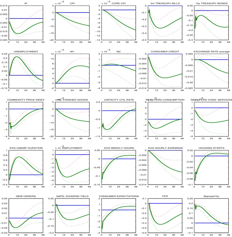
(17) shock. Note that a measure of the external finance premium is not required to enter in this recursive structure. Again, the impact response of the credit spread is equal to the standard deviation of the identified credit shock, which is function of the relevant factor loadings in Λ and the corresponding elements in the rotation matrix H.. 4. Results. In this section, we present the main empirical results from our two main FAVAR specifications. The next section provides more robustness results from additional specifications. We could in principle plot the impulse responses of all variables contained in the informational panel Xt but we will focus on a subset of economic and financial indicators of interest. In all cases, the impulse to the component of εt corresponding to the credit shock is of size 1. The lag order in VAR dynamics in (2) is set to 3. Finally, the 90% confidence intervals are computed using 5000 bootstrap replications.. 4.1. FAVAR 1 and monthly balanced panel. We estimate the first specification of the FAVAR using the monthly balanced panel. The recursive identification scheme, [πCP I , U R, F F R, B-spread], implies extracting four static factors from the data, Xt . Figure 2 plots the impulse responses of the level of key variables to the credit shock. On impact, the B-spread (lower right panel) rises by 19.2 basis points relative to its initial value. This unexpected increase in the external finance premium generates a significant and very persistent economic downturn, in line with the transmission channels discussed above. For example, industrial production (IP) falls little on impact but then by as much as 2% within the first 12 months, before returning to its initial level after 4 years. Employment falls by around 0.5% over the first year and remains significantly below the initial level for at least 3 years. Average weekly hours worked and capacity utilization also. 14.

(18) decrease, but they do fall significantly on impact. Real personal consumption falls significantly and persistently along with consumer credit, though the consumption decline is more muted (about 0.3% after a year) than that of production and consumer credit, in line with theories emphasizing the intertemporal smoothing of consumption. The labor market indicators such as the unemployment rate and average unemployment duration rise significantly for about 3 years, while employment and wages (average hourly earnings) decline. The price indices based on the CPI, core CPI, and PPI, show almost no change on impact and present a very persistent decline thereafter, settling four years later at a permanently lower level than would have obtained without the credit shock. Note that while our identification restriction prevents the CPI-based inflation to change contemporaneously with the credit shock, the responses of inflation based on the core CPI or the PPI are allowed to respond contemporaneously. The fact that they show no response on impact provides some comfort to our identifying assumption. The leading indicators, such as consumer expectations, new orders, housing starts, and commodity prices, all react negatively on impact, and remain below their initial level for at least a year following the credit shock. Similarly, 3-month and 5-year yields on Treasury securities fall markedly on impact and in years following the shock. While the Federal funds rate is prevented from declining on impact, by assumption, it does fall in the subsequent months, reaching a drop of about 40 basis points one year after the shock. The assumption of no contemporaneous change in the Federal funds rate could be justified by the fact that such changes occur mostly at pre-scheduled FOMC dates, and thus may not respond immediately to credit spread shocks. We will however assess below how empirically realistic such an assumption is by considering alternative identifying restrictions. Note finally, that as interest rates decrease the demand for monetary aggregate M1 increases, while M2 remains roughly unchanged. Some of these responses, in particular those involving leading indicators and interest. 15.

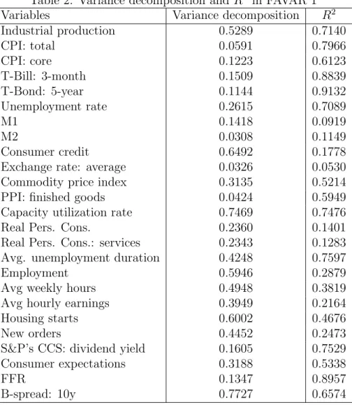
(19) rates, contrast sharply with those of GYZ, who assumed that no macroeconomic variable could respond on impact to credit shocks. Yet, even though long-term rates fall and thereby partially offset the adverse effects of the credit shock by stimulating consumption and investment, economic activity remains depressed following the negative credit shock. Indeed our estimate of the effect of the credit shock on industrial production is not too different from that of GYZ.9 Our arguably more realistic identifying assumptions allow us to obtain quantitatively reasonable responses of a large set of variables. This reinforces GYZ’s conclusion that disturbances to US credit markets can have an important impacts on economic activity. Table 2 shows the importance of credit shocks in explaining economic fluctuations during our 1959-2009 sample. The middle column reports for key macroeconomic series, xi,t , the contribution of the credit shock to the variance of the forecast error of the respective series at a 48-month horizon. Interestingly, the credit shock has important effects on many crucial variables: it explains more than 50% of the forecast error variance of industrial production, consumer credit, capacity utilization rate, labor market series, some leading indicators and credit spreads. Table 2 also shows that aggregate disturbances explain overall a large fraction of fluctuations in key economic time series. Indeed, the third column of Table 2 contains the fraction of the variability of each series explained by the common factors, i.e., the R2 obtained from 0. 0. the regression of xi,t on λi Ft for each indicator i, where λi denotes the i-th row of matrix Λ in equation (1). The common components explain a sizeable fraction of the variability in most of the indicators listed, especially for industrial production, prices, financial indicators, average unemployment duration, capacity utilization and consumer expectations, though variables such the exchange rate seem to be driven mostly by other factors. 9. GYZ find that industrial production falls by about one percent over a 24-month period following a shock corresponding to a 10-50 basis points increase in the credit spreads.. 16.

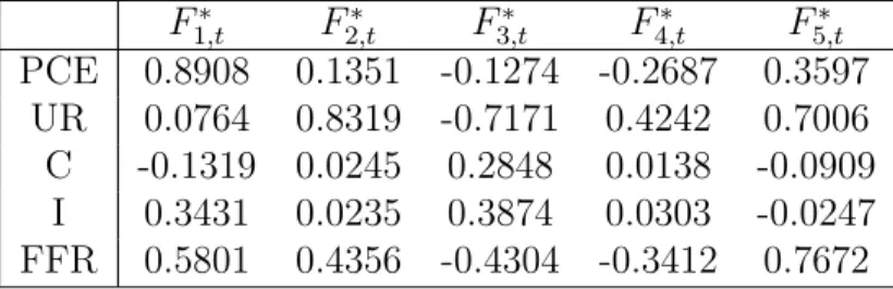
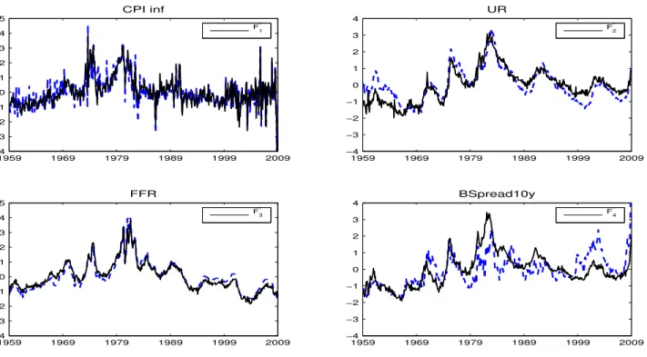
(20) 4.1.1. Interpretation of factors. While the common factors considered do capture an important dimension of the business cycle movements in most indicators, as just discussed, how can one interpret the common factors? Another interesting feature of our identification approach is that it allows us to obtain the rotation matrix H which can be used to interpret the estimated factors. Recall from Section 3.2, that structural shocks are a linear combination of residuals, εt = Het . Using this hypothesis, we can rewrite the system (1)-(2) in its structural form. Xt = Λ? Ft? + ut. (7). ? Ft? = Φ? (L)Ft−1 + εt. (8). where Ft? = HFt , Λ? = ΛH −1 , and Φ? (L) = HΦ(L)H −1 . Hence, given the estimates of ˆ Fˆt , associated with Ft and H, we can obtain an estimate of the structural factors, Fˆt? = H the structural shocks εt . Table 3 presents the correlation coefficients between the estimated rotated factors, Ft? , and the variables used in the recursive identification scheme. The factors ˆ and associated variables are plotted in Figure 3. The results reveal that the rotation by H yields estimated structural factors very close to the observed indicators used in the recursive identification scheme: the first rotated factor is highly correlated with πCP I , the second is related to the unemployment rate, the third to the Federal funds rate and the last to our credit spread measure.. 4.1.2. How important were credit spreads in the Great Recession?. Having estimated “structural” factors, it is now possible to use our model to evaluate the extent to which credit spreads contributed to the economic downturn in the Great Recession. To do so, we simulate our estimated model in structural form, excluding the credit shock, and compare the resulting simulated series to the actual data. In Figure 4, we plot the actual. 17.

(21) and simulated series of interest from 2007M1 to 2009M6, the date at which the recession officially ended.10 The data are simulated using the system (7)-(8) where the last element of εt is set to zero in the FAVAR 1 from 2007M1 to 2009M6, and the initial conditions for the factors are given by the estimated value of Ft∗ in 2006M12. Figure 4 reveals that credit shocks were important during the Great Recession for many real activity and price series. The simulation (indicated by black dashed lines) shows that a downturn in many activity and price indicators would have taken place even in the absence of credit spread shocks. In response to this downturn, short-term interest rates would have fallen. However a recovery would have been underway starting in late 2008, and short-term rates would have begun to normalize by early 2009. The jump in credit spreads, in particular in the Fall of 2008, was responsible for causing a much deeper recession and a collapse in many indicators. The simulation shows for example that credit spread shocks reduced industrial production and employment in mid-2009 by more than 20% and 7%, respectively, compared to the levels that would have obtained without credit spread shocks. Similarly, credit spread shocks are estimated to have increased the unemployment rate by more than 3 percentage points, and reduced the consumer price index by about 3%, by mid-2009. As a result, the Federal funds rate was lowered to near zero. These findings appear in line with Stock and Watson (2012) who point to exceptionally large shocks associated with financial disruptions and uncertainty in explaining the economic collapse during the Great Recession.. 4.2. FAVAR 2 and mixed-frequencies panel. To assess the robustness of the results discussed above, we consider an alternative identification scheme and incorporate additional data. Our second specification uses the mixedfrequencies monthly panel and impose the recursive identification based on the following 10. According to the NBER, the Great Recession lasted from December 2007 to June 2009.. 18.

(22) ordering [πP CE , U R, ∆C, ∆I, F F R]. As mentioned previously, the credit shock and the monetary policy shock are ordered respectively fourth and fifth in εt . An advantage of this specification compared to the FAVAR 1 is that it allows the Federal funds rate to respond contemporaneously to identified shocks to credit conditions. The latter shocks are assumed to cause a contemporaneous change in physical investment but no contemporaneous response of inflation based on the PCE deflator, unemployment, or real consumption. A potential downside of this specification, however, is that the identified shock to credit conditions is less directly related financial market data. The impulse responses to an unexpected disturbance to credit conditions are presented in Figure 5. The impact response of the B-spread is a little more than 20 basis points, i.e., a response similar to the one considered in FAVAR 1. In contrast to the previous specification, the Federal funds rate declines significantly on impact, now that its contemporaneous response is left unrestricted. This results in a large impact response of the 3-month Treasury bill yield and of the S&P composite common stock dividend yield. However, the impulse responses of other variables do not appear to differ much from those of the previous specification. Indeed, the unexpected increase in the external finance premium generates a significant and persistent economic slowdown and an associated large and persistent decline in price indexes. Industrial production, capacity utilization and employment present a significant downturn for about 18 months after the shock. The unemployment rate and the average unemployment duration both increase persistently, while employment and salary indicators decline. The leading indicators of economic activity — housing starts, new orders, and consumer expectations — react negatively and significantly on impact. Figure 6 displays the impulse responses of some monthly indicators constructed from the quarterly observed variables. These are GDP components and two price indexes. We can see that the GDP and PCE deflators decline in a persistent and significative fashion, though the responses of the other variables are less precise. However, we notice that after a small. 19.

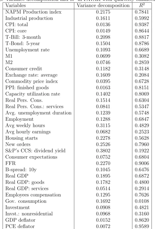
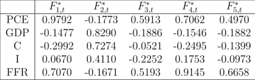
(23) positive impact response, most aggregates decline progressively. Table 4 reports the contribution of the credit shock to the variance of the forecast error in key indicators, as well as the R2 statistics measuring the importance of common factors in explaining fluctuations in these indicators. As for the FAVAR 1, the R2 statistics are fairly high for many indicators, suggesting that aggregate disturbances explain overall a large fraction of fluctuations in these economic time series. In the FAVAR 2, the credit shock still reveals important effects on many crucial variables. While the credit shock still explains a relatively large fraction of the variance of the forecast error of prices, financial indicators including Federal funds rate, the capacity utilization rate and consumer credit, it explains a somewhat smaller fraction for real economic activity measures than was the case in the FAVAR 1 specification. For instance, the credit shock accounts for 29% of the forecast error variance of industrial production and 40% of the forecast error variance of employment at the 48-month horizon.. 4.2.1. Interpretation of factors. As for the previous specification, we can check how the rotation matrix changes the correlation structure between the estimated factors and the economic indicators used in the recursive identification scheme. Table 5 contains the correlation coefficients and Figure 7 plots the rotated factors and the corresponding series. We find that the first structural factor is important for the price series and the second for unemployment rate. The third factor is related to the consumption series and negatively correlated with U R. The fourth factor is less correlated with identification variables, while the fifth factor is related to the Federal funds rate.. 20.

(24) 4.2.2. Effects of credit spreads in the Great Recession. Again, we can assess how important the estimated credit spreads were in deepening the downturn in the 2007-2009 period. Figures 8 and 9 compare actual data (solid blue lines) with the simulated series of interest (dashed black lines) for the period 2007M1 to 2009M6, using the system (7)-(8) and setting the shock to the credit conditions (i.e., the fourth element of εt ) to zero. As for the previous specification, Figures 8 and 9 show that credit shocks were important in deepening the Great Recession for most real activity and price series. For instance, they reduced industrial production and employment in mid-2009 by more than 10% and 4%, respectively. In comparison to the FAVAR 1 specification, however, the tightening in credit conditions had a somewhat smaller effect. The reason is that in the FAVAR 2 specification, the short-term interest rates would not have fallen enough, in the absence of credit shocks, to induce a rapid recovery.. 5. Further robustness analysis. To provide further robustness analysis of the results described above, we estimate several other FAVAR specifications, using among others only quarterly data, and considering alternative representations of the FAVAR model in which some factors are assumed to be observed.. 5.1. FAVAR with sign restrictions and a quarterly balanced panel. In this specification, we consider an updated version of balanced quarterly panel from Boivin and Giannoni (2006) containing 220 quarterly U.S. series for the same period, and identify the credit shock using a sign restrictions strategy. To obtain the initial orthogonalized innovations we start from the recursive structure on the indicators [πP CE , ∆GDP , ∆C, ∆I,. 21.

(25) F F R] entering the data set Xt which we assumes satisfies: Xt ' B ? (L)εt .. (9). Then, we generate an orthogonal matrix Q, using a QR decomposition, such that. ˜ ? (L)˜ Xt ' B εt , ˜ ? (L) ≡ B ? (L)Q and ε˜t ≡ Q0 εt . The following sign restrictions are imposed on the where B impact matrix B˜? (0): ∂(πP CE,t ) ≤ 0, ∂(εCS t ). ∂(∆GDPt ) ≤ 0, ∂(εCS t ). ∂(∆Ct ) ≤ 0, ∂(εCS t ). ∂(∆It ) ∂(∆Ct ) < . CS ∂(εt ) ∂(εCS t ). (10). Hence, we require that the impact responses of PCE inflation, and of the growth rates of real GDP, consumption and investment to a contractionary credit shock be non positive. The last restriction means that the investment (nonresidential) responds more than consumption. The results were obtained after simulating 10,000 orthogonal matrices. Among them, 924 were retained as they respected all the sign restrictions. The impulse responses computed with the median orthogonal matrix are presented with solid black lines in Figure 10, and all retained impulse responses are represented by the gray areas. The dynamic effects of the credit shock are similar to what we have observed in the previous specifications. The identified shock to credit conditions causes a sizeable economic downturn: production, employment, consumer credit, and prices decline, while the unemployment rate and average unemployment duration rise. Interest rates, housing starts, new orders, and the capacity utilization rate react negatively on impact, while credit spreads respond positively, as expected. However, compared to the previous monthly models, the effects of credit shocks appear less persistent.. 22.

(26) In Table 6 we present variance decomposition and R2 results. In contrast with previous approaches, the credit shock has a smaller effect on most of the variables. It explains between 20 and 30 percent of the forecast error in the quarterly NAPM production index, the Federal funds rate, and some leading indicators, but has a small effect on prices and monetary measures. The R2 results suggest that the extracted factors explain an important fraction of the variability in these series. Table 7 presents the correlation structure between rotated factors and the series used in the recursive identification. These are also plotted in Figure 11. The interpretation of structural factors is quite similar to the previous FAVAR 2 specification.. 5.2. FAVARs with observed factors. We now consider FAVAR models that include some observable factors in the transition equation along with the latent factors, as in Boivin, Bernanke and Eliasz (2005) and in Boivin, Giannoni and Stevanović (2009). The model is. X t = Λ F F t + Λ Y Yt + u t     Ft−1   Ft   + et ,   = Φ (L)  Yt−1 Yt. (11). . (12). where Ft contains K latent factors and Yt has M observable series. In case of the two-step estimation procedure, the issue is to separate the space spanned by observable and unobservable factors. We considered two alternative approaches.11 In either case, the identification 11. In the first approach, following Bernanke, Boivin and Eliasz (2005), Yt contains the Federal Funds Rate (F F R). As these authors, we split the sample into a block of ‘slow moving’ series that do not respond immediately to a shock on F F R, and another consisting of ‘fast moving’ variables that are not restricted. ˆ t , Yt ) be the K principal components The latent factors are obtained from the following steps: (i) Let C(F of Xt ; (ii) Let XtS be the subset of ‘slow moving’ variables. Let C ∗ (Ft ) be the K principal components of ˆ t , Yt ) − βˆY Yt where βˆY is obtained by least squares estimation of the regression XtS ; (iii) Define Fˆt = C(F ˆ t , Yt ) = βC C ∗ (Ft ) + βY Yt + at ; (iv) Get the loadings by regressing Xt on Fˆt and Yt . C(F In the second approach, following Boivin, Giannoni and Stevanović (2009), we estimate the latent factors through an iterative application of the principal components estimator. Starting from an initial estimate of. 23.

(27) of structural shocks is achieved by imposing a recursive structure on the VAR residuals in (12). In our context, Yt contains a proxy of the external finance premium and may contain other observable series. For each estimation procedure, we tried several specifications: • Yt contains only one of the credit spreads; • Yt contains a credit spread and the Federal funds rate, and considering different orderings in Yt ; • we include different numbers of latent factors in Ft . Overall, the results are very similar to those presented here. Each specification reveals a significant and persistent economic downturn following the credit shock, and depending on the identification procedure, the interest rates and leading indicators respond immediately to the shock. This reinforces our empirical evidence about the real effects of financial disturbances on economic activity.. 6. Relevance of Large Data Sets. Our analysis has so far considered the effects of credit shocks in FAVAR models that exploit information from large panels of data series. Besides the fact that FAVAR models yield a more complete picture of the effects of particular shocks on the economy, a key justification for using such models is that they have been shown to address a number of empirical puzzles obtained in analyses of empirical models (VARs) involving a small number of data series, especially in response to unanticipated monetary policy shocks. A natural question is thus whether information from large data sets is also relevant to properly characterize the response of credit shocks. To address this question, we compare our findings to those obtained from ˆ F,j and Ft , Ft0 which is the K first principal components of Xt : (i) Regress Xt on Fˆt0 and Yt to obtain Λ j Y,j Y,j ˆ ˜ ˆ ˆ ˜ Λ ; (ii) Compute Xt = Xt − Λ Yt ; (iii) Update Ft as the first K principal components of Xt . The main advantage of this procedure is that it does not rely on any temporal assumption between the observed factors and the informational panel. By construction, Fˆt is contemporaneously uncorrelated with Yt .. 24.

(28) standard structural VAR models. Our benchmark VAR model, similarly to Mueller (2007), has the following recursive ordering [πCP I , U R, F F R, 10yBS], where πCP I is the inflation rate calculated as the first difference in the log of the consumer price index (CPI), U R is again the unemployment rate, F F R is the Federal funds rate and 10yBS is the 10-year B-spread. Hence, inflation, unemployment and the Federal funds rate cannot respond in the same month to an unexpected increase in the credit spread. This identifying assumption is the same as the one adopted in the FAVAR 1, except that we now consider only a small set of data series. Figure 12 shows the effects of an unexpected increase in the 10-year B-spread that is such that the peak increase is 19.2 basis points, i.e., the same magnitude as the one considered in FAVAR 1. The shock causes again a significant and persistent increase in the unemployment rate, a fall in the price level, and a persistent reduction of the Federal funds rate. The responses are however smaller than the ones obtained in the context of the FAVAR that exploits information from a large data set. The peak response of the unemployment rate is less than 12 basis points in the VAR, compared to a response almost twice as large in the FAVAR 1. Similarly the decline in the CPI is more than double in the FAVAR 1 model than in the VAR. Since the small-scale VAR is a restricted version of the FAVAR 1, we view the VAR-based impulse responses as potentially more distorted than the ones obtained from the FAVAR. As the benchmark specification may be restrictive, we check the validity of our results by studying several alternative orderings and using credit spreads: 1yBS (1-year B-spread) and 10yAS (10-year A-spread). Table 8 lists all the SVAR models considered, and Figure 13 compares their results. This figure shows that the impulse responses are robust to different empirical measures of the external finance premium and to the ordering between monetary policy and credit shocks. While Figures 12–13 show the response of the unemployment rate, the CPI and the. 25.

(29) Federal funds rate to credit shocks, they do not allow us to determine how important credit shocks are in generating economic fluctuations. Table 9 reports the contribution of credit shocks to the total variance of these series. Based on small-scale structural VARs, the credit shocks appear to contribute again less to fluctuations in the CPI (less than 6% at most), and to the unemployment rate (around 20% at most) than is the case with the FAVAR model. One interesting finding is that the FAVAR impulse responses to credit shocks are qualitatively in line with the ones from the VARs, for the indicators included in the VAR. This suggests that after controlling for past inflation, unemployment and Federal funds rates, shocks to the credit market can be reasonably well captured by innovations in the credit spread. This contrasts with analyses of monetary policy shocks [e.g., Bernanke, Boivin and Eliasz (2005) and Boivin, Giannoni, Stevanovic (2009)] which show important qualitative differences between VAR and FAVAR responses of many variables. However, to obtain a correct gauge of the quantitative effect of credit shocks in explaining aggregate fluctuations also requires that the transmission mechanism of all shocks, including monetary shocks, be well specified. Given that relevant information is likely omitted in small-scale VARs, calculations based on the FAVAR models are likely to be more reliable. These results indicate that credit shocks are indeed much more important in explaining economic fluctuations than the small-scale VAR models suggest.. 7. Conclusion. In this paper, we have re-examined the evidence on the propagation mechanism of credit shocks to economic activity. The analysis has been done in a data-rich environment using several specifications of a structural factor model. The structural shocks were identified by imposing a minimal number of restrictions on the matrix of impact responses of several economic indicators. The common factors are shown to explain an important fraction of the variability in 26.

(30) observable variables and thus capture a sizeable dimension of the business cycle movements. Moreover, our identification approach allows us to recover underlying structural factors which have an interesting economic interpretation. A variance decomposition analysis suggests that credit shocks have important effects on several real activity measures, price indicators, leading indicators, and credit spreads. The results show that an unexpected increase of a measure of the external finance premium generates a statistically and economically significant economic downturn. This downturn is persistent and broad based, and results in a significant increase in the unemployment rate and a gradual decrease in price indices. It takes place despite a rapid and significant decline in interest rates. Leading indicators including interest rates and measures of confidence respond strongly and significantly on impact. Our identifying assumptions that leave unconstrained the contemporaneous responses of most indicators yield a more realistic picture of the effect of credit shocks on the economy than has been found to date, and provide valuable information about the transmission of these shocks. A simulation of the Great Recession period reveals that the jump in credit spreads, in particular in the Fall 2008, was responsible for causing a dramatic deepening of the recession. Finally, our results are largely robust to different data frequencies and identification schemes.. 27.

(31) References [1] Bai, J., and S. Ng (2006), “Confidence intervals for diffusion index forecasts and inference for factor-augmented regressions,” Econometrica 74: 1133–1150. [2] Bai, J., and S. Ng (2008), “Large Dimensional Factor Analysis,” Foundations and Trends in Econometrics 3(2): 89–163. [3] Bernanke, B.S. and M. Gertler (1995), “Inside the black box: The credit channel of monetary policy transmission,” Journal of Economic Perspectives 9: 27–48. [4] Bernanke, B.S., M. Gertler and S. Gilchrist (1999), “The Financial Accelerator in a Quantitative Business Cycle Framework,” in The Handbook of Macroeconomics, ed. by J.B. Taylor and M. Woodford, pp. 1341–1369. Elsevier Science B.V. Amsterdam. [5] Bernanke, B.S., J. Boivin and P. Eliasz (2005), “Measuring the effects of monetary policy: a factor-augmented vector autoregressive (FAVAR) approach,” Quarterly Journal of Economics 120: 387–422. [6] Boivin, J., Giannoni M.P. (2006), “DSGE Models in a Data-Rich Environment,” NBER working paper no. 12772. [7] Boivin, J., Giannoni M.P., and D. Stevanović (2009), “Monetary Transmission in a Small Open Economy: More Data, Fewer Puzzles,” manuscript, UQAM. [8] Christiano, L.J., M. Eichenbaum and C. Evans (2005), “Nominal Rigidities and the Dynamic Effect of a Shock to Monetary Policy,” Journal of Political Economy 113(1): 1–45. [9] Christiano, L.J., R. Motto and M. Rostagno (2003), “The Great Depression and the Friedman-Schwartz Hypothesis,” Journal of Money, Credit, and Banking 35(6): 1119– 1198. 28.

(32) [10] Christiano, L.J., R. Motto and M. Rostagno (2009), “Shocks, Structures, or Monetary Policies? The Euro Area and U.S. After 2001,” Journal of Economic Dynamics and Control 32: 2476–2506. [11] Christiano, L.J., R. Motto and M. Rostagno (2013), “Risk Shocks,” NBER working paper no. 18682, January. [12] Doz, C., D. Giannone, and L. Reichlin (2006), “A Quasi Maximum Likelihood Approach for Large Approximate Dynamic Factor Models,” ECB Working Paper 674. [13] Engle, R.F. and M.W. Watson (1981), “A one-factor multivariate time series model of metropolitan wage rates,” Journal of the American Statistical Association 76: 774–781. [14] Forni, M., D. Giannone, M. Lippi, L. Reichlin (2009), “Opening The Black Box: Structural Factor Models With Large Cross Sections,” Econometric Theory 25(05): 1319– 1347. [15] Gertler, M. and C.S. Lown (1999), “The Information in the High-Yield Bond Spread for the Business Cycle: Evidence and Some Implications,” Oxford Review of Economic Policy 15: 132–150. [16] Giannone, D., L. Reichlin and L. Sala (2004), “Monetary policy in real time,” NBER Macroeconomics Annual, 161–200. [17] Gilchrist, S., V. Yankov and E. Zakrajˇsek (2009), “Credit Market Shocks and Economic Fluctuations: Evidence From Corporate Bond and Stock Markets,” Journal of Monetary Economics 56: 471–493. [18] Gilchrist, S., A. Ortiz and E. Zakrajˇsek (2009), “Credit Risk and the Macroeconomy: Evidence From an Estimated DSGE Model,” Mimeo, Boston University.. 29.

(33) [19] Jungbacker, D. and S.J. Koopman (2008), “Likelihood-Based Analysis for Dynamic Factor Models,” manuscript, Tinbergen Institute. [20] Kilian, L. (1998), “Small-Sample Confidence Intervals for Impulse Response Functions,”Review of Economics and Statistics 80(2): 218–230. [21] Mueller, P. (2007), “Credit Spreads and Real Activity,”Mimeo, Columbia Business School. [22] Philippon, T. (2009), “The Bond Market’s Q,”Quarterly Journal of Economics, forthcoming. [23] Sargent, T.J. (1989). “Two Models of Measurements and the Investment Accelerator,”Journal of Political Economy 97: 251–287. [24] Smets, Frank, and Raf Wouters (2007), “Shocks and Frictions in US Business Cycles: A Bayesian DSGE Approach,” American Economic Review 97(3): 586-606. [25] Stock, J.H., and M.W. Watson (1989), “New indexes of coincident and leading economic indicators,” NBER Macroeconomics Annual, 351–393. [26] Stock, J.H., and M.W. Watson (2002a). “Forecasting Using Principal Components from a Large Number of Predictors,”Journal of the American Statistical Association 97: 1167–1179. [27] Stock, J.H., and M.W. Watson (2002b), “Macroeconomic Forecasting Using Diffusion Indexes,” Journal of Business and Economic Statistics 20: 147–162. [28] Stock, J.H., and M.W. Watson (2003), “Forecasting Output and Inflation: The Role of Asset Prices,” Journal of Economic Literature 41: 788–829. [29] Stock, J.H., and M.W. Watson (2005), “Implications of Dynamic Factor Models for VAR Analysis,” manuscript, Harvard University. 30.

(34) [30] Stock, J.H., and M.W. Watson (2012), “Disentangling the Channels of the 2007-2009 Recession,” NBER WP 18094.. Table 1: Proxies for the external finance premium FYAAAC FYBAAC FYGT1 FYGT10 FYFF 10Y B-spread 10Y A-spread 1Y B-spread. Series description BOND YIELD: MOODY’S AAA CORPORATE BOND YIELD: MOODY’S BAA CORPORATE INTEREST RATE: U.S.TREASURY CONST MATURITIES,1-YR. INTEREST RATE: U.S.TREASURY CONST MATURITIES,10-YR. INTEREST RATE: FEDERAL FUNDS (EFFECTIVE) Credit spreads FYBAAC-FYGT10 FYAAAC-FYGT10 FYBAAC-FYGT1. 31. Time span 1959M01-2009M06 1959M01-2009M06 1959M01-2009M06 1959M01-2009M06 1959M01-2009M06 1959M01-2009M06 1959M01-2009M06 1959M01-2009M06.

(35) Table 2: Variance decomposition and R2 in FAVAR Variables Variance decomposition Industrial production 0.5289 CPI: total 0.0591 CPI: core 0.1223 T-Bill: 3-month 0.1509 T-Bond: 5-year 0.1144 Unemployment rate 0.2615 M1 0.1418 M2 0.0308 Consumer credit 0.6492 Exchange rate: average 0.0326 Commodity price index 0.3135 PPI: finished goods 0.0424 Capacity utilization rate 0.7469 Real Pers. Cons. 0.2360 Real Pers. Cons.: services 0.2343 Avg. unemployment duration 0.4248 Employment 0.5946 Avg weekly hours 0.4948 Avg hourly earnings 0.3949 Housing starts 0.6002 New orders 0.4452 S&P’s CCS: dividend yield 0.1605 Consumer expectations 0.3188 FFR 0.1347 B-spread: 10y 0.7727. 1 R2 0.7140 0.7966 0.6123 0.8839 0.9132 0.7089 0.0919 0.1149 0.1778 0.0530 0.5214 0.5949 0.7476 0.1401 0.1283 0.7597 0.2879 0.3819 0.2164 0.4676 0.2473 0.7529 0.5338 0.8957 0.6574. Notes: The second column reports for key macroeconomic series, xi,t , the contribution of the credit shock to the variance of the forecast error of the respective series at a 48-month horizon. The third column contains the fraction of the variability 0. of this series explained by the common factors, i.e., the R2 obtained from the regression of xi,t on λi Ft for each indicator i, 0. where λi denotes the i-th row of matrix Λ in equation (1).. Table 3: Correlation between rotated factors and variables in recursive identification in FAVAR 1 ∗ ∗ ∗ ∗ F1,t F2,t F3,t F4,t CPI 0.8925 0.2935 0.4822 0.1220 UR -0.0135 0.7906 -0.1070 0.7752 FFR 0.7282 0.6328 0.7091 0.4062 Bspread -0.1529 0.4996 -0.4542 0.7073. 32.

(36) Table 4: Variance decomposition and R2 in FAVAR Variables Variance decomposition Industrial production 0.2929 CPI: total 0.5139 CPI: core 0.5656 T-Bill: 3-month 0.6723 T-Bond: 5-year 0.6611 Unemployment rate 0.1915 M1 0.1601 M2 0.1899 Consumer credit 0.4470 Exchange rate: average 0.0941 Commodity price index 0.7903 PPI: finished goods 0.5114 Capacity utilization rate 0.7220 Real Pers. Cons. 0.0559 Real Pers. Cons.: services 0.1930 Avg. unemployment duration 0.3727 Employment 0.3980 Avg weekly hours 0.2261 Avg hourly earnings 0.4290 Housing starts 0.4582 New orders 0.2519 S&P’s CCS: dividend yield 0.5861 Consumer expectations 0.1652 FFR 0.6016 B-spread: 10y 0.7096 Real GDP 0.0737 Real GDP: goods 0.0890 Real GDP: services 0.0518 Employees compensation 0.0641 Gov. consumption 0.1032 Investment 0.0926 Invst.: nonresidential 0.0714 GDP deflator 0.1940 PCE deflator 0.1302. 2 R2 0.7313 0.6263 0.6211 0.8640 0.8948 0.6946 0.1090 0.0323 0.1893 0.0270 0.4731 0.3077 0.7405 0.3819 0.1086 0.6242 0.3037 0.3015 0.3364 0.4329 0.2500 0.6147 0.5088 0.8802 0.6416 0.9338 0.8860 0.8769 0.8812 0.6009 0.8599 0.9012 0.6547 0.7935. Notes: The second column reports for key macroeconomic series, xi,t , the contribution of the credit shock to the variance of the forecast error of the respective series at a 48-month horizon. The third column contains the fraction of the variability 0. of this series explained by the common factors, i.e., the R2 obtained from the regression of xi,t on λi Ft for each indicator i, 0. where λi denotes the i-th row of matrix Λ in equation (1).. 33.

(37) Table 5: Correlation between rotated factors and variables in recursive identification in FAVAR 2 ∗ ∗ ∗ ∗ ∗ F1,t F2,t F3,t F4,t F5,t PCE 0.8908 0.1351 -0.1274 -0.2687 0.3597 UR 0.0764 0.8319 -0.7171 0.4242 0.7006 C -0.1319 0.0245 0.2848 0.0138 -0.0909 I 0.3431 0.0235 0.3874 0.0303 -0.0247 FFR 0.5801 0.4356 -0.4304 -0.3412 0.7672. 34.

(38) Table 6: Variance decomposition and R2 in FAVAR with quarterly balanced panel Variables Variance decomposition R2 NAPM Production index 0.2175 0.7841 Industrial production 0.1611 0.5992 CPI: total 0.0136 0.9387 CPI: core 0.0149 0.8644 T-Bill: 3-month 0.2098 0.8817 T-Bond: 5-year 0.1504 0.8786 Unemployment rate 0.1093 0.6689 M1 0.0699 0.3082 M2 0.0746 0.2859 Consumer credit 0.1182 0.3148 Exchange rate: average 0.1609 0.2084 Commodity price index 0.0395 0.6728 PPI: finished goods 0.0163 0.8151 Capacity utilization rate 0.1402 0.8069 Real Pers. Cons. 0.1514 0.6304 Real Pers. Cons.: services 0.0841 0.5347 Avg. unemployment duration 0.1239 0.5748 Employment 0.1288 0.6847 Avg weekly hours 0.3115 0.4829 Avg hourly earnings 0.0682 0.2523 Housing starts 0.2278 0.5628 New orders 0.2526 0.7960 S&P’s CCS: dividend yield 0.3802 0.1922 Consumer expectations 0.0752 0.6804 FFR 0.2270 0.9006 B-spread: 10y 0.1045 0.6476 Real GDP 0.1895 0.6872 Real GDP: goods 0.1782 0.4800 Real GDP: services 0.0514 0.2914 Employees compensation 0.1295 0.7626 Gov. consumption 0.1692 0.0108 Investment 0.0908 0.4821 Invst.: nonresidential 0.0968 0.3160 GDP deflator 0.0152 0.8620 PCE deflator 0.0072 0.9589 Notes: The second column reports for key macroeconomic series, xi,t , the contribution of the credit shock to the variance of the forecast error of the respective series at a 16-quarter horizon. The third column contains the fraction of the variability 0. of this series explained by the common factors, i.e., the R2 obtained from the regression of xi,t on λi Ft for each indicator i, 0. where λi denotes the i-th row of matrix Λ in equation (1).. 35.

(39) Table 7: Correlation between rotated factors and identification variables in FAVAR with quarterly balanced panel ∗ ∗ ∗ ∗ ∗ F5,t F4,t F3,t F2,t F1,t PCE 0.9792 -0.1773 0.5913 0.7062 0.4970 GDP -0.1477 0.8290 -0.1886 -0.1546 -0.1882 C -0.2992 0.7274 -0.0521 -0.2495 -0.1399 I 0.0670 0.4110 -0.2252 0.1753 -0.0973 FFR 0.7070 -0.1671 0.5193 0.9145 0.6658. Table 8: VAR models used to study effects and identification of financial shock Models Wald causaility ordering Benchmark [πt , U Rt , F F Rt , 10yBSt ] Model 1 [πt , U Rt , 10yBSt , F F Rt ] Model 2 [πt , U Rt , F F Rt , 1yBSt ] Model 3 [πt , U Rt , F F Rt , 10yASt ]. Table 9: Variance decomposition: contribution of the credit shock Variables Benchmark Model 1 Model 2 Model 3 CPI 0.0467 0.0569 0.0227 0.0322 Unemployment rate 0.1945 0.1694 0.0477 0.0933 FFR 0.1055 0.1572 0.0882 0.0778 B-spread: 10y 0.9156 0.8968 B-spread: 1y 0.6069 A-spread: 10y 0.9437. 36.

(40) Figure 1: Measures of the external finance premium and unemployment Notes: The figure shows several measures of credit spreads (defined in Table 1) and the unemployment rate.. 37.

(41) −3 x 10. IP 0.015. −3 CORE CPI x 10. CPI. 5. 3m TREASURY BILLS. 2. 0.01. 10y TREASURY BONDS. 0. 0.05. 0 0. 0.005 0. 0 −0.1. −2. −0.05. −4. −5. −0.005. −0.2. −0.1. −6 −10. −0.01 −0.015. −8. −0.2. −10. −15. −0.02. −0.15. −0.3 −0.4. −0.25. −12. −0.025. −20 0. 12. 24. 36. 48. −14 0. 12. −3 x 10. UNEMPLOYMENT. 24. 36. 48. −0.5 0. 12. −3 x 10. M1. 24. 36. 48. M2. 12. 2. 0. 0.2. 10. 1. −0.002. 8. 0.1. 12. 24. 36. 48. 0. CONSUMER CREDIT. 0.25. 0.15. −0.3 0. 6. 0 −0.005 −0.01. −0.008 −2. 2. −0.015. −0.01. −0.1. 0. −3. −0.012. −0.02. −0.15. −2. −4. −0.014. −0.025. 0. 12. 24. 36. 48. 0. 12. 24. 36. 48. 0. −3 x PPI: 10 FINISHED GOODS. COMMODITY PRICE INDEX 1. 5. 0. 0. −1. −5. −2. −10. −3. −15. −4. −20. 12. 24. 36. 48. 0. 12. 24. 36. 48. −1.5 12. 24. 36. 48. 0. 12. 24. 36. −0.4. −7 0. 12. 24. 36. 48. −4. 48. −5 12. 24. 36. 48. 0. 12. 24. 36. 48. HOUSING STARTS 0.02 0. −0.004. −0.02 −0.04 −0.06. −0.01. −0.1. −0.08. −0.012 −0.15 12. 24. 36. 48. 0.03. −0.014 0. 12. 24. 36. 48. CONSUMER EXPECTATIONS 2 1. 0 0.02. 0. −0.1. 36. −0.008. S&PS: DIVIDEND YIELD. −0.05. 24. −0.006. 0.05. 0. −3. −4. −0.05. 0. 0.01. −2. −0.002. NEW ORDERS 0.04. −2. AVG HOURLY EARNINGS. 0. −5 −6. 0. 0. −4. 0. 0 −1. AVG WEEKLY HOURS. −3. −0.2. 12. −3 REAL x 10PERS CONS: SERVICES 1. 2. 0. 0.05. −2. 0.2. 0. 4. 48. 0. 0.4. 48. −6. −3 x 10 EMPLOYMENT. −1. 0.6. 36. −1. 1. 0.8. 24. 0. 0. AVG UNEMP DURATION 1. 12. −3 REAL x 10 PERS CONSUMPTION 6. CAPACITY UTIL RATE 0.5. −0.5. 0. 48. EXCHANGE RATE average. −1 4. −0.05. 36. −0.006. 0.05 0. 24. 0.005. −0.004. 0. 12. −0.1 0. 12. 24. 36. 48. 0. FFR. 12. 24. 36. 48. Bspread10y. 0.1. 0.25. 0. 0.2. −0.1. 0.15. −0.2. 0.1. −0.3. 0.05. −1 −2. −0.01 −0.15. −3. −0.02 −0.03. −0.2 0. 12. 24. 36. 48. −4 0. 12. 24. 36. 48. −0.4. 0. −0.5. −0.05. −0.6 0. 12. 24. 36. 48. −0.1 0. 12. 24. 36. 48. 0. 12. 24. Figure 2: Dynamic responses of monthly variables to credit shock in FAVAR 1. Notes: The figure plots the impulse responses of the level of key variables to the credit shock identified through the recursive identification scheme, [πCP I , U R, F F R, B-spread], where the credit shock is ordered last. The dotted lines indicate the 90% confidence intervals computed using 5000 bootstrap replications.. 38. 36. 48.

(42) CPI inf. UR. 5. 4. F*1. 4. F*2. 3. 3. 2. 2. 1. 1 0 0 −1. −1. −2. −2. −3. −3 −4 1959. 1969. 1979. 1989. 1999. −4 1959. 2009. 1969. FFR. 1979. 1989. 1999. 2009. BSpread10y. 5. 4. F*3. 4. F*4. 3. 3. 2. 2. 1. 1 0 0 −1. −1. −2. −2. −3. −3 −4 1959. 1969. 1979. 1989. 1999. −4 1959. 2009. 1969. 1979. 1989. 1999. 2009. Figure 3: Rotated factors and variables used in recursive identification in FAVAR 1. Notes: The figure plots the estimated structural factors and the variables in the recursive identification scheme, [πCP I , UR, FFR, B-spread].. 39.