Publisher’s version / Version de l'éditeur:
Canadian Hydraulics Centre. Technical Report, 2001-12
READ THESE TERMS AND CONDITIONS CAREFULLY BEFORE USING THIS WEBSITE. https://nrc-publications.canada.ca/eng/copyright
Vous avez des questions? Nous pouvons vous aider. Pour communiquer directement avec un auteur, consultez la
première page de la revue dans laquelle son article a été publié afin de trouver ses coordonnées. Si vous n’arrivez pas à les repérer, communiquez avec nous à [email protected].
Questions? Contact the NRC Publications Archive team at
[email protected]. If you wish to email the authors directly, please see the first page of the publication for their contact information.
NRC Publications Archive
Archives des publications du CNRC
For the publisher’s version, please access the DOI link below./ Pour consulter la version de l’éditeur, utilisez le lien DOI ci-dessous.
https://doi.org/10.4224/12340994
Access and use of this website and the material on it are subject to the Terms and Conditions set forth at
Ice decay and the ice regime system Timco, G. W.; Johnston, M.; Kubat, I.
https://publications-cnrc.canada.ca/fra/droits
L’accès à ce site Web et l’utilisation de son contenu sont assujettis aux conditions présentées dans le site
LISEZ CES CONDITIONS ATTENTIVEMENT AVANT D’UTILISER CE SITE WEB.
NRC Publications Record / Notice d'Archives des publications de CNRC:
https://nrc-publications.canada.ca/eng/view/object/?id=5081890e-146a-4a9f-a82c-2c70019b0329 https://publications-cnrc.canada.ca/fra/voir/objet/?id=5081890e-146a-4a9f-a82c-2c70019b0329
TP 13871 E
Ice Decay and the Ice Regime System
G.W. Timco, M. Johnston and I. Kubat Canadian Hydraulics Centre National Research Council of Canada
Ottawa, Ont. K1A 0R6 Canada
Technical Report HYD-TR-070
ABSTRACT
The Canadian Ice Regime System takes into account the decay of sea ice by allowing the addition of +1 to the Ice Multiplier for ice that is deemed to be decayed at the “rotten” stage. This report examines this approach based on an analysis of the strength of both first-year sea ice and multi-year sea ice, and the damage statistics for Arctic vessels. The analysis shows that there is no quantitative scientific basis for the current approach of taking into account the decay of sea ice in the Ice Regime System. The report provides a detailed discussion of the analysis with recommendations that (1) the decay of sea ice should be recast in terms of the strength of ice; (2) the summer bonus for reduced ice strength should be given once the ambient air temperature has been above 0°C for one month; (3) an analysis should be performed to define a similar criterion to be used during the growth (autumn) season; and (4) there should be no bonus for decayed multi-year ice.
TABLE OF CONTENTS ABSTRACT ___________________________________________________________ 1 TABLE OF CONTENTS _________________________________________________ 3 LIST OF FIGURES_____________________________________________________ 4 LIST OF TABLES ______________________________________________________ 4 1.0 INTRODUCTION ________________________________________________ 5 2.0 FIRST-YEAR SEA ICE____________________________________________ 8 2.1 Growth of Sea Ice ______________________________________________ 8 2.2 Ice Salinity ____________________________________________________ 8 2.3 Brine Volume and Total Porosity ________________________________ 10 2.4 Flexural Strength _____________________________________________ 11 2.5 Internal Processes within Sea Ice ________________________________ 12 2.6 Changes in Flexural Strength: Case Study_________________________ 13 2.7 Ice Borehole Strength __________________________________________ 15 2.8 Decay Process in First-Year Sea Ice ______________________________ 17 2.9 Ice Strength and Stages of Decay ________________________________ 19 3.0 MULTI-YEAR AND SECOND-YEAR ICE ___________________________ 21 3.1 Strength of Multi-year Ice ______________________________________ 21 3.2 Decay Process in Multi-year Ice _________________________________ 22 3.3 Decay of Multi-year Ice and the Ice Regime System _________________ 23 4.0 SHIP DAMAGE IN THE CANADIAN ARCTIC_______________________ 24 5.0 FIRST-YEAR ICE DECAY AND THE ICE REGIME SYSTEM__________ 26 6.0 SUMMARY AND RECOMMENDATIONS ___________________________ 28 7.0 REFERENCES _________________________________________________ 29
HYD-TR-070 Page 4
LIST OF FIGURES
Figure 1: Ice salinity versus ice thickness for cold first-year sea ice... 9 Figure 2: Flexural strength versus the square root of the brine volume for first-year sea ice... 11 Figure 3: Flexural strength and ice measurements used in the calculation ... 14 Figure 4: Ice borehole strength for two measurement seasons... 16 Figure 5: Typical, mid-winter ice borehole strength and strengths from decay work
... 17 Figure 6: Comparison of ice borehole strength and calculated flexural strength .... 18 Figure 7: Comparison of normalized ice borehole strength and calculated flexural
strength ... 19 Figure 8: Relation between decay of ice strength and air temperature... 20 Figure 9: Borehole jack strength as a function of ice temperature for multi-year ice.
... 22 Figure 10: Vessel traffic in the Canadian Arctic by month for the 1996 calendar
year (data from Mariport Inc.) ... 24 Figure 11: Histogram showing the number of damage Events in the Arctic for each
month... 25
LIST OF TABLES
Ice Decay and the Ice Regime System
1.0 INTRODUCTION
Navigation in Canadian waters north of 60°N latitude is regulated by the Arctic Shipping Pollution Prevention Regulations (ASPPR). These regulations include the date Table in Schedule VIII and the Shipping Safety Control Zones Order, made under the Arctic Waters Pollution Prevention Act. Both of these are combined to form the “Zone/Date System” matrix that gives entry and exit dates for various ship types and classes. It is a rigid system with little room for exceptions. It is based on the premise that nature consistently follows a regular pattern year after year.
Transport Canada, in consultation with stakeholders, has made extensive revisions to the Arctic Shipping Pollution Prevention Regulations (ASPPR 1989; Canadian Gazette 1996; AIRSS 1996). These changes, introduced only outside the zone-date system, were designed to reduce the risk of structural damage in ships which could lead to the release of pollution into the environment, yet provide the necessary flexibility to shipowners by making use of actual ice conditions, as seen by the Master. In this new system, an "Ice Regime", which is a region of generally consistent ice conditions, is defined at the time the vessel enters that specific geographic region, or it is defined in advance for planning and design purposes. The Arctic Ice Regime Shipping System (AIRSS) is based on a simple arithmetic calculation that produces an “Ice Numeral” that combines the ice regime and the vessel’s ability to navigate safely in that region. The Ice Numeral (IN) is based on the quantity of hazardous ice with respect to the ASPPR classification of the vessel (see Table 1). The Ice Numeral is calculated from
.... ] [ ] [ + + = CaxIMa CbxIMb IN (1) where IN = Ice Numeral
Ca = Concentration in tenths of ice type “a”
IMa = Ice Multiplier for ice type “a” (from Table 1)
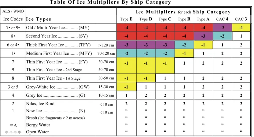
The term on the right hand side of the equation (a, b, c, etc.) is repeated for as many ice types as may be present, including open water. The values of the Ice Multipliers are adjusted to take into account the decay or ridging of the ice by respectively adding or subtracting a correction of 1 to the Ice Multiplier (see Table 1).
The Ice Numeral is therefore unique to the particular ice regime and ship operating within its boundaries.
HYD -TR -070 Page 6 Table 1
Table of Ice Multipliers for AIRSS
T a b l e O f I c e M u l t i p l i e r s B y S h i p C a t e g o r y
AES / WMO I c e M u l t i p l i e r s for each S h i p C a t e g o r y
Ice Codes I c e T y p e s Type E Type D Type C Type B Type A CAC 4 CAC 3
7• or 9• Old / Multi-Year Ice... (MY) -4 -4 -4 -4 -4 -3 -1
8• Second Year Ice ... (SY) -4 -4 -4 -4 -3 -2 1
6 or 4• Thick First Year Ice ... (TFY) > 120 cm -3 -3 -3 -2 -1 1 2
1• Medium First Year Ice ... (MFY) 70-120 cm -2 -2 -2 -1 1 2 2
7 Thin First Year Ice ... (FY) 30-70 cm -1 -1 -1 1 2 2 2
9 Thin First Year Ice - 2nd Stage 50-70 cm
8 Thin First Year Ice - 1st Stage 30-50 cm -1 -1 1 1 2 2 2
3 or 5 Grey-White Ice... (GW) 15-30 cm -1 1 1 1 2 2 2 4 Grey Ice... (G) 10-15 cm 1 2 2 2 2 2 2 2 1 ð∆ °°°°
Nilas, Ice Rind
New Ice ... (N) Brash (ice fragments < 2 m across)
Bergy Water Open Water < 10 cm < 10 cm 2 “ “ “ “ 2 “ “ “ “ 2 “ “ “ “ 2 “ “ “ “ 2 “ “ “ “ 2 “ “ “ “ 2 “ “ “ “
Notes: Decayed Ice: For the following ice types: MY, SY, TFY, and MFY that are ‘decayed’, add 1 to the Ice Multiplier.
Ridged Ice: For floes of ice that are over 3/10ths ‘Ridged’ and in an overall concentration that is greater than 6/10ths, subtract 1 from the Ice Multiplier.
The ASPPR deals with vessels that are designed to operate in severe ice conditions for transit and icebreaking (CAC class) as well as vessels designed to operate in more moderate first-year ice conditions (Type vessels). The System determines whether or not a given vessel should proceed through that particular ice regime. If the Ice Numeral is negative, the ship is not allowed to proceed. However, if the Ice Numeral is zero or positive, the ship is allowed to proceed into the ice regime. Responsibility to plan the route, identify the ice, and carry out this numeric calculation rests with the Ice Navigator who could be the Master or Officer of the Watch. Due care and attention of the mariner, including avoidance of hazards, is vital to the successful application of the Ice Regime System. Authority by the Regulator (Pollution Prevention Officer) to direct ships in danger, or during an emergency, remains unchanged.
At the present time, there is only partial application of the ice regime system, exclusively outside of the “zone-date” system.
Credibility of the new system has wide implications, not only for ship safety and pollution prevention, but also in lowering ship insurance rates and predicting ship performance. Therefore, there is a need to establish a scientific basis for the system. To this end, Transport Canada approached the Canadian Hydraulics Centre of the National Research Council of Canada (CHC/NRC) in Ottawa to assist them in developing a methodology for establishing a scientific basis for AIRSS. Considerable progress has been made in addressing the scientific basis (see Timco and Kubat (2001) for a recent update).
One important aspect of the Ice Regime System (IRS) is the decay of the sea ice. As noted in Table 1, an additional integer value is added to the Ice Multiplier if specific types of sea ice are decayed. The IRS allows the addition of one to the Ice Multiplier if the multi-year (MY) ice, second-year (SY) ice, thick year (TFY) ice or medium first-year (MFY) ice is decayed. No allowance is made for decay in thinner ice. This modification can significantly increase the Ice Numeral for decayed ice regimes.
This modification for decay was originally done on an “ad hoc” basis with no scientific evidence established for it. Further, there is no accepted definition of ice decay. Because of this, Transport Canada has asked the CHC/NRC to review this question. In this report, the strength of sea ice is reviewed with an eye towards the decay process. This is done for both first-year sea ice and older, multi-year and second-year sea ice. Following that, the ship damage events in the Arctic are reviewed to look for a correlation between sea ice decay and (less) damage. This is followed by some recommendations for the approach that should be taken for considering the decay of sea ice in the Ice Regime System.
HYD-TR-070 Page 8
2.0 FIRST-YEAR SEA ICE
2.1 Growth of Sea Ice
Sea ice is a complex material which is composed of solid ice, brine, air and, depending upon the temperature, solid salts. Ice growth mechanisms can produce several different grain structures, depending upon the prevailing conditions. The details of the ice microstructure influence significantly the mechanical and physical properties of the ice. In general, sea ice is a mix of grain structures including S2 columnar, granular, frazil and discontinuous columnar. The classic picture of sea ice structure (see e.g., Weeks and Ackley 1982) shows an upper granular structure overlying a S2 columnar structure. Although this type of composite structure is prevalent in land-fast ice in Arctic regions, it is certainly not universal. In many cases, especially in pack ice, there can be considerable "banding" of alternating layers of columnar and granular ice, often with discontinuous columnar ice. Moreover, in certain areas, considerable frazil ice has been observed on the bottom of an ice sheet. Thus the overall structure of the ice can be quite variable. When the ice grows, it traps some of the salt that is present in the seawater. The amount of salt that is trapped in the growing ice sheet is affected by several factors. Typically first-year sea ice has salinity in the range of 4 to 6 parts per thousand (‰) salt. This is lower than the salinity of seawater, which is typically 35 ‰. The brine, air and solid salts are usually trapped at sub-grain boundaries between a mostly pure ice lattice. Also, because a temperature gradient exists, the upper surface temperature is close to the ambient air temperature, and the lower surface temperature is at the freezing point (usually -1.8°C for sea ice). Because there are a number of salts in the ice, the phase relationship with temperature is multifarious (see e.g., Weeks and Ackley 1982). All of these factors make understanding and charactering sea ice extremely difficult.
2.2 Ice Salinity
For sea ice, the salinity (Si) is usually expressed as the fraction by weight of the salts
contained in a unit mass. It is usually quoted as a ratio of grams per kilogram of seawater, that is, in parts per thousand (‰ or ppt). In sea ice there is usually some salinity variation with depth in the ice sheet. This depth dependence of the salinity changes throughout the winter as the salt within the ice migrates downward through the ice. There can be, however, marked salinity variations even within a small sample. In many cases, therefore, the average value of a salinity profile is used as a first approximation of salinity for an ice sheet.
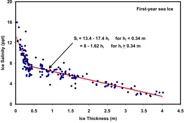
In collating information on sea ice from a wide number of sources, Cox and Weeks (1974) found that the average salinity of a cold ice sheet could be related to the thickness of the ice (hi). Figure 1 shows a plot of the average ice salinity versus ice thickness for a
large number of measurements on sea ice sampled during the growth season. The graph gives the original data of Cox and Weeks along with some more recent data from Frederking and Timco, Sinha and Nakawo, and Frederking. The data were collected from
cores from all parts of the Arctic including the Beaufort Sea, Bering Sea, Labrador, Eclipse Sound and Strathcona Sound. From Figure 1 it appears that a reasonable representation of the ice salinity for a given ice thickness hi can be expressed as (from
Timco and Frederking 1990):
; 34 . 0 4 . 17 4 . 13 h for h m Si = − i i ≤ ; 34 . 0 62 . 1 0 . 8 h for h m Si = − i i ≥ (2)
This approach assumes that there is no salinity variation with depth through the ice sheet, which is a reasonable first approximation for sea ice. Equation (2) gives the average salinity of sea ice as a function of the ice thickness. As evidenced in Figure 1, there is a good fit of the equations to the data. The change in salinity with thickness reflects the drainage of the brine during the year, and the fact that slower growth rates trap less salt in the ice sheet. With thicker ice, the growth rate is substantially lower than that for a thin (usually snowless) ice sheet in the early winter. All of these factors affect the strength of the ice. 0 4 8 12 16 20 0 0.5 1 1.5 2 2.5 3 3.5 4 4.5 Ice Thickness (m) Ice Salinity (ppt) Si = 13.4 - 17.4 hi for hi < 0.34 m = 8 - 1.62 hi for hi > 0.34 m
First-year sea Ice
HYD-TR-070 Page 10
2.3 Brine Volume and Total Porosity
Historically sea ice has been analyzed in terms of the "brine volume" in the ice. The brine volume represents the amount of liquid brine in the host ice matrix. The determination of the brine volume integrates the influence of both temperature and salinity. The brine volume of the ice is related to the temperature (Ti ) of the ice, the salinity (Si ) of the ice
and the types of salts present. For sea ice, the brine volume can be determined from the Frankenstein and Garner (1967) Equation:
+ = 49.185 0.532 i i b T S υ (3)
where -0.5°C ≥ Ti ≥ -22.9°C; or from the Cox and Weeks (1982) equation: ) ( /F1 T Si i b ρ υ = (4)
where ρi is the bulk ice density, and
F1(Ti ) = - 4.732 - 22.45 Ti - 0.6397 Ti2 - 0.01074 Ti3
for - 2 ≥ Ti≥ - 22.9
= 9899 + 1309 Ti + 55.27 Ti2 + 0.716 Ti3
for - 22.9 ≥ Ti≥ - 30
Although the latter is more accurate, the former provides a reasonable estimate of the brine volume. The brine volume is usually quoted in terms of the volume in parts per thousand, similar to the salinity. Alternatively, it can be expressed as a volume fraction. (For example, a brine volume of 20 ‰ is equivalent to a brine volume fraction of 0.020). Knowledge of the brine volume for sea ice is useful on its own. However, in addition to the liquid brine in the ice, air is present in the ice. In certain instances (especially where brine drainage occurs) the air volume can be significant. For this reason it is usually better to express the porosity of the ice as the total porosity (i.e. brine plus air). For this, the total porosity (νT) of the ice is expressed as
νT = νb + νa (5)
where νb is the relative brine volume and νa is the relative air volume. Cox and Weeks
(1982) developed equations to calculate the total porosity. To do this, the bulk ice density must be known accurately. Since this is a property that is not usually known due to the difficulty of an accurate measurement, the following discussion will be related only to the brine volume.
2.4 Flexural Strength
Several researchers have attempted to relate the strength of sea ice to the brine volume or total porosity of the ice. There is a good reason for this. It is generally assumed that as the total porosity in the ice increases, the strength should decrease since there is less "solid ice" that has to be broken. Timco and O’Brien (1994) have done the most comprehensive analysis of the flexural strength of ice. They compiled a database of over 2500 reported measurements on the flexural strength of freshwater ice and sea ice. For this data set, approximately 1000 tests were performed on sea ice. Timco and O’Brien (1994) showed that the data for first-year sea ice could be described by:
) * 88 . 5 ( exp 76 . 1 b f υ σ = − (6)
where σ f is the flexural strength of the ice and the brine volume (νb) is expressed as a
brine volume fraction. This relationship is shown with the data in Figure 2.
0 0.5 1 1.5 2 0 0.1 0.2 0.3 0.4 0.5 0.6
Square Root of Brine Volume (νb)1/2
Flexural Strength (MPa)
First-year Sea Ice
Average value for freshwater ice
σf = 1.76 exp [-5.88*sqrt(νb)]
Figure 2: Flexural strength versus the square root of the brine volume for first-year sea ice.
There are several things to note from this figure:
• The value of 1.76 MPa for zero brine volume is in excellent agreement with the average strength (1.73 MPa) measured for freshwater ice.
• The general scatter in the data increases with decreasing brine volume. This is a reflection of the fact that, at low brine volumes, the ice is much more brittle. The
HYD-TR-070 Page 12
range of scatter approaches that measured for freshwater ice. This type of scatter is characteristic of a brittle material. It is natural scatter.
• This equation is the most comprehensive equation for flexural strength to date. There have been a few other equations proposed to relate strength and brine volume but these have been based on substantially fewer data points, and data that extended over a very limited range. In other words, the other equations are valid over only a small brine volume range. The wider range of this equation represents these other equations very well in the ranges where they are valid.
• The data for the equation was compiled from a large number of investigators, and from a variety of geographic locations, in both polar and temperate climates. Therefore it should be quite representative of the flexural strength of sea ice in most regions.
• The brine volume used to represent the ice beam for any test was taken to be the average brine volume, determined from the average temperature and salinity of the beam. Thus, to calculate the flexural strength, it is only necessary to know the average temperature and salinity of the ice.
In summary, the fact that a very large number of data points have been used in this analysis, the excellent agreement with the flexural strength of freshwater ice at zero brine volume and the associated scatter comparable to freshwater ice, indicates this equation is a very good representation of the dependence of flexural strength of sea ice on the brine volume.
2.5 Internal Processes within Sea Ice
The information discussed above provides some insight into the internal processes within sea ice. During the mid-winter months, the air temperature is very low and the ice is cold. When the ice is cold, the majority of entrained salt is in the form of precipitated crystals within the brine pockets. As spring approaches, the air temperature progressively warms and the internal temperature of the ice increases. Increasing ice temperatures cause a phase change within the brine pockets whereby precipitated salts dissolve and enter solution. As the salts dissolve, ice melts along the walls of the brine pocket and the overall brine volume increases.
As the ice temperature warms, the ice becomes nearly isothermal. Brine pockets continue to increase in size and eventually interconnect to form large brine drainage channels within the ice. These channels provide a conduit for the liquid brine to “drain” out of the ice. Once the brine drainage channels form the ice salinity decreases rapidly. Ice that is isothermal and from which most of the salinity has drained is considered to be in an advanced state of decay. What does ice decay mean quantitatively in terms of the degradation in ice strength? To answer this, a natural starting point would be to calculate the flexural strength of the ice using the inverse relationship between ice strength and brine volume described in Equation 6. The following discussion focuses upon changes in the flexural strength of the ice during the decay season.
2.6 Changes in Flexural Strength: Case Study
Techniques for measuring the properties of cold, winter sea ice are straightforward. Once the air temperatures and solar radiation increase however, the physical properties of the snow and ice quickly begin to change. The properties of an ice core change as soon as it is extracted from the ice sheet. The difficulty of measuring the properties of warming sea ice explain why there is an absence of data on the properties of first-year sea ice during the decay stages.
The decay of landfast first-year sea ice was characterized during two field seasons near Resolute, Cornwallis Island in the Canadian Arctic. The field programs were conducted for two sequential years, in 2000 and 2001. The programs began in May, when the ice was cold, and extended until June and July, when the snow cover had melted fully and the ice was beginning to ablate. Property measurements included snow depth, ice thickness, air and ice temperature and ice salinity.
Most of the property measurements were used to calculate the flexural strength of the ice using Equation (6) and the model discussed in Timco and O’Brien (1994). Figure 3 presents a typical case study illustrating a portion of the annual (winter-spring) ice cycle. The relationship between the measured air temperature (for year 2001), ice thickness, calculated brine volume and calculated flexural strength is shown for January to mid-July. Mid-winter ice conditions were approximated using ice thickness measurements made by Billelo (1980) on first-year ice near Resolute from 1959 to 1972. The author reported ice that was, on average, about 0.40 m thicker than ice during the decay season field measurements (for the same time of year). As a result, Figure 3 shows a discontinuity between ice thickness reported by Billelo (1980) and the field measurements from years 2000 and 2001. The air temperatures shown in Figure 3 are the mean daily air temperatures recorded at Resolute in year 2001.
HYD-TR-070 Page 14 -40 -30 -20 -10 0 10 0 20 40 60 80 100 120 140 160 180 200 220 Julian Day Air temperature (°C) 0 40 80 120 Brine volume (‰)
Resolute mean daily air temperature for 2001
brine volume (calculated)
0.0 0.2 0.4 0.6 0.8 1.0 0 20 40 60 80 100 120 140 160 180 200 220 Julian Day
Flexural strength (MPa)
-2.0 -1.5 -1.0 -0.5 0.0 Ice thickness (m)
full thickness flexural strength, calculated
monthly average of mid-winter ice thickness
(after Billelo)
April May June July Aug
Jan - Feb - Mar
ice thickness, 2000/2001 field program
Figure 3: Flexural strength and ice measurements used in the calculation
The case study in Figure 3 shows that the calculated brine volume and flexural strength of the ice remain relatively constant throughout the winter. In spring, there is a steady increase in air temperature and solar radiation intensifies. At that point the brine volume increases and the internal structure of the sea ice changes, causing a decrease in the flexural strength of the ice. Figure 3 shows that by 11 June (JD162), the ice temperature and brine volume have increased to a point where Equation 6 is invalid for calculating the flexural strength of the ice. The flexural strength equation breaks down when the ice temperature is close to the melting point. At this stage, the increase in the brine volume is in a “runaway” condition and the equations for calculating the brine volume are no longer valid. At the same time, as shown by measurements from the 2000/20001 field programs (Figure 3), the ice begins to decrease in thickness.
In order to calculate the flexural strength of decaying sea ice, an equation would need to be developed to take into account the total porosity of the ice (Equation 5), rather than only the brine volume. Calculation of the total porosity requires reliable information about the density of the ice. The wide range of scatter in the reported densities of cold, winter sea ice (Timco and Frederking, 1996) illustrates the difficulty of obtaining accurate ice density measurements. It is considerably more difficult to measure accurately the density of warm sea ice. As a result, developing an equation that requires the total porosity as input is a formidable task. Clearly, it becomes necessary to use other means to measure the strength of decaying sea ice. The most feasible means of determining the strength of warm ice would be to avoid performing property measurements on an extracted ice core, i.e. to do the strength tests in situ. The borehole jack assembly fulfils that requirement.
2.7 Ice Borehole Strength
Borehole jack tests are convenient in that, after a core has been extracted from the ice, strength tests are conducted in the hole made by the corer. The borehole jack is mounted with its curved, stainless steel indentor plates flush to the wall of the ice core hole. A pump circulates hydraulic fluid into the jack to activate its laterally acting piston. The piston applies hydraulic pressure to the indentor plates, causing them to extend and penetrate the wall of the borehole. Once a test has been run at a specified depth, the jack is rotated and lowered to the next test depth. In first-year sea ice, the borehole jack tests are typically conducted at a 0.30 m depth interval. A total of four tests would be conducted for ice about 1.2 m thick.
An external data acquisition system records the oil pressure and displacement during each test. These measured values are then used to determine the ice pressure. The test length and indentor rate differ for each borehole jack test, so it is not possible to compare tests results based upon the peak pressure recorded during an individual test. Rather, the information from different tests should be compared based upon the ice pressure at a specified indentor displacement.
Measuring the in situ, confined compressive strength of the ice (i.e. ice borehole strength) with a borehole jack was a significant component of the Resolute field programs conducted in years 2000 and 2001. Strength measurements were obtained at least twice per week in the early season and more frequently as the season progressed. Each test day, depth profiles of the ice borehole strength were obtained throughout the full thickness of the ice for a total of three holes. Results from the different borehole jack tests were compared based upon the pressure at an indentor displacement of 3 mm (σ3mm) Figure 4 shows changes in the ice borehole strength that occurred at two representative ice depths (0.30 and 0.90 m) during the 2000 and 2001 measurement seasons. Air temperatures and ice thickness during the two field seasons were comparable, providing good repeatability of the borehole jack tests. Strength measurements from the two years showed similar trends. The reader is referred to Johnston et al. (2000) and Johnston and Frederking (2001) for a more thorough discussion of results from each season.
HYD-TR-070 Page 16 0 5 10 15 20 25 130 150 170 190 210 Julian Day σ 3 mm (MPa) depth 0.30 m 2000 season 2001 season 0 5 10 15 20 25 130 150 170 190 210 Julian Day σ 3 mm (MPa) depth 0.90 m 2000 season 2001 season
(a) depth 0.30 m (b) depth 0.90 m
Figure 4: Ice borehole strength for two measurement seasons
When the measurement program began on 14 May (JD134) in year 2001, the ice strength was 21.7 MPa. The ice strength decreased quite rapidly during the first week, by about 5 to 7 MPa. After that, the ice strength continued to decrease, although at a considerably slower rate. The ice strength at all depths stabilized at 2 to 3 MPa in early July (2 July, JD183). The ice maintained a 2 to 3 MPa strength throughout most of July (the last measurements were taken 20 July - JD201).
Results from the borehole jack tests during the decay season were placed in perspective by consulting the literature for the ice borehole strength of mid-winter, first-year sea ice. Masterson et al. (1997) reported a depth averaged ice borehole strength of 24.4 MPa for 29 tests in natural first-year sea ice. Blanchet et al. (1997) reported results from a series of borehole jack tests that were conducted in cold, first-year sea ice at Tarsiut Island in the Beaufort Sea. The authors reported a maximum ice borehole pressure of 27 to 8 MPa for first-year ice in the (ice) temperature range –17°C to near 0°C.
A curve was fit to the data points reported in Blanchet et al. (1997) and this was used to extrapolate the strength measurements from years 2000 and 2001 to mid-winter conditions. Figure 5 presents results of the mid-winter extrapolation of the ice borehole pressure for ice depths 0.30 and 0.90 m. The comparison shows that the ice borehole strength of cold, mid-winter ice ranges from 20 to 28 MPa for ice at a depth of 0.30 m and 16 to 22 MPa at an ice depth of 0.90 m. Variations in the mid-winter ice borehole strength resulted from changes in the ice thickness and air temperature (hence ice surface temperature). Figure 5 shows that the ice borehole jack strength changes most during the spring, when air and ice temperatures begin to warm.
0 5 10 15 20 25 30 0 20 40 60 80 100 120 140 160 180 200 220 Julian Day
Ice borehole strength (MPa)
using borehole measurements Blanchet (1997) and h_ice = 1.2 to
2.0 m from Bilello (1980)
measurements made during 2000/01decay projects, d = 0.30 m
measurements made during 2000/01decay projects, d = 0.90 m
April May June July Aug
Jan - Feb - Mar
Figure 5: Typical, mid-winter ice borehole strength and strengths from decay work
2.8 Decay Process in First-Year Sea Ice
As previously discussed, the flexural strength equation is not reliable for warm sea ice. In the temperature region where the flexural strength equation is not appropriate, borehole jack tests offer a feasible means of measuring the in situ confined compressive strength of the ice. Having demonstrated the feasibility of the borehole jack in measuring the strength of decaying ice, how does the in situ confined compressive strength relate to the flexural strength of the ice?
Figure 6 shows a comparison of the extrapolated and measured ice borehole strength (ice depth 0.30 m) and the calculated, full thickness flexural strength of the ice. The region of overlap between the strengths shows that the ice strength is stable during the winter months. During the spring season, the ice strengths begin to decrease and continue to decrease until early July. Results show that the ice borehole strength in the surface layer decreased from its mid-winter maximum of 29 MPa in February to about 2 MPa in July. The calculated flexural strength of the ice had a mid-winter maximum of 0.71 MPa and decreased to 0.25 MPa on 9 June (JD160).
HYD-TR-070 Page 18 0 5 10 15 20 25 30 35 0 20 40 60 80 100 120 140 160 180 200 220 Julian Day
Ice borehole strength (MPa)
0.0 0.5 1.0 1.5 2.0
Calculated flexural strength (MPa)
bhj 2000 bhj 2001 flexural borehole measurements, depth 0.30 m borehole measurements, literature
(h_ice = 1.2 to 2.0 m)
full thickness flexural strength, calculated
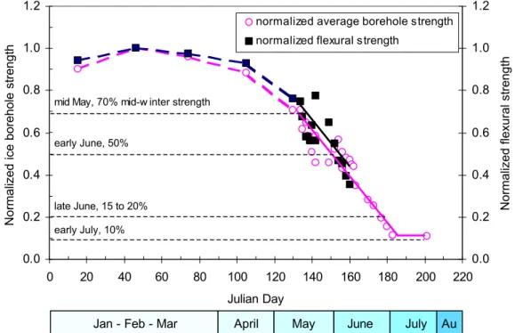
Figure 6: Comparison of ice borehole strength and calculated flexural strength The ratio of ice borehole strength to flexural strength was 43 in mid-winter and decreased to 8 in late spring. Since the relation between the two strength measurements cannot be represented by a constant ratio, the two strengths were normalized with respect to their maximum, mid-winter values. The results of the normalization are shown in Figure 7. To provide an indication of the normalized, full thickness ice borehole strength, the borehole strengths at depths 0.30 and 0.90 m (shown in Figure 5) were averaged. That averaged strength was then normalized with respect to the extrapolated, average, mid-winter strength of the two ice depths (25.5 MPa). A similar procedure was used for normalizing the flexural strength (maximum mid-winter strength of 0.71 MPa).
The trends of decreasing normalized strengths in Figure 7 are in excellent agreement with one another. Both strengths show that in May, the ice had about 70% of its mid-winter strength. By early June, the ice had about 50% of its mid-mid-winter strength. After the first week of June, only the borehole jack measurements provided information about the degradation in ice strength. Measurements showed that by the end of June, the ice had only 15 to 20% of its mid-winter strength. The ice strength was stable during the month of July, when only 10% of the mid-winter ice strength remained. [To put this in perspective, this flexural strength value for the sea ice of approximately 70 kPa is only slightly higher than the flexural strength of ice using in physical modelling facilities. In physical model tests, the flexural strength of the model ice is typically on the order of 30 to 60 kPa.]
0.0 0.2 0.4 0.6 0.8 1.0 1.2 0 20 40 60 80 100 120 140 160 180 200 220 Julian Day
Normalized ice borehole strength
0.0 0.2 0.4 0.6 0.8 1.0 1.2
Normalized flexural strength
normalized average borehole strength normalized flexural strength
April May June July Au
Jan - Feb - Mar
mid May, 70% mid-w inter strength
early June, 50%
late June, 15 to 20% early July, 10%
Figure 7: Comparison of normalized ice borehole strength and calculated flexural strength
The correlation between the ice strength and air temperature is shown in Figure 8. Increasing air temperatures are the primary reason for the decrease in ice strength during the decay season. Once the air temperature warms to about –10°C, the majority of the internal salts within the ice have converted from the solid phase to the liquid phase, and the sea ice is no longer in its mid-winter state. After the ambient air temperatures rise above about –10°C, the brine pockets rapidly begin to increase in size, causing a decrease in ice strength. Figure 8 shows that the decrease in ice strength continues until early July, by which time the ice has about 10% of its mid-winter strength.
2.9 Ice Strength and Stages of Decay
A considerable amount of work has been devoted to describing the stages of ice ablation using remotely sensed imagery. Barber et al. (1997) qualitatively described ice decay in terms of various stages of ablation. Similarly, DeAbreu et al. (2001) examined time- sequenced satellite images of landfast first-year sea ice in the Resolute region during the 2000 ice decay season. The authors described at least five stages of ablation, including sea ice in its winter state, snow melt, pond formation, pond drainage and rotten ice. Although remote sensing is an effective means of monitoring processes that occur at the ice surface, it does not provide information about the bulk layer of ice. One of the objectives of the 2000 and 2001 seasons of field measurements was to relate remotely sensed observations to changes within the internal layers of ice.
HYD-TR-070 Page 20
Since the work of DeAbreu et al. (2001) coincided with the area in which the ice borehole strength measurements were performed, DeAbreu’s five stages of ablation were superimposed in general terms on Figure 8. The snow melt stage began in mid-May and extended to late-June. Ice strength during the snow melt stage ranged from 70 to 40% of its mid-winter strength. After the snow melt stage, melt ponds began to form on the ice surface. The ponding stage occurred in late June and lasted for about one to two weeks. During the ponding stage, the ice had about 30 to 20% of its mid-winter strength. Melt pond drainage began in early July and continued throughout the month. Ice strength during the pond drainage stage was from 20 to 10% of the mid-winter ice strength. Once the melt ponds drained from the ice, it was considered rotten ice, the most advanced stage of decay. No information was available about the strength of rotten ice.
0.0 0.2 0.4 0.6 0.8 1.0 1.2 0 20 40 60 80 100 120 140 160 180 200 220 Julian Day Normalized ice s trength -50 -40 -30 -20 -10 0 10
Resolute mean daily air tempera
ture (
o C)
April May June July Aug
Jan - Feb - Mar
winter snowmelt Pond Drain Rotten
air temperature (10 pt average superimposed)
early June, 50%
late June, 15 to 20% early July, 10%
m id May, 70% mid-winter strength
3.0 MULTI-YEAR AND SECOND-YEAR ICE
3.1 Strength of Multi-year Ice
In contrast to first-year ice, multi-year ice and second-year ice have very low salinities. As such, there is little porosity in the ice and it is considerably stronger than first-year sea ice. Further, since there is little salt, there is not a large change in the brine volume with increasing temperature. There is, however, a general decrease in strength with increasing temperature, but this is mostly as a result of the decreasing strength of the ice matrix itself. In many ways, multi-year ice is similar to freshwater ice and glacial ice.
Although there have been a large number of strength tests performed on freshwater ice, only a handful of tests have been performed on multi-year and second-year ice. There have been no reported measurements of the flexural strength of multi-year ice. However, there have been a number of measurements of the compressive strength of multi-year ice (Timco and Frederking, 1982; Sinha 1984; Cox et al., 1984) and second-year ice (Sinha, 1985). These measurements showed that (1) the strength of the multi-year ice is similar to the strength of first-year ice when the ice is very cold (i.e. -20°C), but (2) multi-year ice is considerably stronger than first-year ice when the ice is warmer. This is a reflection of the lack of brine volume increase with increasing temperature with multi-year ice.
There have been very few reports of the borehole jack strength of multi-year ice published in the open literature (Iyer and Masterson, 1987; Blanchet et al., 1997). However, there were a number of field measurement programs carried out in the 1970s and 1980s as part of the oil and gas exploration in the Beaufort Sea. The results of these studies are not available publicly, but they are available to the CHC as part of the NRC Centre of Ice-Structure Interaction (Timco, 1998).
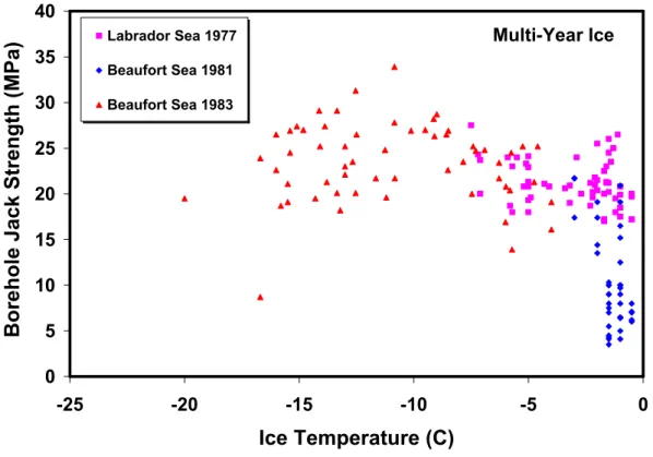
Fenco (Dome Petroleum, 1982) carried out a series of borehole jack tests in multi-year ice during August and October 1981 field trials. Geotech carried out borehole jack tests during two field programs to the Canadian Arctic. During the 1982 test program reported by Dome (1982), 40 borehole jack tests were performed. For the Geotech (1984a) study, 60 borehole jack tests were done using the conventional borehole jack, and 22 tests were done at a higher rate (fast borehole jack tests). For the latter tests, the time to the peak pressure was less than 0.5 s, which is substantially quicker than the conventional loading times, which averaged about 10 seconds. Detailed information on the Geotech (1983) field program was not available, although Geotech reported that there were 33 vertical tests performed with an average strength of 30.1 MPa, and 9 horizontal tests performed with a mean strength of 26.5 MPa. In addition to these Beaufort Sea studies, Fenco (1977) measured the borehole jack strength of multi-year ice off the coast of Labrador. The information from these field studies was extracted and plotted as a function of temperature in Figure 9.
HYD-TR-070 Page 22 Multi-Year Ice 0 5 10 15 20 25 30 35 40 -25 -20 -15 -10 -5 0 Ice Temperature (C)
Borehole Jack Strength (MPa)
Labrador Sea 1977 Beaufort Sea 1981 Beaufort Sea 1983
Figure 9: Borehole jack strength as a function of ice temperature for multi-year ice. Figure 9 shows that the strength of multi-year ice is not a strong function of temperature until very close to the melting point. Strength values for colder ice are in the range of 18 to 35 MPa. In the temperature range above -2°C, there can be a very large range of ice strength. The data indicate that the strength of very warm multi-year ice can range from 4 to 26 MPa.
It should be noted that the strength of first-year sea ice in mid-winter is of the order of 20 to 28 MPa (see Figure 5), which is not dissimilar to the strength of cold multi-year ice as shown in Figure 9. This is a reflection of the fact that most of the salt in first-year sea ice is in its solid state, and as such, there is little brine porosity in the ice. As the melt season progresses, however, the strength of first-year ice decreases considerably more than that of multi-year ice.
3.2 Decay Process in Multi-year Ice
Virtually nothing is known about the actual decay process in multi-year ice. As discussed above, there have been only a limited number of measurements on multi-year ice throughout the winter and spring seasons. The information available is not conclusive for making any concrete statements about the decay process. There are a few things to note in this regard for multi-year ice:
1. The limited number of borehole jack tests at higher temperatures do not show a strong temperature dependence, indicating that multi-year ice does not decay in the same manner as first-year ice. This is understandable based on the phase relationships of the salts and the low salinity of multi-year ice.
2. Multi-year ice can decay. Figure 9 shows a decrease in strength very close to the melting point of the ice. Further, large multi-year ice floes have broken apart very easily with the MV Arctic (B. Gorman, personal communication). It is not clear, however, whether this was due to lower ice strength or a relatively thin multi-year ice floe.
3. There is no visual method for judging if multi-year ice has decayed.
4. The large range of strength values for multi-year ice close to the melting point indicates that temperature cannot be used as a method for defining low strength for multi-year ice.
5. Freshwater ice decays through a “candling” process. This comes about from the absorption of solar radiation at the impurities at the grain boundaries of the individual ice crystals. For freshwater ice, the grain structure is often columnar, and when sufficiently decayed, the ice breaks apart in a large number of long slender columns that resemble candlesticks. This process could also play a role with multi-year ice, but it is not clear how deep this candling process would occur within the ice.
3.3 Decay of Multi-year Ice and the Ice Regime System
Based on the limited information available on the decay of multi-year ice, there is no scientifically-based reason to increase the Ice Multiplier for decay of multi-year ice. It should be noted that in the original ASPPR document (ASPPR, 1989) there is no adjustment for the decay of multi-year ice. However, in the Arctic Ice Regime Shipping System Standards (AIRSS, 1996) there is a bonus given for the decay of multi-year ice. The authors do not know the reason for this change.
Based on this analysis, the following recommendations are made for multi-year ice: 1. The bonus of +1 to the Ice Multiplier should not be given for decay of multi-year
ice. It is recommended that the approach proposed in the ASPPR be re-adopted; 2. Field measurements of multi-year ice throughout the summer season should be
undertaken to provide more insight into the decay and strength of multi-year ice. This work would provide the necessary information for making the final decision on the issue of decayed multi-year ice and the Ice Regime System.
HYD-TR-070 Page 24
4.0 SHIP DAMAGE IN THE CANADIAN ARCTIC
The current Ice Regime System gives a bonus of +1 to the Ice Multipliers if the ice is decayed. In this section, an analysis will be made to investigate whether there is any evidence to support this bonus to the Ice Multiplier.
As a first step, it is necessary to understand the volume and timing of vessel traffic in the Arctic. The majority of vessel traffic occurs during the summer months. This traffic is primarily comprised of commercial shipping for transporting goods to the Arctic, removal of natural resources from mines, fishing vessels, tour boat operations and regulatory vessels. In the 1970’s and 1980’s there also was some activity in the Beaufort Sea related to offshore oil and gas exploration. At the present time, this Beaufort activity has stopped. To quantify the volume of traffic, use was made of a database developed by Mariport Inc. They have compiled a list of vessel traffic in the Arctic for several years. For the present analysis, the data from 1996 was used. In this year, Mariport reported that there were 59 different vessels in the Canadian Arctic. These data were analysed to count the number of different vessels that were in the Arctic during each month of the 1996 calendar year. Figure 10 shows the results in a histogram with the months indicated numerically from 1 to 12 (January to December). From this figure is clear that there is some limited shipping in June and July, but the majority of traffic takes place during August and September.
0 5 10 15 20 25 30 35 40 45 1 2 3 4 5 6 7 8 9 10 11 12 Month Number of Vessels 1996 Data
Figure 10: Vessel traffic in the Canadian Arctic by month for the 1996 calendar year (data from Mariport Inc.)
The Canadian Hydraulics Centre has developed a database related to vessel damage due to ice, as part of their work to put the Ice Regime System on a scientific basis (Timco and Kubat, 2001). This database contains over 1500 Events related to both damage and no-damage Events of ships in ice-covered waters. The database was queried to extract the information related to vessel damage due to ice. The query included all types of damage (not just hull-related damage). The data was filtered to look at regions with latitude north of 57° and includes approximately 20 years of damage statistics. The vast majority of the damage Events relates to the Canadian Arctic, but there are also a few Events in the American Arctic and in the Baltic Sea. Figure 11 shows a histogram of the results. The data have been further separated based on the presence of multi-year ice at the time of the vessel damage. There are several things to note in this figure:
• The shape of the histogram is very similar to Figure 10; i.e. there are more damage events with more vessel traffic.
• The largest number of damage events occurred in August, with slightly fewer damage Events in both July and September.
• In July, there are a large number of Events in which only first-year ice is present. • Between August and October, there are a similar number of damage events with
multi-year ice present, but a decreasing number with only first-year ice present.
0 10 20 30 40 1 2 3 4 5 6 7 8 9 10 11 12 Month
Number of Damage Events
First-year Ice only Old Ice in Ice Regime
N = 130
Figure 11: Histogram showing the number of damage Events in the Arctic for each month
HYD-TR-070 Page 26
5.0 FIRST-YEAR ICE DECAY AND THE ICE REGIME SYSTEM
The current Ice Regime System takes into account the large difference in strength between mid-winter ice and summer ice by introducing the “decay” of the sea ice. This is done by allowing the addition of +1 to the Ice Multiplier when the ice is decayed to the “rotten” stage. This is a very qualitative approach. The definition of the rotten stage is not quantitatively well-defined (and it is not easily detectable). Further, as can be seen from Figure 7 and Figure 8, there is not an abrupt change in strength at any time – rather, there is a continual decrease in the strength of the ice once the air temperature begins to rise. This decrease in strength is directly related to the rise in the air temperature. The data show that the strength of the ice sheet has decreased to approximately 20% of its mid-winter strength when the mean ambient air temperature remains consistently above 0°C. Further, when the air temperature remains above 0°C for several weeks, the strength of the ice drops to approximately 10% of its mid-winter strength. This analysis provides a quantitative method for incorporating the difference in mid-winter and summer strength. Measurement of air temperature is very easy. The present analysis has shown that this property can be directly related to the strength of first-year sea ice. This can be used as a means of defining the stage at which the summer bonus could be given to the Ice Multiplier for first-year sea ice.
When should the summer bonus be given? There are several aspects that must be considered for this. The data show that the strength of the ice is approximately 20% of the mid-winter strength once the air maintains a temperature of 0°C for a few days. This is a result of a gradual increase in temperature during the spring with a resultant decrease in strength. Does this value seem reasonable to take for the summer bonus? For the Arctic, above zero temperatures occur typically at the end of June. An examination of the ship traffic and damage statistics (see Figure 10 and Figure 11) shows that there are a large number of damage incidents during July when the vessel traffic is still relatively low. Thus, a value of 20% of winter strength is too high. If a value of 10% of mid-winter strength were used, this would typically occur in early August; i.e. one month with ambient air temperatures above 0°C. This strength of the ice at that time should not present any potential hazard for ice-strengthened vessels. Further, the ice at this time has thinned considerably from its mid-winter thickness (see Figure 3).
It should be borne in mind that the Ice Regime System is related to safety, not operational efficiency. Thus, it could be argued that decayed ice allows the vessels to travel at higher speeds where there is more risk of damage with a collision with a multi-year floe. This should be considered in the application of the summer bonus.
The present analysis shows that there is a good reason to take into account the strength of sea ice in the Ice Regime System. Since the Regulations must cover all of the calendar year, they should be structured to take this large strength difference into account. This is necessary not only for the spring season, but also for the autumn season when the ice is forming and increasing in strength.
Based on this analysis, the following recommendations are made with regard to first-year sea ice decay:
1. The concept of decay of sea ice should be re-cast in terms of the strength of the ice in the Ice Regime System.
2. There should be a bonus given for low strength during the summer months, since the ice is considerably weaker and thinner than in mid-winter.
3. The springtime (i.e. melt) limit for the summer bonus could be based on the present analysis. It is noted that the strength of ice can be directly related to the ambient air temperature. This is a convenient and easily-measured quantity to define the summer bonus. It is proposed that the summer bonus be given once the ambient air temperature has been above 0°C for one month.
4. Additional analysis should be performed to define a similar criterion to be used during the autumn/winter growth season.
HYD-TR-070 Page 28
6.0 SUMMARY AND RECOMMENDATIONS
The analysis presented in this report has clearly shown that there is no quantitative scientific basis for the current approach of taking into account the decay of sea ice in the Ice Regime System. The present analysis pointed towards an approach to take into account the large difference in strength between mid-winter and summer ice. To do this, it is recommended that:
1. The concept of decay of sea ice should be re-cast in terms of the strength of the ice in the Ice Regime System.
2. There is justification to provide a bonus given for low strength during the summer months, since the ice is considerably weaker than in mid-winter.
3. The bonus of an increase of +1 to the Ice Multipliers can be based on the ambient air temperature since this is directly related to the strength of first-year ice. It is proposed that the summer bonus be given once the ambient air temperature has been above 0°C for one month.
4. A detailed analysis should be done on the strength of ice during the growth (i.e. autumn) season to define a similar criterion to be used during the growth season. 5. The bonus of +1 to the Ice Multiplier should not be given for decay of multi-year
ice. It is recommended that the approach proposed in the ASPPR be re-adopted; 6. Field measurements of multi-year ice throughout the summer season should be
undertaken to provide more insight into the decay and strength of multi-year ice. This work would provide the necessary information for making the final decision on the issue of decayed multi-year ice and the Ice Regime System.
This work should be carried out in conjunction with the Canadian Ice Service. Appropriate discussions should be held with the important Stakeholders of the Ice Regime System to ensure that the approach developed is both practical and easily implemented.
7.0 REFERENCES
AIRSS 1996. Arctic Ice Regime Shipping System (AIRSS) Standards, Transport Canada, June 1996, TP 12259E, Ottawa. Ont., Canada.
ASPPR, 1989. Proposals for the Revision of the Arctic Shipping Pollution Prevention Regulations. Transport Canada Report TP 9981, Ottawa. Ont., Canada.
Barber, D. 1997. Sea Ice Decay: Phase I. Centre for Earth Observation Science, University of Manitoba, Winnipeg, Canada, March 1997, 108 pp.
Billelo, M. 1980. Maximum Thickness and Subsequent Decay of Lake, River and Fast Sea Ice in Canada and Alaska, United States Corps of Engineers, CRREL report 80-6, February, 1980, 160 pp.
Blanchet, D., Abdelnour, R. and Comfort, G. 1997. Mechanical Properties of First-year Sea Ice at Tarsiut Island. Journal of Cold Regions Engineering, March 1997, Vol. 1, No. 1, pp. 59 – 83
Cox, G., Richter-Menge, J., Weeks, W., Mellor, M. and Boswoth, H. 1984. Mechanical Properties of Multi-year Ice, Phase 1: Test Results. US Army CRREL Report 84-9, Honover, NH, USA.
Cox, G. and Weeks, W.F. 1974. Salinity Variations in Sea Ice. J. Glaciology. Vol 13, No. 67, pp 109-120.
Cox, G. and Weeks, W. 1982. Equations for Determining the Gas and Brine Volumes in Sea Ice Samples. CRREL Report 82-30, Hanover, N.H., USA.
Cox, G. and Weeks, W. 1988. Profile Properties of Undeformed First-year Sea Ice. CRREL Report 88-13, Hanover, N.H., USA.
DeAbreu, R., Yackel, J., Barber, D., and Arkette, M, 2001. Operational Satellite Sensing of Arctic First-Year Sea Ice Melt. Can. J. of Remote Sensing, Vol. 27, No. 5, October 2001, pp. 487 – 501.
Dome Petroleum, 1982. Tarsiut Island Data Analysis 1981-1982. Dome Petroleum Report APOA 213, Calgary, Al., Canada.
Fenco, 1977. 1977 Winter Field Ice Survey Offshore Labrador. Report submitted to Total Eastcan Exploration Ltd., Calgary, AL., Canada.
Frankenstein, G.E. and Garner, R., 1967. Equations for Determining the Brine Volume of Sea Ice from -0.5 to -22.9 C. Journal of Glaciology, Vol. 6, No. 48, pp. 943-944.
HYD-TR-070 Page 30
Geotech, 1984. Multi-Year Ice Strength Test Program, Phase II. Report 9100 submitted to Gulf Canada, Calgary, Al. Canada.
Geotech, 1983. Multi-Year Ice Strength Testing Program for Gulf Canada Resources Inc. Report submitted to Gulf Canada, Calgary, Al. Canada. (APOA 200).
Iyer, S.H. and Masterson, D.M. 1987. Field Strength Tests of Multi-Year Ice using Thin-Walled Flat Jacks. Proceedings POAC’87, Vol. 3, pp 57-73, Fairbanks, AL, USA.
Johnston, M., Frederking, R. and Timco, G. 2000. Seasonal Decay of First-year Sea Ice, Technical Report by Canadian Hydraulics Centre HYD-TR-058, April 2001, 24 pp. Johnston, M. and Frederking, R. 2001. Decay Induced Changes in the Physical and Mechanical Properties of First-year Sea Ice. Proceedings Port and Ocean Engineering under Artic Conditions, POAC’01, Vol. 3, pp. 1395-1404, Ottawa, Canada.
Masterson, D.M., Graham, W.P., Jones, S.J. and Childs, G.R. 1997. A Comparison of Uniaxial and Borehole Jack Tests at Fort Providence Ice Crossing, 1995. Can. Geotech. J., Vol. 34, pp. 471 – 475.
Sinha, N.K. 1984. Uniaxial Compressive Strength of First-year and Multi-year Sea Ice. Can. J. Civil Eng., 11, pp 82-91.
Sinha, N.K. 1985. Confined Strength and Deformation of Second-Year Columnar-Grained Sea Ice in Mould Bay. Proceedings OMAE’84, Vol. 2, pp 209-291, Dallas, Tx, USA.
Timco, G.W. 1998. NRC Centre for Ice Loads on Offshore Structures. NRC Report HYD-TR-034, Ottawa, Ont., Canada.
Timco, G.W. and O’Brien, S. 1994. Flexural Strength Equation for Sea Ice. Cold Regions Science and Technology, Vol., 22, pp. 285 – 298.
Timco, G.W. and Frederking, R. 1982. Compressive Strength of Multi-year Ridge Ice. Proceedings Workshop on Sea Ice Ridging and Pile-up. NRC/DBR Technical Memo 134, Calgary, Al, Canada.
Timco, G.W. and Frederking, R.M.W. 1996. A Review of Sea Ice Density. Cold Regions Science and Technology, Vol., 24, pp. 1 – 6.
Timco, G.W. and Kubat, I. 2001. Canadian Ice Regime System: Improvements using an Interaction Approach. Proceedings POAC’01, Vol 2, pp 769-778, Ottawa, Ont., Canada.
PUBLICATION DATA FORM - FORMULE DE DONNÉES SUR LA PUBLICATION 1. Transport Canada Publication No.
No de la publication de Transports Canada
TP 13871 E
2. Project No. - No
de l’étude 3. Recipients Catalogue No.
No de catalogue du destinataire
4. Title and Subtitle - Titre et sous-titre
Ice Decay and the Ice Regime System
5. Publication Date - Date de la publication
December 2001
6. Performing Organization Document No.
No du document de l’organisme
HYD-TR-070
7. Author(s) - Auteur(s)
G.W. Timco, M. Johnston and I. Kubat
8. Transport Canada File No.
No de dossier de Transports Canada
9. Performing Organization Name and Address - Nom et adresse de l’organisme exécutant
Canadian Hydraulics Centre
National Research Council of Canada Ottawa, Ont. K1A 0R6
10. DSS File No. - No
de dossier - ASC
11. DSS or Transport Canada Contract No.
No
de contrat - ASC ou Transports Canada
12. Sponsoring Agency Name and Address - Nom et adresse de l’organisme parrain
Transport Canada Marine Safety 330 Sparks St.
Ottawa, Ont. K1A 0N8
13. Type of Publication and Period Covered Genre de publication et période visée
Technical Report
14. Sponsoring Agency Code -Code de l’roganisme parrain
15. Supplementary Notes - Remarques additionelles 16. Project Officer - Agent de projet
V.M. Santos-Pedro
17. Abstract – Résumé
The Canadian Ice Regime System takes into account the decay of sea ice by allowing the addition of +1 to the Ice Multiplier for ice that is deemed to be decayed at the “rotten” stage. This report examines this approach based on an analysis of the strength of both first-year sea ice and multi-year sea ice, and the damage statistics for Arctic vessels. The analysis shows that there is no quantitative scientific basis for the current approach of taking into account the decay of sea ice in the Ice Regime System. The report provides a detailed discussion of the analysis with recommendations that (1) the decay of sea ice should be recast in terms of the strength of ice; (2) the summer bonus for reduced ice strength should be given once the ambient air temperature has been above 0°C for one month; (3) an analysis should be performed to define a similar criterion to be used during the growth (autumn) season; and (4) there should be no bonus for decayed multi-year ice.
18. Keywords - Mots-clés
AIRSS, Ice Numerals, ASPPR, Regulations, Sea Ice Decay
19. Distribution Statement - Diffusion
20. Security Classification (of this publication) Classification de sécurité
(de cette publication) Unclassified
21. Security Classification (of this page) Classification de sécurité (de cette page)
Unclassified 22. Declassification (date) Déclassification (date) 23. No. of Pages Nombre de pages 30 24. Price-Prix