An application of a proposed airdrop planning system

(1)

An Application of a Proposed Airdrop Planning System

by

Lucas Jonathan Fortier

B.S., Aerospace Engineering, Georgia Institute of Technology, 2002

SUBMITTED TO THE DEPARTMENT OF AERONAUTICS AND ASTRONAUTICS IN PARTIAL FULFILLMENT OF THE REQUIREMENTS FOR THE DEGREE OF

MASTER OF SCIENCE

IN AERONAUTICS AND ASTRONAUTICS AT THE

MASSACHUSETTS INSTITUTE OF TECHNOLOGY JUNE 2004

The author hereby grants to MIT permission to reproduce and to distribute publicly paper and electronic copies of this thesis document in whole or in part.

Signature of Author

AERO

Department of Aeronautics and Astronautics

Certified by

Certified by

Sean George Charles Stark Draper Laboratory Technical Supervisor

Dr. Brent Appleby Lecturer Informational and Control Engineering Laboratory Massachusetts Institute of Technology Thesis Supervisor

I5r. Edward M. Greitzer H. N. Slater Professor of Aeronautics and Astronautics Chair, Committee on Graduate Studies Accepted by

MSSACHUSETTS I4TUTE

JUJL o 1 2004

LiBRAR IES

(2)

(3)

An Application of a Proposed Airdrop Planning System by

Lucas Jonathan Fortier

Submitted to the Department of Aeronautics and Astronautics on May 14, 2004, in partial fulfillment of the requirements for the

Degree of Master of Science in Aeronautics and Astronautics

ABSTRACT

The United States military has always had an increasing need for more accurate airdrops, whether the drops are being implemented for various special operations missions, or for basic humanitarian relief. Improving the delivery accuracy of airdrops will result in numerous benefits. In attempting to improve airdrop accuracy, it is helpful to know what errors will arise throughout the course of a drop. This information is effective in revealing to the airdrop personnel what steps can be taken to improve the airdrop, as well as what the expected landing accuracy of the airdrop will be. This research converges on tools to assist in the estimation and improvement of airdrop landing errors.

Wind estimation was studied to better understand the landing errors that stem from different wind prediction methods, as well as from onboard wind measurement systems. Other uncertainties, throughout each phase of an airdrop, are also known to produce landing errors, such as uncertainties in release conditions and parachute dynamics. These errors were implemented in airdrop simulations, for both unguided air release planning systems and guided airdrop systems, to determine the effects of these uncertainties on landing error.

Error in wind estimation was found to be the largest source of error in the airdrop simulations. Guided systems were hypothesized to have much smaller landing errors than the unguided systems, and that hypothesis was confirmed in this study. One major benefit of using guidance was the ability to implement onboard wind measurement systems. Using the data from the simulation results, this information was combined to produce an airdrop planning aid to assist airdrop personnel in their aerial deliveries. While the tool developed in this study is not a complete product, it represents a template on which to base further airdrop planning aids.

Technical Supervisor: Sean George

Title: Laboratory Technical Staff

Thesis Supervisor: Dr. Brent Appleby

(4)

(5)

Acknowledgments

I would like to sincerely thank the Charles Stark Draper Laboratory for providing me with the wonderful opportunity to pursue an advanced degree at MIT. I am especially grateful to my project supervisors, Dr. Brent Appleby, thesis supervisor, and Sean George, technical supervisor, for their supportive assistance in my research.

I would also like to thank Roberto Pileggi, Tom Fill, Philip Hattis, and Professor Wallace VanderVelde for their assistance with this project

This material is based upon work supported by the Army Contracting Agency -Yuma, under contracts DABJ49-03-C-00 13, W9124-04-C-0018 and DATMO-02-C-0039. Any opinions, findings and conclusions or recommendations expressed in this material are those of the author(s) and do not necessarily reflect the views of the Army Contracting Agency-Yuma.

This material is also based upon work supported by Draper Internal Research and Development. Publication of this thesis does not constitute approval by Draper or the sponsoring agency of the findings or conclusions contained herein. It is published for the exchange and stimulation of ideas.

(6)

(7)

The United States military has always had an increasing need for more accurate airdrops, whether the drops are being implemented for various special operations missions, or for basic humanitarian relief. Improving the delivery accuracy of airdrops will result in numerous benefits. A key benefit will be reduced losses of airdropped supplies by facilitating the placement of these supplies where they are needed. Accounts of airdrops from the Vietnam War, for example, describe situations where airdropped supplies to the French army missed their target and ended up with the enemy. Airdrops can also be made safer for the aircrews by allowing airdrops to be released from higher altitudes while still enabling the dropped supplies to reach the target [1]. Planes flying in enemy territory are at higher risk to anti-aircraft weapons at lower altitudes. Improving accuracy will also allow airdrops to be performed in more places than the current technologies permit, as drop zones must be large enough to account for any errors that might arise throughout the course of the drop [2]. Attempting to place airdropped payloads into too small of an area could not only result in loss or damage to the payload, but could incur damage on surrounding buildings, structures, and people.

Conventional military airdrops consist of 'round' unguided parachute systems with no ability to be steered once in the air. Figure 1.1 shows a picture of conventional canopies.

(14)

Figure 1.1. G-12s Airdropped from a C-130

Several factors are helpful in improving the accuracy of these conventional airdrops. Enhancing the determination of the optimal release point from the release conditions and the estimated wind patterns is one objective for improving accuracy. Improving the wind sensing ability is also known to be an effective technique in improving airdrop accuracy, as the better the wind conditions are known, the better the release point can be calculated. Using a guided delivery system is another means of improving airdrop accuracy by allowing the system to steer itself towards the target throughout the descent [3]. Figure 1.2 displays a parafoil that a guided system can control.

(15)

Draper Laboratory has been developing technologies to improve accuracy of both unguided and guided airdrop systems. A guided system known as PGAS, or Precision Guided Airdrop System, was developed to provide accurate delivery within 100 meters of the target [2]. The parafoil actually achieved landing accuracies of about 35 meters, with much of the landing attributed to uncertainties in GPS altitude [2]. A ballistic system known as WindPADS, or Wind-Profile Precision Aerial Delivery System, was also developed to improve the delivery accuracy of 1000-2200 pound payloads via high altitude airdrop. WindPADS combines an onboard airdrop planner with a wind and density field estimator to enable more accurate airdrops [1]. Draper followed this with the development of a guided airdrop planning system, which combined the guidance ability from PGAS with the airdrop planning ability from WindPADS.

This project attempts to continue the pursuit of improving airdrop accuracy. The driving sources of error are identified for various airdrop situations. These driving sources of error should be given more importance when seeking methods to reduce landing errors. Using the error analysis, a tool is developed to assist in the planning phase of an airdrop. This planning tool is able to predict the landing accuracy that can be attained for a given system. The tool is also able to determine what types of adjustments can be made to the airdrop situation to achieve a desired accuracy. The tool developed in this study is not a generic product, as it is only representative of the systems used in this study. However, the methodology behind the planning tool represents a template for developing a practical airdrop planning aid for a wide range of airdrop systems.

1.2 Simulation Overviews

In this study, two separate simulations were utilized to simulate actual airdrops. For unguided airdrop analysis, a simulation from the WindPADS program was used known as PADS, or Precision Aerial Delivery System. The PADS simulation handles three degree-of-freedom dynamics models, along with experimental look-up tables, of unguided, ballistic airdrop systems. All phases of airdrop flight are analyzed, including:

(16)

extraction, stabilization, steady-state descent, and landing. PADS can handle a variety of different aircraft, parachutes, and payloads, among other variable parameters. Also included in the software is the capability for Monte Carlo simulation, which is useful in probabilistic error analysis.

For guided airdrop analysis, the simulation from the PGAS program was used. The simulation utilizes representations of parachute dynamics, navigation sensors, expected environment, and onboard wind measurement systems. The type of parafoil used in this simulation is known as the "Wedge 3," which was developed by the NASA Dryden Flight Research Center (DFRC). The parafoil has a surface area of 88 square feet [2]. Although PGAS has the ability to handle various types and sizes of parafoils, only one kind will be used to analyze the performance of guided airdrop systems. Like the PADS simulation, the PGAS software is capable of performing Monte Carlo simulations.

1.3 Thesis Outline

The primary goal of this thesis is to develop a tool to assist in the planning phase of an airdrop. Wind conditions and wind knowledge have been known to be a major factor in the accuracy of airdrops; therefore wind prediction errors are analyzed and modeled, along with methods for developing realistic wind conditions. Both unguided and guided systems are simulated to determine the driving errors for each respective system. Total expected landing errors for these systems are also determined. These findings are then brought together to develop the tool to assist in airdrop planning.

Chapter Two describes several wind prediction methods that are used throughout this study. The errors that these wind prediction methods provide are determined and modeled. Techniques for generating realistic wind conditions are discussed, along with algorithms to effectively integrate onboard wind measurement systems into the airdrop system's wind prediction.

(17)

Chapter Three analyzes the errors present in unguided air release planning systems. Individual error sources, including errors in release conditions, parachute dynamics, and wind conditions, are examined to determine the driving error sources inherent in the system. Expected landing errors are determined for various scenarios, and methods for error reduction are discussed.

Chapter Four analyzes the errors present in guided airdrop systems. Similar to the study of unguided systems in Chapter Three, expected landing errors are determined for various scenarios. Different methods of pre-drop wind knowledge are examined, as well as methods of achieving wind knowledge during the descent.

Chapter Five combines the results from Chapters Three and Four and develops a tool to assist in the planning phase of the airdrop. This tool does not represent a generic product that can be currently used for any airdrop system, but rather a template to develop a practical airdrop planning aid. Examples of the use of this planning tool are shown to display its ability to determine what kind of accuracy is attainable with a given system, and to determine what types of adjustments can be made to the airdrop situation to achieve a desired accuracy.

Chapter Six presents the conclusions of this research effort and makes recommendations for further study in the area of airdrop accuracy.

(18)

(19)

Chapter 2 Wind Characteristics

2.1 Introduction

Airdrop systems are never completely accurate. There are many factors that affect the landing location of an airdrop, chief among them being the wind conditions at the time of the drop. It is important to understand the behavior and uncertainty statistics of wind when making wind predictions, as wind prediction error can be one of the most significant sources of landing error. This chapter is devoted to modeling wind prediction errors to assess the impact that wind error has on airdrop accuracy.

Methods for developing wind predictions are discussed below. Along with the different wind prediction methods, there are different techniques for describing the wind prediction errors to assess the impact that wind has on airdrop accuracy. Some of these methods are also discussed below, and one method is chosen to be the technique to be used throughout the remainder of this study.

The wind samples used in this study for purposes of wind modeling and wind error prediction are taken from Yuma, Arizona. This is mainly because a large sampling of wind from Yuma was readily available. Therefore, most of the succeeding wind data will be specific to Yuma; however, the statistical methods used here, as well as the general insights gained from this research can be applied to wind analysis anywhere.

(20)

2.2 Wind Prediction Methods

There are numerous methods to develop wind predictions. The most basic method, and least accurate, is to use general wind statistics for the area where the airdrops are to be performed. This historical data is usually in the form of monthly or daily averages of wind speeds at various altitudes.

Weather forecasting is a more accurate predictor of wind than the general wind statistics. Forecasts can be made at any time preceding an airdrop, with the more accurate forecasts using wind data closer to the drop. There are many methods to enhance forecasts, including the use of balloons and/or dropsondes to provide updated wind samples for the forecast.

The most accurate wind prediction method is onboard sampling. This is only effective for guided airdrop systems, as only the guided system can alter its course depending on the updated wind knowledge after it is dropped. One type of onboard sampling is to measure the wind at the current altitude, and estimate the winds at lower altitudes using the current measurement. Another type of onboard sampling is to measure the winds at lower altitudes and use that measurement to estimate the winds at other altitudes. This can be done with a LIDAR system, among others, and is a powerful method for measuring the wind field that the system will encounter.

2.2.1 General Wind Statistics

There has been a joint effort between the United States Navy and the Department of Commerce to produce general wind statistics for various locations around the world. One of those locations is Yuma, Arizona. For eight years (1980-1987), wind measurements were taken twice daily at various altitudes by use of radiosonde launches, aircrafts, and satellites. Although differences were noticed between winds during different months, these differences were small. It was therefore acceptable to generalize the wind patterns

(21)

over the entire year, rather than month-to-month. Table 2.1, shown here, displays the general wind statistics for Yuma, Arizona at given altitudes.

Table 2.1. General Wind Statistics for Yuma, Arizona

Average (ft/s) Standard Deviation (ft/s) Altitude (ft) North East North East

5,000 1.4 6.9 9.0 7.0 10,000 1.1 11.7 18.8 19.3 19,000 -0.7 28.1 30.0 30.4

25,000 -0.8 38.6 36.8 37.0

It can be seen in Table 2.1 that the average North winds are much smaller than the average East winds. The average North winds are around zero ft/s. The East winds, however, have a non-zero average that increases with altitude. Using a least-squares method for a linear curve-fit, one can derive a function for the averages and standard deviations of North and East winds as a function of altitude. The linear approximations (in the form y = mx + b) are shown below in Table 2.2.

Table 2.2. General Wind Statistics Approximation Parameters

Parameter North Mean North St. Dev. East Mean East St. Dev.

Slope (s-') -0.0001 0.0014 0.0016 0.0014

Intercept (ft/s) 2.09 3.58 -2.71 2.07

These approximations will be used later when analyzing airdrop systems under specific wind conditions.

(22)

2.2.2 Wind Forecasting Statistics

Unlike the general wind statistics, the forecasted wind files are all available in raw data form. In other words, the entire forecasted wind profiles, along with the entire corresponding measured wind profiles are available. All the wind files used in this forecasting analysis are taken from tests that the NWV team has performed, and the wind prediction method of choice was a forecast combining Air Force Weather Agency (AFWA) data along with wind measurements made by balloons. This data is the only data readily available to the NWV team for analyzing wind prediction methods and developing wind error statistics. If data from other wind prediction methods are available, similar approaches as shown in this chapter can be used to develop alternative wind error statistics that are more appropriate to the desired wind prediction method.

When the NWV team tests their unguided air release planning system, wind readings are recorded for each drop. About 15-30 minutes before each drop, a balloon is sent up to measure the wind velocity at numerous altitudes using GPS. Then, a meteorological expert working with the NWV team combines the balloon data with a weather forecast to project the winds at a later time. Three-dimensional wind fields are provided by the AFWA. This information is then assimilated with the balloon data to forecast the winds in the future. This projection is known as the predicted wind. It is with this wind prediction that the NWV team calculates the aerial release point for the payload.

When the airplane reaches the release point, the parachute is deployed out of the back of the plane. A radar apparatus on the payload of the parachute tracks its motion through its descent. The NWV team then takes that radar data and extracts what is called a truth wind. This is the actual wind that the parachute experienced during the drop.

Almost immediately after the parachute is released out of the plane, a second chute, known as a windpack, is released. The windpack is a wind measurement device that also provides a truth wind as it descends towards the ground by using a GPS receiver to record its ground track. It provides similar data to the radar wind track, with small differences

(23)

due to the different trajectory and time lapse. In comparing the predicted and the truth winds, files were provided by the NWV team. Twelve balloon predictions along with the corresponding windpack truth files, and twenty balloon predictions along with the corresponding radar truth files, provide a total of 32 prediction and truth comparisons.

2.3 Error Description Methods

2.3.1 Errors in the North and East Directions

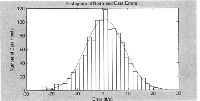
In order to determine the most appropriate system for describing the statistics of wind, it is first necessary to analyze past data. The first method considered for describing the wind prediction errors is to compare the wind velocity magnitudes in the North and East directions between the predicted and the truth winds. These are the directions used in the source files. Since North and East are arbitrary directions, their statistics can be combined to compute the statistical parameters. Errors were computed at specific altitudes, for all compatible predicted and truth files. A histogram of the errors is shown below in Figure 2.1. This histogram shows that the North and East wind errors appear to take on a Gaussian distribution with approximately zero mean.

(24)

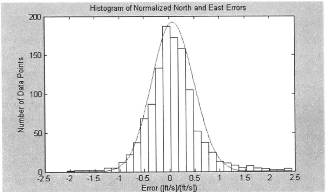
Another approach to the North and East error analysis is to normalize the wind velocity errors by the predicted wind magnitude to give a fractional error value. Normalization takes into account the magnitude of the predicted wind when describing the statistics. As in the previous figure, errors were computed at specific altitudes for all compatible predicted and truth files. A histogram of the normalized errors is shown below in Figure 2.2.

Figure 2.2. Histogram of Normalized North and East Errors

Figure 2.2 reveals that the normalized errors are also Gaussian distributed. The statistics for the original and normalized errors are shown below in Table 2.3. Extreme data points were discarded before the subsequent values were calculated to reduce any abnormal skewing that might result from extreme values. The resulting values produce close-fits to the given data. As expected, the means are close to zero.

(25)

Table 2.3. Statistical Parameters for East and North Errors

Original Errors Normalized Errors

Mean 0.84 ft/s 0.072

Standard Deviation 7.15 ft/s 0.52

2.3.2 Errors in Magnitude and Azimuth

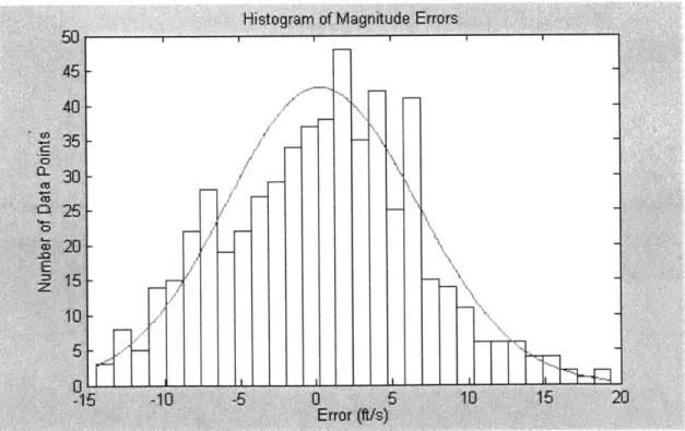
The second method of describing the errors is to compare the absolute magnitude and the azimuth angle for the predicted and the truth winds. As with the North and East errors, histograms were developed to illustrate the distributions. Figure 2.3, shown below, displays that the magnitude errors appear to take on a Gaussian distribution.

(26)

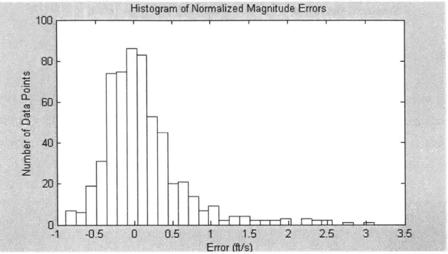
The magnitude differences were normalized with respect to the predicted wind magnitude and the histogram is shown below in Figure 2.4. This distribution also appears Gaussian, but it is improper to describe the normalized magnitude differences as Gaussian due to the fact that it is impossible to have a value less than -1.

Figure 2.4. Histogram of Normalized Magnitude Errors

The azimuth angle is the angle with respect to due north, with positive angles increasing in the clockwise direction. Similar to the magnitude errors, the azimuth errors also appear Gaussian. Figure 2.5, shown below, displays the azimuth errors histogram.

(27)

Figure 2.5. Histogram of Azimuth Errors

The statistics for the magnitude (original and normalized) and azimuth errors are shown below in Table 2.4. Extreme data points were discarded and the resulting values produce close-fits to the given data. Again, they are all approximately zero mean. Due to the fact that there is no upper bound on the magnitude error, while there is a lower bound, the mean is slightly greater than zero.

Table 2.4. Statistical Parameters for Magnitude and Azimuth Errors

Original Normalized Azimuth Errors

Magnitude Errors Magnitude Errors

Mean 0.78 ft/s 0.12 -0.17 deg

(28)

2.3.3 Error Vector Approach

The third and final method for describing errors between the predicted and the truth wind files is to calculate the error vector. The error vector is found from subtracting the predicted wind vector from the truth wind vector. In visual reasoning, it is the vector beginning at the end of the predicted wind vector, and ending at the end of the truth wind vector, as shown here.

Error Vector

Predicted Truth

Figure 2.6. Error Vector Drawing

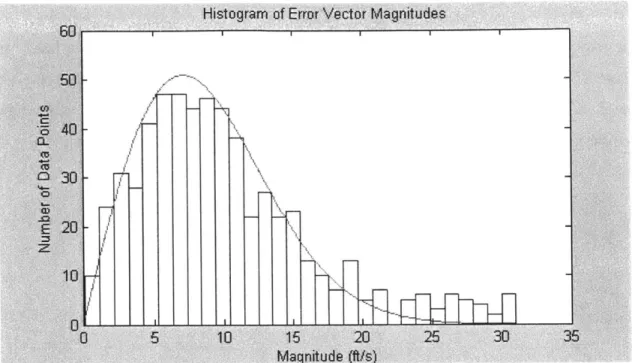
The error vector magnitude can never take a value below zero; therefore it isn't completely accurate to describe the magnitude data as Gaussian. Figure 2.7, shown below, shows the histogram of the error vector magnitudes. Although the data is not Gaussian, it still resembles an exponential function. More specifically, it bears a resemblance to a Rayleigh density function. A Rayleigh density function transpires when two orthogonal, zero mean, Gaussian components (in this case, North and East) are merged to form a magnitude and direction. The magnitude is then Rayleigh distributed.

(29)

Figure 2.7. Histogram of Error Vector Magnitudes

The error vector magnitudes were also normalized with their respective predicted wind magnitudes. Figure 2.8, shown below, displays the normalized magnitudes in a histogram. This shows an even greater resemblance to a Rayleigh distribution.

(30)

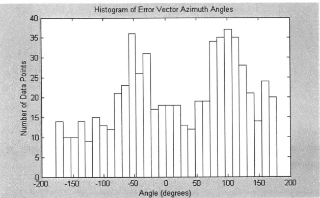
The error vector azimuth angles were computed and their histogram is shown below in Figure 2.9. There is no apparent pattern to the distribution, so it is inferred that the error vector azimuth angles are uniformly distributed. This is expected, as the angle distribution that complements a Rayleigh distributed random variable is uniform.

Figure 2.9. Histogram of Error Vector Azimuth Angles

The statistics for the error vector magnitudes (original and normalized) are shown below in Table 2.5. Again, extreme values were discarded, and the results were found to be a close fit to the given data. The only parameter needed to describe a Rayleigh distribution is the mode (or peak value). One property of a Rayleigh distribution is that the mode is equal to the standard deviation of the orthogonal components with which it was derived from. The standard deviations in Table 2.3 are approximately equal to the modes in Table 2.5, thus adhering to this property of a Rayleigh distribution. They are not exactly equal, but that is just due to the fact that different extreme values were discarded from each data set before the calculations were performed.

(31)

Table 2.5. Statistical Parameters for Error Vector Magnitudes

Original Magnitude Normalized Magnitude

Mode 8.4 ft/s 0.56

2.3.4 General Error Magnitudes

Three methods have been shown for describing the error between the predicted winds and the truth winds. These descriptions are completely independent of altitude. The only parameter that affects any of the error descriptions is the magnitude of the predicted wind. Analysis was performed to determine the effect of altitude on the statistical parameters of the errors. The results were inconclusive with the data available. Perhaps with more data, a pattern or trend in the error statistics can be observed as altitude increases or decreases. For now, the errors will be described without taking into account for altitude. In other words, the wind error standard deviation profiles will be assumed constant with respect to altitude.

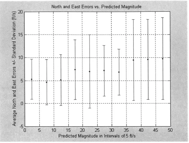
For errors in the North and East directions, as well as the error vector approach, there is still the option of using normalized errors or non-normalized errors. Figure 2.10, shown below, displays the magnitudes of the north and east errors (absolute values of the errors) given a predicted wind magnitude. The data is grouped by the predicted wind magnitudes in intervals of 5 ft/s.

(32)

Figure 2.10. North and East Errors vs. Predicted Magnitude

From the graph in Figure 2.10, it can be seen that the average magnitude of the North and East errors slightly increases as the predicted wind magnitude increases. It also appears that the range of errors (characterized by the standard deviation) also tends to grow as the predicted magnitude grows. In spite of this, the data does not show increases that are significant enough to justify the use of normalized wind errors. In the first interval, where the predicted magnitudes are between zero and five ft/s, the average North and East error magnitude is more than 100% of the predicted magnitudes. In larger ranges, such as the 35-40 ft/s range, the average North and East error magnitude is closer to 25% of the predicted magnitudes.

Because of the inconsistency across the range of predicted magnitudes, it is not accurate to describe the North and East wind errors by use of a generic normalization distribution. If normalization of the errors were desired, it would be necessary to describe the

(33)

normalization distribution as a function of predicted magnitude. In Figure 2.10, it can be shown that a vertical range from approximately 2-9 ft/s can be placed across all the error bars. This range is sufficient enough to justify the use of using a generic non-normalized distribution to describe the errors across the entire range of predicted magnitudes.

2.4 Altitude Correlation

Once the general random statistics of individual wind errors are known, the next step is to determine the correlation with respect to altitude difference for the wind errors. For a given set of n data points, X, and a corresponding set of n data points, Y, the correlation between the two data sets is given by the following formula.

n- xi. - xi -, y,

p = 2 (2.1)

n. xi- i)x, _-_n- _-_{_} y(

i

}i

li

This correlation equation was used to calculate the correlations of the wind errors with respect to the errors' altitude difference. Figures 2.11-2.14 show the correlation between the wind errors with respect to altitude difference. Figure 2.11 displays the correlations for the North and East errors. Figure 2.12 displays the correlations for the normalized North and East errors. Figure 2.13 displays the correlations for wind magnitude and azimuth errors. Figure 2.14 displays the correlations for the error vector magnitude and azimuth angles.

(34)

Correlations for North and East Wind Magnitude Errors

--- N/E Errors

+- Fitted

0 500 1000 1500 2000 2500 3000 3500 4000 4500 5000 Altitude Difference (ft)

Figure 2.11. Correlations for North and East Wind Magnitude Errors

Correlations for Normalized North and East Wind Magnitude Errors

--- data

- N- fitted

500 1000 1500 2000 Altitude Difference (ft)

2500 3000 3500

Figure 2.12. Correlations for Normalized North and East Wind Magnitude Errors 0.8 C 0 0U 0 0 U. 0.6 0.4 0.2 0 11 0.8 0.6 0.4 0.2

(35)

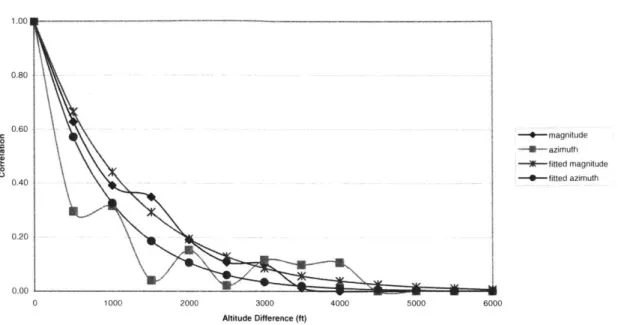
Correlations for Wind Magnitude and Azimuth Errors --- magnitude - azimuth ?I-fitted magnitude - -fitted azimuth 0.20 0.00 0 1000 2000 3000 4000 5000 6000 Altitude Difference (ft)

Figure 2.13. Correlations for Wind Magnitude and Azimuth Errors

Correlations for Error Vector Magnitudes and Azimuth Angles

1 F

500 1000 1500 2000 2500 3

Altitude Difference (ft)

000 3500 4000

Figure 2.14. Correlations for Error Vector Magnitudes and Azimuth Angles

1.00: 0.80 0.60 0.40 0 C.) 0.8 0.6 0.4 0.2 0 C.) - - 0-4500 5000 - magnitude - azimuth fitted 0 0

(36)

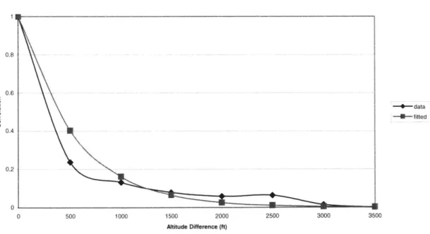
For each correlation plot, there is a generated exponential curve that fits the data. In the Global Reference Atmospheric Model (GRAM) initially developed by NASA in 1974, wind error correlations are assumed to be exponential of the form:

p = exp(-Ah / E) (2.2)

where Ah is the altitude difference and E, the correlation factor, is an empirical value that fits each specific type of data [4]. The values for c that are used in Figures 2.11-2.14 to fit the correlation data are shown below in Table 2.6.

Table 2.6. Correlation Curve-Fitting Parameters

E (ft) Figure 2.11 900 Figure 2.12 550 Figure 2.13 magnitude 1220 Figure 2.13 azimuth 890 Figure 2.14 1000

As with the uncorrelated error statistics, the correlation formulas do not depend on altitude. The correlation formulas only depend on the difference in altitude between the two points in question. This is not consistent with the GRAM model used by NASA. In GRAM, the empirical value, e, is a function of altitude. The available data was analyzed to reveal how the correlation due to the difference in altitude changes with altitude. No conclusive findings were discovered. There did not appear to be any pattern or trend for any correlation values as the altitude range was changed. Therefore, in the analysis shown here, E is a constant value throughout the range of altitudes. With more data, however, this result could be found to be inaccurate.

(37)

2.5 Generating Truth Wind Profiles

An important consequence to developing the statistics for the wind errors is the ability to generate simulated truth wind profiles based on predicted wind profiles for Monte Carlo performance analysis. The new truth wind profiles are developed from both the statistics for the individual predicted wind vectors, as well as the correlation between each predicted wind vector.

Three methods of describing winds errors were discussed; therefore it is left to the engineer which method they prefer when using the statistics to generate truth wind profiles. Method 1, errors in the North and East directions, is the simplest method due to the fact that the errors are zero mean and Gaussian. Since Method 1 is the simplest of the three methods, that will be the method implemented in the simulations throughout the project.

Method 2, errors in magnitude and azimuth, appears to be a straightforward method for generating truth winds. However, if the magnitude errors are classified as Gaussian, there is a chance that negative magnitudes will appear in the results, and a negative magnitude does not exist. That is why the normalized magnitude error can never be less than -1 (see Figure 2.4). Therefore, it is necessary to put a limit on the maximum negative error, and this causes difficulty when mathematically describing the statistics in order to generate truth winds.

Method 3, the error vector approach, is derived from Method 1. The magnitudes and azimuth angles for the error vectors are functions of the North and East errors, therefore the same results as Method 1 would be expected when generating truth wind profiles. Due to the fact that the error vector magnitudes are Rayleigh distributed makes the problem of generating correlated truth wind profiles much more difficult. Methods involving Inverse Discrete Fourier Transforms have been developed to solve this problem [5].

(38)

2.5.1 North and East Error Method of Truth Wind Generation

The North and East error method of truth wind generation for simulations was chosen due to the fact that the math involved is much simpler than the other methods. The North and East errors are assumed to be independent of each other, thus they can be handled separately. These errors are zero-mean and Gaussian distributed; therefore, it is helpful to develop a covariance matrix to generate sample error profiles. The following steps outline the means of calculating correlated sample wind errors.

All bold characters represent vectors or matrices. E [.] is the expected value of the bracketed expression.

The truth wind is equal to the predicted wind plus the error, or w = w0 + Sw.

The covariance matrix is equal to the expected value of the square of the error matrix, or C = E [6w-6wT].

Step 1. Build the covariance matrix C, where Cj = pij-i-j

pij is the correlation between the errors at two altitudes (see Equation 2.2). a is the standard deviation for each component (see Table 2.3).

Step 2. Let 6w = S-v, where v is a vector of Gaussian random variables with zero mean

and unity variance, so E [v-vT] =

Step 3. Now C = E [6w-w ] = E [S-vv.ST] = S ST.

Step 4. Given C, solve for S from C = S-ST

Step 5. Generate the error vector from Sw = S-v.

(39)

Follow Steps 1-6 for both the North wind vectors and the East wind vectors.

2.5.2 Wind Profile Generation

It is also possible to generate wind profiles without any specific measurement data available. In order to generate the profile, the general wind statistics have to be known. The winds in the North and East direction were found to be zero mean and Gaussian from the balloon and radar data. Figure 2.15, shown below, displays the standard deviation of the winds as a function of altitude.

North and East Wind Magnitude Standard Deviations

25 20 V 1 ri -+- data -- fitted 0 1000 2000 3000 4000 5000 6000 7000 8000 Altitude (ft)

Figure 2.15. North and East Wind Magnitude Standard Deviations

Although the data in Figure 2.15 shows some non-linear behavior, there is a slight upward trend, implying that wind speeds increase with altitude. The fitted line shown has a slope of 1/950 s-' and a y-intercept of 10.5 ft/s. Standard deviation is not enough to characterize the wind profile; the correlations between the winds at different altitudes are also required. Figure 16, shown below, displays the correlations between the wind velocities as a function of altitude difference.

(40)

Correlations for Wind Magnitude in One Specific Direction

data fitted

1000 2000 3000 4000 5000 6000 7000 8000

Altitude Difference (ft)

Figure 2.16. Correlations for Wind Magnitude in One Specific Direction

Unlike the correlations for errors at different altitudes, the correlations for the wind velocities are not exponential. The correlation curve in Figure 2.16 appears to follow a linear relation with respect to altitude difference, with a slope of 1/9000 ft-1.

In order to generate a random profile with the given standard deviations and correlations, the same procedure is followed as in the North and East error method of truth wind generation. The only difference is that in this case, w, is equal to zero.

The concepts of generating both predicted and truth winds are shown graphically in Figure 2.17. A random predicted wind was generated and plotted, along with the 3-sigma upper and lower limits for the wind error. Fifty truth winds were then generated and plotted on the graph. It can be seen that the fifty different truth wind profiles fall inside the 3-sigma error limits.

0.9 0.8 0.7 0.6 0.5 0.4 0.3 0.2 0.1 r-0

(41)

Figure 2.17. Predicted and Truth Wind Generation

2.6 Onboard Sampling

Guided airdrop systems can make use of insitu wind sampling as a way to decrease the errors that arise from a priori wind predictions. Onboard sampling can be used to update wind predictions from both general wind statistics and forecasting methods. An updated wind error profile is generated at each measurement and the guided parafoil will alter its position depending on the new wind error profile. The following steps outline the means

of calculating correlated sample wind errors using the onboard sampling method.

All bold characters represent vectors or matrices. E [-] is the expected value of the bracketed expression.

(42)

The truth wind is equal to the predicted wind plus the error, or w = w0 + 6w.

Step 1. Measure the wind at the current altitude. Compare the measurement with the original prediction at that altitude to get the current wind error: 6wi.

Step 2. The errors for the subsequent altitudes will be derived from the error at the current altitude with the formula: 6wi+I = aii+I- 8wi + ei+1 , where

ei+1 is a Gaussian random variable with zero mean and variance aei+sI.

Step 3. aii+1 can be found from the covariance (p) between the errors at altitudes i and i+1 and the variance of the error at altitude i as follows.

ii,i+1 = E[6wi+, Sdwi] = E[(ai.i+ 6wi + e1+1)- 6w]] = ai,+1 -E[wi2] = ij+I - ai

Step 4. ei+I2 can be found from the variances of the errors at altitudes i and i+l, along

with aiji+1 as follows.

i+ 2= E[Swiil2] = E[(ai,i+i -6wi+ ei+1)2] = aii1+2-E[6wi2] + E[ei+=2 aiji+1 ai~ + aei+

-2 2 2. 2

Therefore ei+] = ai+12 - ii

Step 5. Generate Swi+1 from Swi+i = aiii Swi + ei+1 where ei+1 is randomly generated.

Step 6. Repeat Steps 2-6 for all desired altitudes to the ground altitude.

A more detailed explanation of this algorithm is provided in Chapter 4. This method of producing wind errors is fairly accurate because it involves a known error. However, the more recursions there are down towards the ground, the more error there will be due to the repeated random number generation. This method also only takes into account the correlation of the wind error between two successive altitudes, whereas the North and

(43)

East error method of truth wind generation (section 2.5.1) accounts for the correlations between all the errors.

If onboard sampling is being used for looking ahead to the winds at lower altitudes, the same procedure for generating correlated sample wind errors is used. The only difference is the known wind error is at whatever altitude the measurements are coming from, rather than the altitude that the airdrop device is currently at.

2.7 Limitations of Results

As with many error analyses, there are limitations to the credibility of the findings and this study is no exception. First of all, the general wind statistics and the balloon prediction wind data files used in this study are specific to the Yuma Proving Grounds in Yuma, AZ. Therefore, the results shown here may not be representative of other locations with different terrains and weather patterns. Another limitation of the results shown here is the fact that there was limited data to work with. Although the 32 predicted and truth files provided lots of data points, more data is always helpful in determining statistical parameters.

There are other methods available for wind predicting, and those methods were not studied. The data used here was for two types of wind prediction methods, general statistics and balloon prediction, and was the only readily available data. The balloon prediction method used here is only good for a couple hours after the measurement update is performed (e.g., balloon data). The numerical prediction models used here, using finite-difference methods to integrate the equations of motion, are believed to be one of the best prediction methods available. However, this type of prediction method is not always readily available, and other prediction methods not studied here will provide

alternate statistical parameters.

Another imperfection of this analysis is that the measurements and predictions do not cover the exact same three-dimensional coordinates. The balloon is released at a certain

(44)

location, and travels upward into the sky collecting data to make the prediction. The parachute and/or windpack that record the truth winds do not fall in the exact path as the balloon ascension. However, due to the close proximity (usually within a mile or two),

the truth winds are considered worthy enough to be compared to the predicted winds.

Finally, no vertical components of wind were taken into account in this study. Vertical winds can have a noticeable effect on the airdrop accuracy as they alter the sinkrate throughout the flight path. The main reason this effect was disregarded is that there was not available data for vertical winds.

2.8 Conclusions

When analyzing the effects of wind prediction errors on airdrop accuracy, this study will utilize both the wind prediction methods of general statistics, as well as assimilating the AFWA prediction with the balloon measurements. Unfortunately, this was the only reliable data available for wind prediction methods. However, balloon prediction is a good representation of forecasted wind prediction. This method is the most typical and most widely used technique, and therefore the results will be more meaningful than methods that aren't used as often. The forecasting method is considered the midpoint of quality when comparing the wind prediction methods, with general statistics being the lowest quality and onboard sampling being the highest. Therefore, this method can be regarded as an average wind prediction technique.

For the balloon prediction method, the average wind error in the North and East directions was found to be approximately 7 ft/s, with little relation to altitude. The correlation factor for this type of wind error was found to be approximately 900. If other methods were available, the same procedure for analysis can be implemented, and the corresponding wind statistics can be used in airdrop accuracy studies.

(45)

Both the general wind statistics and the AFWA/balloon wind prediction methods will be used when analyzing the performance of both unguided and guided airdrop systems. Guided airdrop systems will also be analyzed with onboard sampling methods.

(46)

(47)

Chapter 3 Unguided Air Release Planning System Error Analysis

3.1 Introduction

When comparing the benefits of various airdrop systems, it is important to know what causes some systems to perform better than others. In other words, it is important to know what the sources of airdrop errors are, and to what extent these errors contribute to the landing location error. Different classes of airdrop systems have different dominant errors, and it is beneficial to know the driving errors for these systems. Consequently, the benefits of more complex systems and the requirements for particular airdrop missions

can then be evaluated.

The next two chapters are allocated to two different types of airdrop systems: unguided air release planning systems, and guided airdrop systems. This chapter is focused on determining the driving error sources for the first of these two types of systems, unguided air release planning systems. Total expected landing location errors and error sensitivities will also be examined.

3.2 Simulation Software

For error analysis with unguided air release planning systems, a simulation was used that was developed by a team at Draper Laboratory working with the Army Natick Soldier

(48)

Center under the New World Vistas (NWV) program. The simulation used for this study was PADS, or Precision Aerial Delivery System. More specifically, a version of PADS, known as PAPS (Precision Airdrop Planning System) was utilized. This simulation is a result of an effort with Draper Lab, the Army Natick Soldier Center, and several Air Force organizations to improve airdrop delivery accuracy.

The PADS simulation handles three degree-of-freedom dynamics models, along with experimental look-up tables, of unguided, ballistic airdrop systems. All phases of airdrop flight are analyzed, including: extraction, stabilization, steady-state descent, and landing. PADS can handle a variety of different aircrafts, parachutes, and payloads, among other variable parameters. Also included in the software is the capability for Monte Carlo simulation, which is useful in error analysis.

The initial simulation inputs for this study were taken from an actual airdrop performed by the NWV team at the Yuma Proving Grounds in Yuma, Arizona. The data is taken from one of a series of test drops on November 18, 2002. Many of the initial conditions for this airdrop were arbitrarily chosen as the initial conditions for all the simulation runs. Some of these conditions include: parachute type (26 foot ring-slot chute), North-East release position, release velocity, and aircraft type (C-130). Different parachutes and aircrafts could change some of the results, but the general trends of the errors are expected to be the same.

3.3 Airdrop Scenarios

In order to determine the driving errors of the airdrops, it is helpful to understand the types of conditions under which the drops are being done. For this study, a set of drop scenarios were established that would replicate typical drop conditions. These scenarios were based on four criteria: wind prediction methods, wind conditions, release altitudes, and payload weights.

(49)

For unguided systems, two types of wind prediction methods will be implemented: general wind statistics and balloon-driven forecasting. These wind prediction methods were discussed in the previous chapter.

Three different wind condition classifications were selected: light, medium, and heavy winds. Wind intensity levels are used in this study to examine the effects of overall wind intensity on airdrop accuracy. Determining what constitutes light, medium, and heavy winds is very subjective. The methods used in this study are just one of the seemingly infinite ways to describe the relative wind intensity.

The truth wind profiles that were used in the wind analysis in the previous chapter (from radar and windpack measurements) were taken, and all the North and East wind magnitudes were sorted in ascending order. These were then divided into three groups: the lower third was to represent light winds, the middle third for medium winds, and the upper third for heavy winds. The winds were to be modeled by a Gaussian distribution with zero mean and a standard deviation of sigma. The largest value in each division was defined as the three-sigma value for its particular classification of wind at the ground level altitude. The fact that we set this sigma value to the ground level is because wind magnitude was shown to increase with altitude in the previous chapter, and thus the sigma value will increase with altitude when developing wind profiles. This led to the following definitions:

Table 3.1. Wind Condition Definitions

Wind Sigma

Condition (Ground Level)

Light 3.5 ft/s

Medium 7.5 ft/s

(50)

These sigma values are used to produce wind profiles by the methods shown in the previous chapter. For the scenarios that use general wind statistics as the wind prediction method, different wind conditions are not used since the intensity of the wind is not recognized in any way.

Release altitude represents another facet of the airdrop scenario. Rather than studying many release altitude scenarios, two common altitudes were chosen: 10,000 ft and 25,000 ft. These two altitudes represent a mid-altitude test case and a high altitude test case that pushes the boundary of current operations. The final facet of the airdrop scenario is the payload weight. Three common payload weights were chosen for this study: 500, 1,000, and 2,000 pounds. These payload weights span the viable loading capabilities of the parachute being studied.

Combining these four components of the airdrop scenario, there are a total of 24 different combinations for scenarios to test the range of current operational missions. All 24 of these scenarios are simulated to determine what the driving errors are for unguided air release planning systems.

3.4 Typical Error Values

Seven parameters were recognized as major sources of error for unguided airdrops: exit time, release altitude, release course (also known as 'release heading'), release position, release speed, sinkrate, and wind. From data taken from past airdrops using the C-130 aircraft, the NWV team was able to derive typical error distributions for six of these parameters. The final error distribution, wind speed error, was derived in the previous chapter. Six of these parameters were found to have a Gaussian distribution. The non-Gaussian parameter, sinkrate error, was determined to be uniformly distributed. Their values are shown below in Table 3.2. Note that the North/East wind speed error is only

(51)

Table 3.2. Typical C-130 Error Values

There are other parameters that could affect the accuracy of an airdrop as well. However, they are considered less important. This includes factors such as parachute uniformity and the dynamic model parameters of the parachute. This could affect many parameters, including but not limited to: drag coefficients, damping coefficients, and moments of inertia. These types of errors are not readily accessible to change in the current PADS/PAPS software, and are thus grouped together and assumed to be part of the sinkrate error.

3.5 Landing Errors from Individual Component Errors

In order to determine what the driving sources of errors are, it is effective to simulate each component error separately in a simulation; then observe the drop accuracy effects that each of the errors produces. The seven major sources of error, displayed above, were individually tested in the simulation in the following manner.

1) The simulation was run with nominal conditions.

2) The simulation was then run with one component altered by plus or minus one standard deviation of error.

Error Component Error (One a)

Exit Time 1.4 sec

Release Altitude 130 ft

Release Course 2 deg

Release Position 280 ft

Release Speed 20 ft/s

Sinkrate Uniform on [- 5%, 5%]

(52)

3) This process was repeated with 100 different wind profiles and the average errors were calculated, along with standard deviations of the average error where applicable.

4) Steps (1) through (3) were repeated for all 24 scenarios

5) Steps (1) through (4) were repeated for the seven chosen sources of error.

This data was then collected and analyzed to determine what components caused the largest amount of landing location error under each scenario. The choice of altering the error sources by one standard deviation of error was because it provides a baseline for each error source even though the sources have dissimilar units. This way the relative effects of each error source can be examined during a typical mission. The standard deviation represents an upper bound of approximately two-thirds of all possible error values. Therefore, it is effective in portraying the effects of slightly more than the expected error value. For the uniformly distributed error, sinkrate error, the upper and lower bounds of the distribution were used.

Four of the error sources were found to produce the same landing location error regardless of the wind profile under each scenario. These will be referred to as release condition errors, and they were: exit time, release course, release position, and release speed. The reason they are referred to as release condition errors is because all the effects of the initial error happen before the parachute reaches steady-state descent; either in the extraction mode or stabilization mode. The wind has no major affect on the magnitudes of these errors because of the relative speed and time of these phases. The four release condition errors will now be discussed individually, followed by the remaining three steady-state descent errors.