The design and characterization of a microcalorimeter to aid drug discovery

The Design and Characterization of a

Microcalorimeter To Aid Drug Discovery

by

Scott Jacob McEuen

Submitted to the Department of Mechanical Engineering

in partial fulfillment of the requirements for the degree of

Master of Science in Mechanical Engineering

at the

MASSACHUSETTS INSTITUTE OF TECHNOLOGY

September 2008

@

Massachusetts Institute of Technology 2008. All rights reserved.

A uthor ... . ...

Department of Mechanical Engineering

August 8, 2008

Certified by...

Ian Hunter

Hatsopoulos Professor of Mechanical Engineering

Thesis Supervisor

A

A ccepted by ...

Lallit Anand Chairman, Department Committee on Graduate Students

OF TECHNOLOGY

DEC 07 2008

LIBRARIES

ARCHIVES

The Design and Characterization of a Microcalorimeter To

Aid Drug Discovery

by

Scott Jacob McEuen

Submitted to the Department of Mechanical Engineering on August 8, 2008, in partial fulfillment of the

requirements for the degree of

Master of Science in Mechanical Engineering

Abstract

This thesis describes the design and characterization of a microcalorimeter used to aid drug discovery. There are four key functional requirements for the device: (1.) 8.4 pJ energy resolution, (2.) 20 pL reactant volume (combined total), (3.) 10% experimental variance, and (4.) 100 pK baseline calorimeter drift over a two hour period. The calorimeter utilizes a novel heat sensor. This heat sensor combines thermal expansion and the dynamic response of an oscillating ribbon to transduce the signal from a heat event. A vacuum chamber improved the sensitivity of the sensor by approximately an order of magnitude by significantly reducing the losses due to air friction in the resonant sensor. Additional components such as a position sensor, temperature controlled vacuum chamber, software, and a syringe pump were constructed to complete the calorimeter system. The current calorimeter prototype nearly meets each functional requirement. In addition, the current sensitivity of the instrument is near that of a commercially available calorimeter but uses almost two orders of magnitude less solution. Finally, all of our calorimeter components are designed, built, integrated, and ready to begin more rigorous biological solution experimentation.

Thesis Supervisor: Ian Hunter

Acknowledgments

Contents

1 Introduction

1.1 Drug Discovery ... 1.2 Calorimetry ...

1.3 Calorimetry Application: Drug Discovery . ...

2 Calorimeter Design

2.1 Functional Requirements ...

2.2 Current Calorimeter Research . . . .... 2.3 Calorimeter Components ...

2.3.1 Novel Heat Sensor ... 2.3.2 Position Sensor ...

2.3.3 Temperature Controlled Vacuum Chamber 2.3.4 Software ... 2.3.5 Syringe Pump... 3 System Characterization 3.1 Heat Sensor .... ... 3.2 Temperature Control . ... 3.3 Software ... . ...

4 Experimental Results and Discussion

5 Conclusion and Future Work

5.1 Summary .. . ... 21 .. . . . 21 .. . . . 23 .. . . . 24 .. . . . . 24 .. . . . . 28 . . . . . 30 . . . .. . . 32 . . . . .. . 34 39 39 44 47 53 57 57

List of Figures

1-1 Drug discovery numbers ... ... ... 15

2-1 Calorimeter prototype ... ... .... . . 22

2-2 A schematic and actual picture of the heat sensor ... . . . 25

2-3 Quality (Q) factor measurement ... .. .. . . 27

2-4 Confocal position sensor ... ... 28

2-5 Laser interferometer optical pathway . ... 30

2-6 Temperature chamber block diagram . ... 31

2-7 RTD vs. thermistor ... ... . 33

2-8 Labview program ... ... 36

2-9 Calorimeter block diagram ... ... 36

2-10 Syringe pump prototype ... ... 37

3-1 Calorimeter calibration ... ... 40

3-2 Frequency response vs. pressure ... .. 41

3-3 Nonlinear frequency response ... ... 42

3-4 Linear operating region ... ... 43

3-5 100 pJ pulses ... ... .. 44

3-6 10 /uJ pulses ... ... 45

3-7 Measured temperature step response . ... 46

3-8 Temperature chamber ... ... 47

3-9 Temperature chamber performance . ... 48

3-10 10 second ramp heat input ... ... 49

3-12 40 second half-sine heat input ... ... 51

4-1 Raw 50% DMSO-water reaction data . ... 54

4-2 Deconvolved experimental input ... .. 55

4-3 Water-into-water reaction ... ... 56

List of Tables

Functional requirements ... ... 21

Currently available calorimeters' performance . ... 23

5.1 Measured performance ... ... . 58 2.1

Chapter 1

Introduction

Pharmaceutical companies are constantly seeking better methods to discover, develop, test, and bring to market new drugs. New technologies are required to meet these needs. This thesis describes the design and characterization of a microcalorimeter used to aid biophysicists to better understand target-compound interactions during the drug development process. The potential ramifications of this work are two-fold: (1.) Calorimetric measurement techniques, as opposed to current indirect measure-ment methods, provide a wealth of information regarding the interaction between a potential drug and its target (usually a protein), which will help researchers to design better and more effective drugs and (2.) Calorimetric methods have the potential to save pharmaceutical companies (and hopefully consumers) months of research and development and millions of dollars during the drug discovery process.

1.1

Drug Discovery

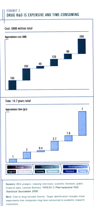
Before the details of the microcalorimeter are discussed, it is important to understand the basic elements of the drug discovery process. In 2001 the Boston Consulting Group (BCG) published a report describing the research and development (R&D) practices of the pharmaceutical industry [1]. Exhibit 2 from the report (see Figure 1-1) indicates that approximately one billion dollars are spent over 15 years to produce a new drug. As a result, even a minor improvement along the drug development

timeline may significantly reduce the amount of money and time needed to bring a new drug to market.

The initial drug discovery process, before the preclinical and clinical trials, consists of four parts: (1.) target identification, (2.) target validation, (3.) lead identification, and (4.) lead optimization [13]. During target identification, biologists identify the proteins, enzymes, hormones, and other elements that affect a particular disease and then isolate the target for further study. After a particular target has been selected, researchers often perform in vivo (in the living subject) animal studies to verify that the target is responsible for a particular disease in target validation. Next, through the use of high-throughput screening (HTS), compounds are individually tested against the target to ascertain their ability to affect the functionality of the target during lead identification. Pharmaceutical companies screen a subset of their proprietary chemical library against the identified target looking for "hits" or successful target-compound interactions. These screenings may encompass hundreds of thousands of experiments in highly automated HTS centers. Finally, after researchers identify potentially promising compound or drug candidates, chemists create new derivative compounds, which are similar to the successful candidates identified in HTS as part of lead optimization. These new compounds are then tested and evaluated for ef-fectiveness. The subject of this thesis, a novel microcalorimeter, is intended to help researchers during steps three and four of the drug discovery process, lead identifica-tion and optimizaidentifica-tion.

Lead identification and optimization techniques can be broadly divided into two groups: conventional methods and label-free methods. Common conventional meth-ods include radioactive and fluorometric techniques [9]. Although there are sev-eral different radioactive and fluorometric methods, the basic process is the same: a radioactive or fluorescent tag is affixed to the compound, which is activated by a successful target-compound interaction. The activated tag is then screened by an optical detector. However, the addition of this label may adversely affect the target-compound reaction. As a result, HTS results will include both false positives and false negatives.

EXHIBIT 2

DRUG R&D IS EXPENSIVE AND TIME-CONSUMING Cost: $880 million total

Approximate cost ($M) 260 90 120 0 40 205 .. .

K

Time: 14.7 years total

Approximate time (yrs)

1.6

2 0.4

1-7--

-SOURCES: BCG analysis; industry interviews; scientific literature; public

financial data; Lehman Brothers; PAREXEL'S Pharmaceutical R&D

Statistical Sourcebook 2000.

NOTE: Cost to drug includes failures. Target identification includes initial

experiments that companies may have outsourced to academic research institutions.

Figure 1-1: A graphic depicting the money and time required to successfully bring a new drug to market. Courtesy of the Boston Consulting Group [1].

165 ---Time: 14.7 years total Aprxmt tm ys

Because of the interference of radioactive and fluorescent tags in target-compound experiments, the current trend is to create and develop label-free detection schemes. Gad et al reports that these new label-free methods include optical, chemical, elec-trical, and acoustic methods [9]. In addition, calorimetric methods have been im-plemented in label-free technologies [7]. However, each of these label-free methods has distinct disadvantages that need to be overcome before their widespread use is adopted in the pharmaceutical industry. Since we employ calorimetric methods to measure target-compound reactions, it is important to understand the advantages and disadvantages of calorimetry.

1.2

Calorimetry

Calorimetry has long been used to further the understanding of materials and their properties, and this section will briefly address the difference between heat and tem-perature, the history of calorimetry and common applications, and finally different calorimeter classifications. As its Latin root suggests, calorimetry involves the study and measurement of heat. It is not, however, the study and measurement of temper-ature. Temperature is an intrinsic property, a thermodynamic state variable, whose units are Kelvins. Heat, on the other hand, is contained in molecular translation, ro-tation, and vibration, and its units are Joules. For example, as water boils heat must continually be fed to the water to maintain the boiling temperature; therefore tem-perature, but not heat, is constant. The purpose of a calorimeter is to measure this change in heat, not temperature. Unfortunately, further complicating the distinction between heat and temperature, researchers commonly publish calorimetric results, not as a measure of heat but as a temperature change, perhaps using Equation 1.1

(making several assumptions in the process, most importantly that the experiment occurred at constant pressure), where H is heat, m is mass, Cp is the specific heat, and T is temperature. It can be misleading to report calorimeter data as a temper-ature change because the tempertemper-ature is dependent upon the mass of the substance, which makes it difficult to compare one system to another. To avoid this confusion,

this thesis will report calorimetric measurements as heat, not temperature.

H2 - H1 = mCp(T2 - T) (1.1)

Calorimetry was born in the latter half of the 18th century. Some of the earliest

known calorimetric experiments were conducted by Joseph Black in 1760 [25]. Since its invention, calorimetry has been applied to several different fields, including: phase transition detection; medicinal purity detection; heat capacity determination; and thermal stability measurement of metals, alloys, inorganic and organic materials, biomolecules, medicines, and biomaterials [21]. Japanese researchers recently built a nano-watt sensitive calorimeter to measure the phase transitions of micrograms of

palmitic acid (C15H31COOH) [23].

Calorimeters can be characterized by their measuring principle and mode of opera-tion [11]. There are three measuring principles: heat conducopera-tion, heat accumulaopera-tion, and heat exchange methods. In heat conduction calorimeters, the heat generated from the sample is conducted away to a sensor, a thermopile, for example. Heat accumulation calorimeters allow the temperature of the system to fluctuate with the sample. Heat exchange calorimeters share heat between the sample and surroundings. There are also three modes of operation for calorimeters: isothermal, isoperibol, and adiabatic. In isothermal calorimeters there is no temperature gradient between the sample and the surroundings and both are held constant. An isoperibol calorimeter keeps the temperature of the surroundings constant (e.g. through a shield) while allowing the temperature of the sample to vary. In an adiabatic calorimeter no heat is exchanged between the sample and the surroundings. The calorimeter that is the focus of this thesis is a hybrid heat conduction/accumulation isoperibol calorimeter. The next section will discuss the specific application of calorimetry to drug discovery.

1.3

Calorimetry Application: Drug Discovery

Although calorimetry has been used since the 1 8th century, its application to

applied calorimetry to study biochemical systems [18,20,22,24]. Currently, there are

several commercially available calorimeters and the use of calorimetry to aid drug discovery is becoming commonplace.

Biophysicists use calorimetry in drug discovery to experimentally determine three

key properties of the target-compound interaction: (1.) the binding enthalpy (AHb),

(2.) the equilibrium binding constant (Kb), and (3.) the reaction stoichiometry

(u) [17].

The binding enthalpy (J) indicates the amount of energy that is released or ab-sorbed in a chemical reaction if it occurs at constant pressure. The calorimeter of this thesis operates at constant pressure. A positive value for AHb denotes an energy absorption or endothermic reaction, while a negative value for AHb denotes an energy release or exothermic reaction.

The equilibrium binding constant (M-1), reveals the direction a chemical reaction tends. Kb is mathematically defined in Equation 1.2. The bracket notation indicates concentration, where A is the compound, B is the target reactant, and AB is the target-compound product. For example, if Kb is greater than unity, than the product

AB (see Equation 1.3) is favored and if Kb is less than unity, the reactants A and B

are favored. Hence, Kb reveals how tightly the drug compound binds to the target molecule. The equilibrium dissociation constant (Kd = 1-) is often reported instead

in the literature. The equilibrium dissociation constant is a metric that shows the necessary concentration or molar amount of one reactant (compound) to produce 50% of the product. A low Kd value indicates a tight binder because less compound is needed to occupy available binding sites on the target. Hence for a tight binder, more energy would be needed to removed the compound from the target molecule.

[A]

Kb = (1.2)

[B] [AB]

A + B ' AB (1.3)

sites on the target. Because the target only has discrete binding sites, the reac-tion stoichiometry value will only assume positive integer values. (As a side note, calorimetry is also used to determine the purity of various substances; the deviation of the fitted model n value from the known n value is an indication of the impurity of the substance.) Researchers will then use these three parameters (AHb, Kb, and n), as mentioned previously, during lead identification and lead optimization to quantify and gauge the effectiveness of a potential drug candidate for their specific application. However, currently available calorimeters are relatively slow; it may take over two hours to perform an experiment with one target and one compound to extract data for AHb, Kb, and n. As a result, only a very small subset, approximately 20-30, of HTS hits will be screened by calorimetric methods. Hence, there is a need to design calorimeters that are highly sensitive, fast (i.e. low time constant), and potentially measured in parallel.

The remainder of the thesis will discuss the design, characterization, experimen-tation, and conclusion of a custom built calorimeter.

Chapter 2

Calorimeter Design

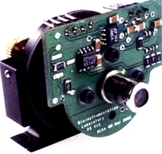
This chapter contains the functional requirements for our calorimeter, a review of the performance of current calorimeters, and a discussion of the design of key components of the calorimeter. Figure 2-1 is a picture of our calorimeter system.

2.1

Functional Requirements

We have identified four key functional requirements for the microcalorimeter and corresponding metrics listed in Table 2.1.

Now each functional requirement will be discussed. The primary reason to have a sensitive calorimeter is to be able to perform experiments with very low concentra-tions (- pM to mM) of both the target and drug compound because both targets and compounds are expensive. The second functional requirement, low reactant vol-ume, is also an attempt to minimize the cost of experimentation. For example, Pfizer currently uses the MircoCal VP-ITC MicroCalorimeter, which requires a combined

Table 2.1: A summary of the key functional requirements and their corresponding metrics for the microcalorimeter.

Functional Requirement Metric

High calorimeter sensitivity 8.4 pJ

Low reactant volume < 20 tpL

Experimental variance (repeatability) < 10%

Figure 2-1: A picture of the complete calorimeter prototype.

volume value of approximately 1.4 mL and has a quoted sensitivity of 6.3 + 0.63

MJ [2]. In essence, the volume and sensitivity functional requirements require the

microcalorimeter prototype to be as sensitive as the MicroCal instrument while using a reactant volume that is almost two orders of magnitude less. The third functional requirement, experimental variance, is crucial to ensure that the calorimeter is re-peatable. Although a variance of 10% may appear high, the resulting variance in the equilibrium binding constant Kb for different compounds may be as much as several orders of magnitude. Hence, a variance of 10% is adequate to distinguish one po-tential drug compound from another. Finally, perhaps the most difficult functional requirement is the baseline calorimeter thermal drift. Is it critical to decouple the calorimeter as much as possible from its environment. To require that the baseline

Table 2.2: A summary of both academic and industry calorimeters and their core technology used and their respective performance.

Calorimeter Technology Volume Resolution

MicroCal VP-ITC [2] thermopile 1.4 mL 6 pJ

TA Instruments Nano ITC [4] thermopile 1.0 mL 0.1 ,/J Palo Alto Research Center [3] custom thermistor 500 nL 2 pJ

Cooper et al. [15] custom thermopile 720 pL 13 nW

Hunter et al. [8] liquid expansion 2 pL 4 uJ

Baudenbacher et al. [26] thermopile -50 nL 132 nJ

drift over a two-hour period by the same as the sensitivity of the instrument, 8.4 PJ, requires an extremely sensitive instrument.

2.2

Current Calorimeter Research

There is active research, both in academia and industry, to develop better calorime-ters. Table 2.2 lists several different calorimeters and some of their performance characteristics. This table shows that most of these calorimeters employ electrical methods (i.e. temperature-voltage or temperature-resistance relationships) to detect heat. Due to the nature of calorimetry, which requires measuring a heat signal over a given period of time, it is extremely difficult to remove low frequency noise (< 1 Hz) because calorimetric measurements are low frequency measurements. This low frequency noise, often called 1/f noise or pink noise, commonly appears in nature. Our prime motivation to develop a resonant heat sensor as a part of the calorimeter was to move the heat measurement to a frequency much greater than the pink noise region (hundreds of Hz). The goal was to use the resonant peak of the sensor as a narrow band-pass filter to remove as much noise as possible.

In addition, although commercial calorimeters predominantly use electrical meth-ods to detect heat, there are several examples of non-electrical techniques that have been implemented to transduce a heat signal. For example, researchers have built calorimeters using bimetallic metal cantilevers to measure heat outputs. [6]. This thesis documents a prototype calorimeter that uses the thermal expansion of a beam combined with the dynamics of a vibrating ribbon as a measurement transducer.

2.3

Calorimeter Components

There are five main subsystems of the microcalorimeter: the novel heat sensor, posi-tion sensor, temperature controlled vacuum chamber, software, and the syringe pump.

2.3.1

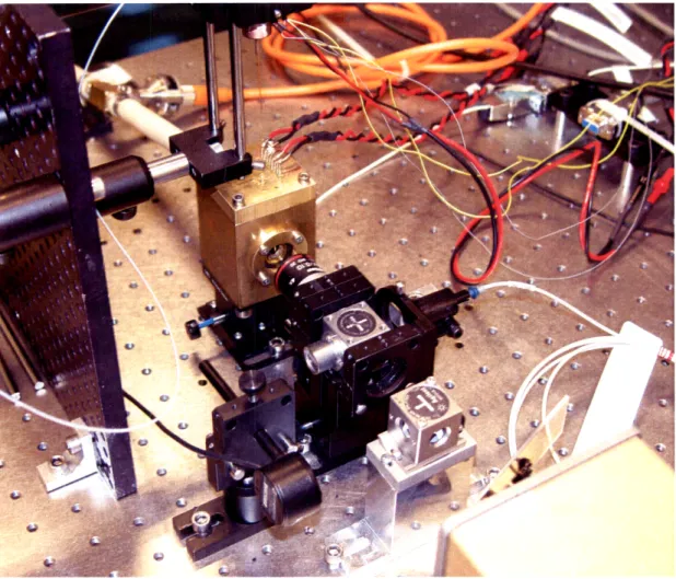
Novel Heat Sensor

The heat sensor combines thermal expansion and the dynamic response of an oscillat-ing ribbon to transduce the signal from a heat event. Figure 2-2 depicts a schematic of the sensor and a picture of a prototype sensor. An aluminum beam is glued to a quartz reaction chamber, which in turn has a small (20 pm by 370 pm cross section) amorphous steel ribbon attached to it. The ribbon is threaded through two flat glass capillaries and then attached to the beam using UV-curing glue to ensure electrical and thermal insulation between the ribbon and the aluminum beam. The ribbon is electrostatically actuated at a fixed frequency. Similar to some amplitude modulation techniques, the driving frequency is intentionally chosen to be slightly off resonance to increase the sensitivity of the sensor (i.e. operate on the steepest slope).

The heat sensor was modeled as a vibrating string system. Although the vi-brating string system is one of the most well characterized systems studied, it has proven difficult to model the heat sensor with sufficient detail to match phenomena observed experimentally. For example, consider Equations 2.1, which represent the fundamental frequency of a vibrating string, thermal expansion, Hooke's law, and axial stiffness of a beam relationships respectively. Clearly there are several major assumptions built into these equations including that there is only planar vibration, there is no damping, the axial stiffness of the aluminum beam is much greater than the axial stiffness of the ribbon, the ribbon operates purely in the elastic region, etc. However, for a first order approximation these appear to be reasonable assumptions for this heat sensor.

Figure 2-2: A schematic and actual picture of the heat sensor. 1 F

f

Equation 2.2 (derived from Equation 2.1 computes the frequency change due to a temperature change of the aluminum beam (see Equation 2.2), where Af refers to the change in frequency, L is the length of the vibrating ribbon, A is the cross-sectional area of the ribbon, E is the Young's modulus of the ribbon, a is the coefficient of thermal expansion of the aluminum beam, AT is the temperature change, and F refers to the tension in the ribbon (specifically F refers to the tension in the ribbon before the temperature is increased). During the assembly of the heat sensor, the

ribbon is tensioned to approximately 30 mN before being glued in place. However, Equation 2.2 predicts that the frequency change scales with the square root of the temperature change, and this behavior is not observed experimentally.

f = f2 -1 =

L

While an analytical model describing the behavior of the sensor has yet to be developed, a number of qualitative statements about the sensor can be made. First, an exothermic reaction increases the temperature of the aluminum beam, which then expands and increases the tension of the ribbon. As a result, the damped natural frequency increases. Likewise, an endothermic reaction absorbs heat and the tem-perature of the aluminum beam decreases, which then constricts and decreases the tension in the ribbon. As a result, the damped natural frequency decreases. Second, the shape of the sensor output depends on what side of the resonant peak one oper-ates. If the sensor is operated at a frequency less than the damped natural frequency, an exothermic reaction will cause a decrease in output amplitude as the resonant frequency increases. Similarly, if the sensor is operated at a frequency greater than damped natural frequency, an exothermic reaction will cause an increase in output amplitude as the resonant frequency increases. The opposite relationships exist for endothermic reactions.

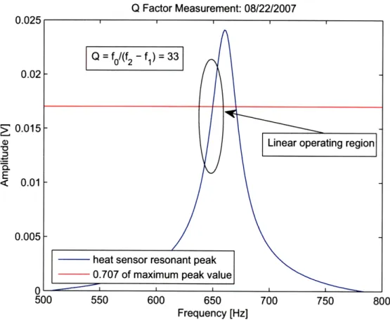
While a qualitative description of the system is helpful, a quantitative method of characterization is also needed to steer the design of the senor. Since the heat sensor operates near resonance, we can use the quality (Q) factor to drive the design of the sensor. The Q factor is defined in Equation 2.3, where fo is the resonant frequency and Af is the bandwidth of the resonant peak that corresponds to half of the maximum energy in the vibrations or -3 db (.707) of the maximum amplitude of the resonant peak. The frequency response of the heat sensor was measured and a Q factor of 33 was calculated (see Figure 2-3).

Q

f

Q Factor Measurement: 08/22/2007 I I --U.ULO 0.02 0.015 E < 0.01 0.005 0

heat sensor resonant peak 0.707 of maximum peak value

Linear operating region

500 550 600 650 700 750 800

Frequency [Hz]

Figure 2-3: The frequency response of a heat sensor in air and the calculated Q value. In order to increase the sensitivity of the heat sensor, the Q factor must be max-imized. The Q _{factor is inversely proportional to the damping ratio (. Hence, to}

maximize Q, _{( should be minimized. The main contributor to damping in this}

sys-tem is due to viscous drag. Rugar et al suggest that to increase the sensitivity of their resonant cantilever, one can reduce the losses due to viscous drag by placing the sensor in a vacuum chamber [5]. In a second iteration of the calorimeter, we built a vacuum chamber to house the heat sensor. As a result, the measured Q factor increased more than an order of magnitude, to 464. The slope of the linear region can roughly be calculated by Equation 2.4, where m is the slope and Ao is the amplitude at the damped natural frequency. Hence, the slope is proportional to the Q factor, so we should expect approximately an order of magnitude increase in sensitivity by putting the heat sensor in a vacuum (It will actually be more because the ratio AO

fowill only increase with increasing Q.). will only increase with increasing Q.).

Q = fO_/( -2 -f ) = 33 -/ r\ r\rr~

Ao - 0.707Ao 0.586AoQ (24)

m= Af = f(2.4)

fo

2

2.3.2

Position Sensor

As mentioned previously, the custom heat sensor relies on thermal expansion and the dynamic response of an oscillating ribbon to transduce a heat input. In order for the heat sensor to function, a position sensor must be able to adequately capture the dynamic response of the vibrating ribbon. Initially, a custom confocal sensor with subnanometer linear position resolution, designed and built in the BioInstrumentation Laboratory [10], was used to characterize the dynamic response of the ribbon (see Figure 2-4).

Figure 2-4: A picture of a prototype confocal position sensor previously designed and built in the Bioinstrumentation Laboratory.

However, due to the heat output of the confocal senor's electronics (problematic because of its proximity to the heat sensor) and the sensor's limited dynamic range, later prototypes used an Agilent Laser Interferometer Position Measurement System. There are several different interferometer types and configurations, the Michelson Interferometer being the most common [12]. However, the majority of these methods are amplitude-dependent, and any laser power fluctuations will increase measurement

error. Furthermore, because of the energy sensitive nature of the heat sensor, it is important to limit the amplitude of the light source as much as possible while still maintaining a signal. Because of these shortcomings, a heterodyne interferometer was chosen instead to characterize the dynamic response of the oscillating ribbon.

A heterodyne interferometer is a frequency dependent measurement technique. Basically a laser produces a beam embedded with two different frequencies a few MHz apart, one polarized horizontally and the other vertically. Then an interferometer divides the beam into two single frequency beams. One becomes a reference and reflects from a stationary mirror, and the other reflects off a mirror affixed to the moving entity of interest. The single frequency beams then recombine and optical detectors measure the resulting frequency difference between the two beams. This difference is then compared to the original frequency difference and the velocity of the moving entity is calculated using the Doppler effect (see Equation 2.5 where fo is the observed frequency, c is the speed of light, vo is the velocity of the observer, and fs is the frequency of the source). Once the velocity has been measured, the position can be determined by integrating the velocity signal with respect to time (see Agilent Interferometer System manual).

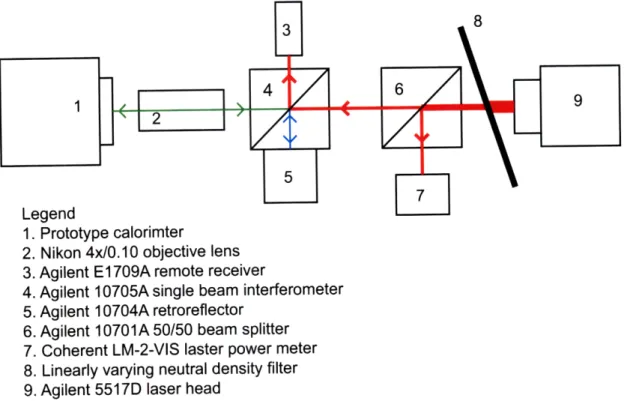
fo

Figure 2-5 displays the optical path of the interferometer sensor. The Nikon objective lens is used to focus the 6 mm beam onto the 370 pm wide ribbon. Nominally the laser head produces a 320 pW beam, but a neutral density filter only allows approximately 2% of the light through. Then a 50/50 beam splitter cuts that in half, so the laser power meter will generally report a laser power of 3-6±0.01IPW. However, the interferometer should remove another 50% of the light intensity as it separates the two frequencies into separate beams. As a result, the incident laser radiation on the heat sensor should be less than 1.5 - 3.0 ± 0.01pW. The goal is to minimize the incident radiation on the heat sensor from the position sensor as much as possible, while still maintaining a signal. Although much of the the laser power will be reflected

by the vibrating ribbon, some of the radiation will be absorbed and be a source of error in the measurement.

1. Prototype calorimter

2. Nikon 4x/0.10 objective lens 3. Agilent E1709A remote receiver

4. Agilent 10705A single beam interferometer 5. Agilent 10704A retroreflector

6. Agilent 10701A 50/50 beam splitter 7. Coherent LM-2-VIS laster power meter 8. Linearly varying neutral density filter 9. Agilent 5517D laser head

Figure 2-5: A schematic of the optical pathway involved in measuring the displace-ment of the vibrating ribbon.

In addition to reading the position of the vibrating ribbon, an algorithm is needed to fit a function to the raw data. A Labview curve fitting algorithm is used to compute both the amplitude and frequency of the vibrating ribbon. Also, the particular Agilent interferometer system used reports a linear position resolution of 0.3 nm and has a maximum sampling rate of 20 MHz.

2.3.3

Temperature Controlled Vacuum Chamber

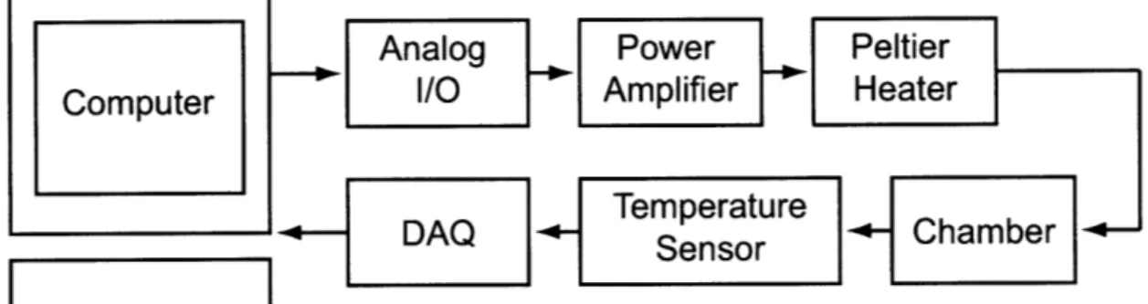
Another critical component of the calorimeter system is the temperature controlled chamber. Initially, a temperature controlled chamber was built to isolate the calorime-ter from the environment. Lacalorime-ter a vacuum chamber was added to increase the sensi-tivity of the calorimeter. Figure 2-6 shows a block diagram of the components used in the temperature controller. A Dell Precision 390 implements a proportional-integral

(PI) controller in Labview software. Data is sent from the computer to an Agilent 34970A Data Acquisition/Switch Unit via a GPIB interface. An Agilent 34907A Multifunction module (plugged into the switch unit), with on-board digital-to-analog converters (16 bit resolution), outputs an analog signal to a Techron 8803 Power Sup-ply Amplifier. Twisted cable connects the power amplifier to a peltier heater. The peltier heater is connected to the temperature chamber by thermal paste and UV glue. The resistance of the temperature sensor is then read by an Agilent 34901A 20-Channel Armature Multiplexer module (plugged into the switch unit). This switch unit has on-board analog-to-digital converters whose bit count is a function of the integration time or the number of power line cycles (PLC). In this controller the tem-perature sensor is sampled at 2 Hz with an integration time of 10 PLC, which leads to 24 bit resolution.

Analog

Power

Peltier

Computer

I/O

Amplifier

Heater

Temperature

C

+- DAQ

_D

~

Sensor

Figure 2-6: A block diagram of the temperature controlled chamber.

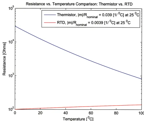
It is important to note, however, that this design has evolved over time. Initially an Pt 100 Q resistance temperature detector (RTD) was used as the temperature feedback sensor (Omega SAI-RTD 4W 80 see www.omega.com). In RTDs, resistance and temperature are linearly related over large temperature ranges, and because of their low nominal resistance, are typically used in a four-wire configuration. This re-moves the lead resistance from the measurement, which could potentially account for as much as 5% measurement error. In addition, RTDs generally have greater absolute temperature accuracy compared with other temperature sensors. However, in a sec-ond iteration of the calorimeter a thermistor (Omega 44031 10k see www.omega.com) was used as the temperature sensor because of its increased sensitivity. Thermistors

are highly non-linear sensors that exhibit a decaying exponential relationship be-tween resistance and temperature. However, near room temperature the slope of the resistance-temperature relationship is steeper for a thermistor than an RTD (see Figure 2-7). _{As a result, the resolution of a thermistor is greater than the}

resolu-tion of an RTD by an order of magnitude. On the other hand, thermistors' absolute temperature accuracy is poor compared to RTDs. Fortunately, in this application the absolute temperature is not critical, but rather the resolution of the sensor and the ability of the temperature controller to minimize steady state error. In addition, because we are not overly concerned with absolute temperature performance, the re-sistance measurement is taken in the two wire configuration, so thermistors were used as temperature sensors.

2.3.4

Software

Labview 8.5 and MATLAB were used to organize, control, and analyze the calorimeter system. Figure 2-8 displays a screen shot of a Labview program used to measure the frequency response of the heat sensor.

One critical component with respect to software was the necessity to program a deconvolution algorithm. This is necessary to compute the actual heat generated by a reaction. Figure 2-9 displays a simple block diagram of a general system with two additive noise sources. Typically the input is known and the engineer is left to determine either the output or system response; however, in this case, the input is the unknown. Furthermore, the input is a function of the nature of the interaction between the target and compound. Hence, it becomes necessary to predict the input based on knowledge of the impulse response of the system and the measured output. This input can then be predicted through deconvolution. Referring again to Figure 2-9, the block diagram assumes that the inputs, outputs, etc. are in the Laplace domain. As a result, Equation 2.6 shows the relationship between input, output, plant, and noise.

10 104 E -1 2 CI

Resistance vs. Temperature Comparison: Thermistor vs. RTD

0 20 40 60 80 100

Temperature [oC]

Figure 2-7: A semilog plot comparing the resolutions (sensitivities) of thermistors and RTDs. The curves were generated using the Steinhart-Hart (thermistor) and Callendar-Van Dusen (RTD) equations. Also the slopes have been normalized for the nominal resistance of the sensor, which shows that the thermistor is approximately an order of magnitude more sensitive than the RTD.

Now if you assume that the contribution due to noise is minimal Equation 2.6 becomes:

Input(s)System(s) = Output(s) (2.7)

Now we can solve for the input as a function of the output and the system impulse response as seen in Equation 2.8, which is a method for calculating an unknown input through deconvolving the system impulse response from the output. As the equation shows, in order to compute the input, the output and system impulse response must be known. The output is measured by the laser interferometer system. The system impulse response was measured by applying a 400 pJ pulse over one second through a

- Thermistor, Iml/Rnominal = 0.039 [1/ OC] at 25 OCI

400 Q surface mount resistor. The system response was approximated as a first order system with a measured time constant of approximately 70 seconds. It is reasonable to assume a one second heat pulse sufficiently approximates a true impulse input because its duration was less than 2% of the measured time constant.

Input(s) Output(s) (2.8)

System(s)

It is essential that this input can be successfully calculated. After the input is known, a curve fitting algorithm, often a Marquardt algorithm, is needed to calculate the thermodynamic data (the binding enthalpy AHb, the equilibrium binding constant Kb, and the reaction stoichiometry n for the reaction). The details of this process can be found in two isothermal titration calorimetry review articles listed in the bibliography [14, 16].

2.3.5

Syringe Pump

The last major item that is needed to successfully perform experiments is a syringe pump that delivers both reactants to the reaction chamber inside the calorimeter. Figure 2-10 shows an early syringe pump prototype. Two linear actuators, a Zaber T-LA60A and a Parker 404500XRMP stage driven by a Zeta 57-83 stepper motor, are co-mounted on the same axis. The Zaber actuator drives the piston of a Hamilton 50 yL syringe and the Parker stage moves the entire syringe. As a result, the syringe pump can simultaneously inject reactants while withdrawing the syringe from the calorimeter reaction chamber. In order to ensure repeatability, a simple injected volume study was performed, and the syringe pump consistently delivered 9.5±0.2

,pL when aiming for a 10 pL injection.

However, initial experiments revealed that the syringe pump provided a direct connection between ambient temperature fluctuations and the stable temperature controlled chamber. As a result, the heat transfer was often so large that it masked any heat signal produced from the actual reaction. To combat this problem, a second syringe pump was built to reduce these coupling effects. Although it functioned better

than the initial prototype, more work needs to be done to fully mitigate the influence of the external syringe pump coupling ambient temperature fluctuations to the stable reaction chamber. The goal should be to minimize temperature gradients between the syringe pump and reaction chamber as much as possible.

Figure 2-8: The front panel of a Labview program used to measure the frequency response of the heat sensor.

Noise

Noise

Input

Figure 2-9: A basic block diagram of a system that includes two potential noise sources.

Figure 2-10: An early syringe pump prototype consisting of two linear actuators, a Hamilton syringe, and a custom pulled borosilicate pipette.

Chapter 3

System Characterization

In order to verify the design of the calorimeter and its constintuent components, several experiments were performed to characterize their behavior. This chapter will discuss the characterization of the heat sensor, temperature-controlled chamber, and the deconvolution algorithm. It is necessary to characterize the system before real experimentation can begin.

3.1

Heat Sensor

Despite the difficulty of accurately modeling the system mentioned previously, it is critical that the system performance is repeatable and that the system can be cal-ibrated. While developing the theory for the heat sensor, we assumed that in the operating region off resonance that there is a linear relationship between heat in-put and measured amplitude. Figure 3-1 verifies this crucial assumption. A resistive heater (a 400 Q surface mount resistor) was placed in the calorimeter's reaction cham-ber and two one-second heat pulses at the following energy levels were performed: 500 p J, 1000 p J, 1500 IiJ, 2000 p J, 5000 pJ, and 10000 jpJ. The sixth measured point at 10000 11J qualitatively deviates from the clear linear relationship for the other five

points. This is due to the 10000 pJ energy pulse moving the calorimeter response out of the linear region of the resonant peak. Hence, one potential disadvantage of this resonant sensing technique is that the dynamic range is limited to energies that

will remain in the linear portion of the resonant peak. A fitted curve for the first five points is seen in Equation 3.1, where a = 0.28 [y] and b = -11 [,aV] and an R2 = 1.0. This result does confirm that the linear assumption made is accurate and provides a simple method to calibrate the system. However, note that the b or y-intercept term is not zero. We should expect zero output for zero input, but noise adds error to the measurement. 2 Z- 1.5 0. a o0 -' 1 0 0.5 x 10-3 Calibration: 08-06-2007 2000 4000 6000 8000

Energy Pulse (microJ)

10000

Figure 3-1: This plot shows calibration experiments using

the linear response of the calorimeter due to several a resistive heater.

y = ax + b _(3.1)

After it was confirmed that the linear operating region assumption was valid, the frequency response of the system was measured as a function of pressure to see the affect of the vacuum chamber on damping. Figures 3-2 and 3-3 show the results for two different electrostatic stimulating voltages. Both of these plots reveal an

esting unanticipated behavior. As expected, the resonant peak becomes sharper and narrower as the pressure in the vacuum chamber decreases. However, the resonant frequency of the system initially increases slightly (moves to the right) and then sig-nificantly decreases (moves to the left). Theoretically, in a second order system as the damping ratio ( approaches zero, the damped natural frequency approaches the natural frequency of the system as seen in Equation 3.2, where wd is the damped natural frequency and w, _{is the natural frequency. We determined that as the}

pres-sure in the chamber decreased, the laser radiation from the interferometer began to affect the performance of the sensor. As the pressure decreases, the convective heat transfer coefficient decreases and the ribbon can no longer dissipate the incident laser radiation. As a result, it absorbs energy, heats up, expands, decreases the tension in the ribbon, and lowers the resonant frequency.

Improvement in Q with Vacuum (3.6V rms Stimulation Voltage)

... _{. . . .. . . .. .. .} . t. D 0) E 2 S 4) C. - U 1000 Pressure (Torr Frequency (Hz)

Figure 3-2: This plot charts the frequency response of the calorimeter as a function of pressure.

Wd = WnV1 _ '2 (3.2)

Another interesting behavior seen in the frequency response of the ribbon as a function of pressure is seen in the nonlinear behavior of Figure 3-3. As the the

trostatic voltage is increased, the system response qualitatively looks like a crashing wave. This behavior has been observed previously and can be modeled [19]. There was an initial attempt to try and operate on the knife edge of the resonant peak as it snaps out of resonance, but proved too difficult to keep the system in this operating range.

Improvement in Q with Vacuum (10.8V rms Stimulation Voltage)

x 104 ... I-0) e E 2 S E A 7O YU o 1000 U Pressure (Torr) Frequency (Hz)

Figure 3-3: This plot shows the nonlinear response of the heat sensor when the forcing amplitude is large.

Now that the frequency response has been measured as a function of pressure, the sensitivity improvement can be quantified. Figure 3-4 compiles all of the frequency response traces of Figure 3-2 into one normalized plot. Furthermore, only the linear portions of the resonant peak are shown. This plot clearly shows the improvement in sensitivity as a function of decreasing pressure, and it predicts a sensitivity increase of approximately an order of magnitude. This also corresponds with the earlier doc-umented improvement of the measured Q factor for the vacuum chamber calorimeter versus the atmospheric calorimeter.

Finally, Figures 3-5 and 3-6 document the improvement in sensitivity using a resistive heater for calibration. In Figure 3-5, 100 /J one-second pulses are injected at 30-second intervals. This data was taken at atmospheric pressure. The plot shows

0.9 0.85 -o .1. 0.8 E 0.75 E 0 0.7 - 0.65 N E 0.6 o z 0.55 0.95

Calorimeter Sensitivity: Linear Operating Region

0.96 0.97 0.98 0.99

Normalized Frequency (Omegad/Omega)

Figure 3-4: This plot displays normalized data representing the linear region of op-eration for the data shown in Figure 3-2.

that the peaks are roughly 45 interferometer units in height with an approximate signal-to-noise ratio of 20. Figure 3-6 displays data obtained at an approximate pressure of 1 Pa and with 10 pJ pulses at 60-second intervals. The height of the peaks are roughly 60 interferometer units with a approximate signal-to-noise ratio of 10 (for higher frequency noise). Hence, as expected we see an order of magnitude improvement in the sensitivity of the calorimeter. However, this increased sensitivity reveals a significant underlying thermal drift. In order to successfully resolve energy events on the order of 10 4/J (or near the required metric for sensitivity), this thermal

drift needs to be minimized.

i

,

/

Measured Output of 100 microJ, 30 sec Period Input Pulses bu 45 40 35 30 . 25 E 2 20 S15 10 5 0 -E 8900 9000 9100 9200 9300 9400 9500 9600 Time (sec)

Figure 3-5: This graph shows the calorimeter responses due to a programmed 100 jJ

pulses (over one second) from a resistive heater in the reaction chamber. This data was taken before the vacuum chamber was built.

3.2

Temperature Control

It was critical to actively control the temperature of the chamber to isolate the heat sensor from the environment. Figures 3-7 and 3-8 show the measured chamber step response and temperature locations. The temperature chamber was approximated as a first order thermal system and the measured time constant was approximately 1000 seconds, which is mainly due to the large thermal capacitance of the aluminum box. In this application, not speed, but rather steady state error is important, so the large time constant is not a problem. However, a big concern with respect to controllability of the system is time delay. In subsequent experiments when the feedback temperature sensor was located on the interior wall (wall thickness is 10 mm) of the aluminum chamber, there was approximately a 5-second time delay between the peltier heater and the temperature sensor. This delay led to control instabilities, manifested by

Figure 3-6: This demonstrates that the sensitivity of the microcalorimeter roughly increases by an order of magnitude when placed in a vacuum chamber. However, the effects of thermal drift appear to be more evident in the reduced operating pressure. The pulses are 10 pJ each with a period of 60 seconds.

exponentially increasing oscillations about the reference temperature. As a result, in subsequent designs the temperature sensor was located as close to the peltier heaters as possible. This was done by drilling a hole in the chamber wall such that the material thickness between the peltier heater and the sensor was less than 1 mm.

A PI controller was implemented in Labview to control the temperature chamber. The integral term is necessary to minimize steady state error as much as possible. Theoretically the integral term will completely remove any steady state error in a stable system. Unfortunately this is not possible in this situation due to measurement noise. During the initial prototypes the controller was tuned manually using common PI controller tuning methods. However, in the latest prototype the autotuning feature of the PI controller Labview vi was used to tune the controller. Figure 3-9 shows the

Plant: Heating @ IV - 4/1Q21007

Figure 3-7: Measured step response for various temperature sensors due to a 1V voltage across two peltier heaters located beneath the aluminum box (see Figure 3-8 for temperature sensor locations).

temperature performance of the final temperature chamber prototype. The steady state performance over a 24-hour period was measured to be 25.0000+0.0001320_C

(la).

In addition to serving as an isolator from the environment, the temperature cham-ber also serves as a vacuum chamcham-ber. As mentioned previously, in order to increase the sensitivity of the heat sensor a vacuum was used to minimize the damping of the vibrating ribbon due to air friction. Two o-ring grooves were machined into the cham-ber: one to receive a circular glass window and the second to allow an easy exchange of different heat sensors. In addition, a 1/4 inch NPT tapped hole provides access to the vacuum pump. A Welch Duoseal 1400 Vacuum Pump draws the vacuum in the chamber (continuously running), whose pressure is measured by a Teledyne Hastings

26 25 0 O 24 0e23 'u P-

23

Figure 3-8: The first prototype of the temperature controlled chamber. The colored squares refer to temperature sensor locations that correspond to the MATLAB plot measured step response (see Figure 3-7). The blue and green sensors are inside the box, the red sensor is in between the two peltier heaters (outside the box), and the yellow sensor is measuring the ambient temperature fluctuations.

Model 2002 Dual Sensor Vacuum Gage (24 bit analog-to-digital converter resolution). The pump is capable of drawing a vacuum = _{1 Pa. The operating pressure can be}

changed by manually opening a bleeder valve. Surprisingly a compliant vacuum line and rubber pad were all that was necessary to decouple the mechanical vibrations of the pump from the chamber.

3.3

Software

A deconvolution algorithm was subsequently written in MATLAB to determine the experimental input of the calorimeter. To verify that the algorithm was functioning

Temperature Controlled Chamber: Measured Performance 50 100 150 200 Time [sec] I I I I 5 10 15 20 Time [hours]

Figure 3-9: A plot showing the measured temperature stability for the calorimeter chamber showing both the transient response (240 seconds), as well as the steady state response (for a 24 hour period).

correctly, three different waveforms were programmed into an Agilent 33220A 20 MHz Function/Arbitrary Waveform Generator to achieve a specific power profile, dissipat-ing heat through a 400 Q resistor. Figures 3-10, 3-11, and 3-12 show the programmed waveform as well as the calculated input using the aforementioned programmed algo-rithm. The figures show good correlation between the programmed input waveform and the calculated input, especially for the half-sine profile.

L) o , E:. I--0 25.0005 F? S25.00025 A 25.0000 E 24.99975 I-24 A99 I 0 I I 0Y--"

Deconvolution Algorithm Test #1: 07-25-2007

110 120 130 140 150 160 170

Time (sec)

Figure 3-10: This plot shows the response 10-second ramp heat input from a resistor.

of the calorimeter due to a programmed

x 10-3 Deconvolution Algorithm Test #2: 07-25-2007

I I I I I I I I I

-

Sprogrammed waveform input

I I I I I I I

90 100 110 120 130 140 150 160 170 180

Time (sec)

Figure 3-11: This plot shows the response of the calorimeter due to a programmed 20-second ramp heat input from a resistor.

0.5 o = 0 -0.5 -1 x 0 3 Dcnouto loih es 20-520

id

3 2.5 2 1.5 1 0.5 0 -0.5

x 10-3 Deconvolution Algorithm Test #3: 07-26-2007

100 150

Time [sec]

Figure 3-12: This plot shows the response of the calorimeter due to a programmed 40-second half-sine heat input from a resistor.

51

programmed waveform input

jl

,

Chapter 4

Experimental Results and

Discussion

This chapter presents several figures that document the quantitative results obtained by actual reactions performed using the calorimeter.

After the system had been calibrated using a resistive heater, experiments were performed to determine the ability of the calorimeter to measure the heat outputs of biological solutions. Initially dimethylsulfoxide (DMSO) concentration mismatched solutions were used to measure the heat of dilution and the heat of mixing. Figure 4-1 shows the raw output (before deconvolution) of 10 pL of 50% DMSO and water mixed with 10 pL of deionized water. The first two downswings show the syringe pump moving into the reaction chamber: the first downswing displays 10 pL of the first reactant deposited into the reaction chamber; the second downswing displays the loaded syringe with the second reactant; and the peak shows the heat produced when the second reactant was injected into the first. Figure 4-2 displays the decon-volved input of this reaction. Note that this experiment was performed in the initial calorimeter prototype that operates at atmospheric pressure. In the same calorime-ter, another experiment was able to detect the heat produced by a reaction of 10 PL of a 2% DMSO solution mixed with 10 /L of a 3% DMSO solution.

Although the atmospheric calorimeter was able to detect a 1% DMSO mismatch, it still was not sensitive enough to capture target-compound reactions. As a result,

50% DMSO into Water

x 10- 3

0 100 200 300 400 500

Time (sec)

Figure 4-1: This graph shows the solution mixed with 10 pL of water.

600 700 800 900

raw signal produced by 10 pL of 50% DSMO

after the vacuum chamber was built and initially characterized, a round of exploratory reactions were performed. Figure 4-3 contains a plot of a water into water reaction. Similar to previous experiments, 10 pL of water were deposited into the reaction chamber, then the syringe pump returned with 10 AL of water and waited for roughly five minutes, before finally injecting the the second 10 PL of water into the first. The plot only shows the results of the actual water-into-water mixing.

These results are puzzling, but unfortunately they are repeatable. Since this ex-periment was conducted at a frequency less than the damped natural frequency, these results suggest that first water mixing produced heat, then absorbed heat, and finally produced heat. This erratic behavior may be explained by a temperature gradient between the two drops before mixing in combination with significant laser power fluc-tuations from the interferometer system. It has been measured that the laser power

---Deconvolution Algorithm Test #3: 09-06-2007

0 100 200 300 400 500

Time (sec)

Figure 4-2: This chart displays the deconvolved input was calibrated using a resistive heater.

600 700 800 900

of 4-1. The vertical axis (Power)

varies by as much as 50% over a period of 10-20 seconds, so this explanation might prove plausible. However, without more concrete measurements the true cause be-hind the results seen in Figure 4-3 remains unknown. Therefore, despite the order of magnitude increase in sensitivity for the vacuum calorimeter (see Figure 3-6), the vacuum calorimeter has a number of experimental issues that need to be resolved before more real target-compound experiments can be performed.

X 10- 3

---Deionized Water Into ---Deionized Water Reaction: 04-01-2008

50 100 150 200 250

Time (sec)

300

Figure 4-3: This chart contains the raw output of 10 pL of deionized water mixed into 10 /pL of deionized water. This data was taken from the vacuum chamber calorimeter.

3000 2500 ,, D 2000 E 0 C 1500 E 1000 nn 0 o

Chapter 5

Conclusion and Future Work

5.1

Summary

To summarize the current progress made, it will prove beneficial to refer to the func-tional requirements and their associated metrics and compare them with measured results. Table 5.1 displays the functional requirements, metrics, and measured results

to date. Now each measured performance will be briefly discussed.

The resonant heat sensor sensitivity of 10 pJ was near the target metric of 8.4 pJ. This confirms that it is possible to develop non-electrical methods to amplify the heat signal from calorimeter reactions. However, as previously discussed, the measurement was performed using a resistive heater as the heat input, and more work needs to be performed to quantify the sensitivity for real calorimetric experiments using two biological solutions.

Low reactant volume of 19 pL was close to the metric of 20 pL. The present results would suggest an approximate 5% error in volume precision, which would affect the overall repeatability of the instrument. Fortunately, since the syringe pump is controlled by a linear actuator, the dispensed volume can be calibrated and adjusted in software.

Currently, there are no quantitative results for experimental variance because this functional requirement pertains to the variance of actual experiments. Since there are still several issues that need to be resolved before extensive testing commences,

Table 5.1: A summary of the key functional requirements, their corresponding met-rics, and the measured performance of the microcalorimeter.

Functional Requirement Metric Measured Results

High calorimeter sensitivity 8.4 pJ 10±2 pJ

Low reactant volume < 20 pL 19.0±0.4 pL

Experimental variance (repeatability) < 10% N/A Thermal drift (over a two hour period) < 100 /pK >132±5 pK

no repeatability experiments have been conducted.

The last functional requirement, thermal drift, is difficult to directly measure. As shown previously the temperature controller is able to control the temperature of a copper annulus near the sensor within roughly 132 pK over a 24-hour period. However, there are additional heat sources that couple in to the heat sensor. In addition to conduction from the copper annulus to the heat sensor, incident laser radiation and radiation from the vacuum chamber walls affect the baseline thermal drift of the sensor. As a result, the actual thermal drift will be larger than the measured performance of the temperature controller.

In summary, the prototype calorimeter is near meeting three of the functional requirements, but there is still a great deal of work that needs to be performed to have a complete functioning calorimeter system.

5.2

Future Work

In order to further develop the calorimeter so that it can be used to perform real ex-periments, three key areas need to be addressed: (1.) Temperature control/isolation,

(2.) Syringe pump, and (3.) Curve fitting algorithm to calculate thermodynamic data.

As previously documented, the current temperature controller is capable of con-trolling the temperature within roughly 132 pK. However, the effects of other heat sources need to be mitigated. For example, a kerr cell or pockels cell (which, through feedback, could control the laser power so that it is constant) should be placed in the laser pathway. Also, perhaps a secondary temperature controlled chamber could be