HAL Id: hal-01419017
https://hal.archives-ouvertes.fr/hal-01419017
Submitted on 18 Dec 2016
HAL is a multi-disciplinary open access
archive for the deposit and dissemination of
sci-entific research documents, whether they are
pub-lished or not. The documents may come from
teaching and research institutions in France or
abroad, or from public or private research centers.
L’archive ouverte pluridisciplinaire HAL, est
destinée au dépôt et à la diffusion de documents
scientifiques de niveau recherche, publiés ou non,
émanant des établissements d’enseignement et de
recherche français ou étrangers, des laboratoires
publics ou privés.
A VARIATIONAL APPROACH FOR GEOACOUSTIC
INVERSION USING ADJOINT MODELING OF A PE
APPROXIMATION MODEL WITH NON LOCAL
IMPEDANCE BOUNDARY CONDITIONS
Jean-Claude Le Gac, Yann Stéphan, Mark Asch, Philippe Helluy, Jean-Pierre
Hermand
To cite this version:
Jean-Claude Le Gac, Yann Stéphan, Mark Asch, Philippe Helluy, Jean-Pierre Hermand. A
VARIA-TIONAL APPROACH FOR GEOACOUSTIC INVERSION USING ADJOINT MODELING OF A
PE APPROXIMATION MODEL WITH NON LOCAL IMPEDANCE BOUNDARY CONDITIONS.
Theoretical and computational acoustics 2003, Aug 2003, Honolulu, United States. pp.254 - 263,
�10.1142/9789812702609_0023�. �hal-01419017�
A VARIATIONAL APPROACH FOR GEOACOUSTIC INVERSION USING ADJOINT MODELING OF A PE APPROXIMATION MODEL WITH NON
LOCAL IMPEDANCE BOUNDARY CONDITIONS
J.-C. LE GAC AND Y. STEPHAN
EPSHOM, Centre Militaire d'Océanographie, 13, rue du Chatellier, B.P.30316, 29603 Brest Cédex, France - E-mail: [email protected]
M. ASCH, P. HELLUY
Université de Toulon et du Var, ISITV, Avenue Georges Pompidou, B.P.56, 83162 La Valette du Var Cédex, France - E-mail: [email protected]
J.-P. HERMAND
Royal Netherlands Naval College, P.O. Box 10000, 1780 CA Den Helder, The Netherlands E-mail: [email protected]
The adjoint model method of control theory is known to give accurate and efficient data assimilation processes in oceanography and meteorology. However, it has rarely been applied in underwater acoustics for inversion purposes. Based on the back-propagation of the mismatch between observations and their predictions, the adjoint model can produce the corrections to the associated direct forward model input parameters. In this paper, the adjoint of a parabolic equation propagation model with non local impedance boundary conditions at the water sediment interface is used in order to determine an acoustically equivalent representation of the seabed. The bottom is represented by these boundary conditions that play the role of the control parameter.
1 Introduction
Bottom properties are essential in shallow water acoustics for prediction of the transmission losses encountered in sonar applications. In the last decade inversion methods based on signal processing approaches (matched field processing, inversion of broadband signals) have been applied extensively to estimate geoacoustic features of the bottom (see [1,2] for a survey of the state of the art). The optimization techniques that have so far been used within these methods are mostly perturbative approaches based on the iterative adjustment of the input parameters of a forward model. The forward model is run for a great number of input parameter values until the mismatch between the observations (like the spatial structure of the complex pressure field or the temporal structure of the propagated signal) and their predictions is low. This often results in highly computationally intensive methods.
In this paper, we present an alternative technique based on a variational approach coming from the control theory. This technique aims to solve optimization problems based on partial differential equations. The theory is detailed in [3,4]. Variational methods by adjoint modeling are tools that have so far been developed in the framework of inverse modeling of physical systems, in particular in the domains of geophysics and molecular physics. Their use has been generalized especially to meteorology and oceanography for the purposes of data assimilation [5-7], model adjustment [8], data inversion [9-10,11-12] and sensitivity studies [13]. Variational methods have been recently used for acoustic inversion [14-15,22-23]. In [14], we proposed an optimal control approach based on the use of a parabolic equation (PE) propagation model in which a local impedance condition at the water-sediment interface plays the role of the control parameter. The geoacoustic
concept that was used was that of the acoustically equivalent medium. Rather than seeking the geoacoustic parameters in the physical parameter space, we computed the sea bottom conditions in a way that was not directly comparable with a ground truth model but that was sufficient to predict the field of acoustic transmission losses. These first developments and a feasibility study allowed us to demonstrate the controllability of the PE approximation suggesting the variational approach as a rather promising technique for geoacoustic inversion. However, the use of local impedance conditions is rather limited (though realistic in the framework of aerial acoustics [16]), since they can only be used for local reacting media. For underwater acoustics, a downgoing radiation condition must be imposed on the transmitted component of the field since the seabed is penetrable to sound waves, especially at low frequencies. In PE models, this can be done by appending an absorbing layer [17] or alternatively by applying a non local boundary condition (NLBC). This last method that was first formulated and implemented in a finite difference code by Papadakis [18] is rather attractive. Since then, numerous different forms of the NLBC concept have been proposed (see [19] for some references).
In this paper, we apply the NLBC formulation described in [19] to generate realistic boundary conditions and then adopt a generalized form of these NLBC conditions for the rest of the study. In section 2, the inverse continuous physical problem is presented. We define the associated optimal control problem and compute the analytical form of the gradient of the cost function by using the adjoint model of a PE propagation model. The use of the adjoint model and the gradient of a cost function within a gradient based optimization loop is then presented. In section 3, we present some numerical simulations showing the data assimilation of acoustical data for geoacoustic inversion purposes.
2 The continuous problem
The variational approach being new in the framework of geoacoustic inversion, we adopt a rather simple monochromatic matched field processing inverse technique. The acoustical data we thus use (or the observations) are the spatial structure of the complex pressure field measured along a vertical line array.
2.1 The direct forward model
The direct forward model is the standard PE approximation [20]. The model recognized as the Standard PE is given for a harmonic point source of time dependence
)
exp(
−
i
ω
t
in cylindrical coordinates( z
r
,
)
independent of the azimuthal angleθ
:.
0
)
1
(
2
2 2 0 2 2 0∂
+
−
=
∂
+
∂
∂
u
n
k
z
u
r
u
ik
(1)Here
u
( z
r
,
)
is the envelope of the acoustic pressure fieldP
( z
r
,
)
,k
0=
ω
c
0is a reference wave number andn
(
r
,
z
)
=
c
0c
(
r
,
z
)
is the index of refraction. The pressure is assumed to take the form ofP
(
r
,
z
)
=
u
(
r
,
z
)
⋅
H
0(1)(
k
0r
)
whereH
0(1)is a Hankel function of the first kind andu
( z
r
,
)
is supposed to be slowly varying with range.In order to obtain a well-posed initial boundary value problem, we add an initial pressure field
u
( z
0
,
)
given by a classical Gaussian source. The boundary conditions at the sea surfacez
=
0
are Dirichlet conditions (perfectly reflecting interface).For the boundary conditions at the water-sediment interface
z
=
H
, we adopt theNLBC formulation proposed by Yevick and Thomson [19]. In that paper, the authors proposed a procedure for obtaining NLBC's directly from the z-space Crank-Nicolson solvers for both the narrow-angle standard and the wide-angle Claerbout PE's. The calculation of the wave field
u
( z
r
,
)
at ranger
+
∆
r
along the water-sediment interface is obtained in terms of the known field at the previously calculated range values from0
tor
by expanding the approximate vertical wave number operator for the downgoingfield in powers of the translation operator
T
=
e
−∆r∂r.Define the z-space vertical wave number operator as:
,
)
1
1
1
(
2 2 2 0 2 0T
T
n
k
b+
−
+
−
=
Γ
υ
(2) where=
i
k
0∆
r
24
υ
andn
b is the index of refraction of the bottom. The authors obtainthe following impedance boundary condition:
(
,
)
0
,
0⎥
+
∆
=
⎦
⎤
⎢
⎣
⎡
Γ
−
∂
∂
H
r
r
u
i
z
b wρ
ρ
(3)where
ρ
is the density, the subscript b indicates the bottom, and the subscript w indicates the sea water. The numerical implementation of this NLBC requires that the operator0
Γ
is Taylor-expanded inT
, which can be finally expressed as:[
(
1
)
,
]
1[
(
1
)
,
]
,
1 , 0∑
+ =∆
−
+
=
∆
+
⎥⎦
⎤
⎢⎣
⎡
−
∂
∂
J j ju
J
j
r
H
g
i
H
r
J
u
i
z
β
β
(4)where
β
=
(
ρ
wρ
b)
k
0n
b2−
1
+
υ
2 andg
0,j are coefficients coming from the Taylor expansion.The above model was shown to give accurate simulations of the acoustic pressure field for homogeneous semi-infinite fluid or solid half-spaces. In the following study, this
reference model is used to generate realistic NLBC's related to some given geoacoustic
parameters. However, due to the difficulty to directly apply the variational approach to this reference model, we chose to generalize Eq.(4) in the following form:
[ ]
0
,
.
,
)
(
)
(
r
u
F
r
z
H
r
R
i
z
⎥⎦
=
=
∀
∈
⎤
⎢⎣
⎡
−
∂
∂
β
(5) For the numerical results presented in section 3, the initial and the true NLBC parametersβ
andF
are first calculated with the reference model to obtain simulations that represent realistic environments of underwater acoustics.[ ] [
]
[
]
[ ]
[ ]
⎪
⎪
⎪
⎩
⎪⎪
⎪
⎨
⎧
∈
∀
=
=
−
∂
∂
=
=
∀
∈
∈
∀
=
=
∈
∀
∀
=
−
+
∂
∂
+
∂
∂
R
r
H
z
r
F
u
r
i
z
u
u
z
r
R
H
z
r
z
z
S
u
H
R
z
r
u
n
k
z
u
r
u
ik
s,
0
,
)
(
)
(
,
0
,
0
0
,
0
,
0
)
,
(
,
0
*
,
0
,
0
)
1
(
2
2 2 0 2 2 0β
(6)where
R
is the distance between the source and the vertical line array on which the acoustic pressure field is measured, andS
(
z
,
z
s)
is the acoustic source atz
=
z
s.2.2 The inverse problem formulation
The control procedure consists of finding the optimal controls
[
β
opt,
F
opt]
and the corresponding optimal fieldu
opt=
u
(
β
opt,
F
opt)
which minimize a cost criterion)
,
(
F
J
β
based on the standard matched field processing between a measured field,)
,
(
R
z
u
d , measured on the vertical line array at a given rangeR
and the correspondingpredicted field,
u
(
β
,
F
;
R
,
z
)
, obtained from the direct model Eq.(6):(
,
;
,
)
(
,
)
.
2
1
)
,
(
0 2∫
= =−
=
z H z dR
z
dz
u
z
R
F
u
F
J
β
β
(7)The problem is to find:
min
{
J
(
β
,
F
),
[
β
,
F
]
∈
G
ad}
(8) whereG
adis the set of admissible controls. We note that Eq.(7) is the simplest possible cost function and that we can add regularization terms to it.Let us define
ψ
=
[
β
,
F
]
, the concatenation of both control parameters and]
,
[ f
b
=
φ
, the concatenation of some perturbations of the control parameters. The necessary condition for the existence of a minimum is given by the following theorem.Theorem 1: If J attains a (local) minimum at a point
ψ
*∈
G
ad, then0
)
;
(
*=
∈
∀
φ
G
adδ
J
ψ
φ
, wheret
J
t
J
J
t)
(
)
(
lim
)
;
(
0ψ
φ
ψ
φ
ψ
δ
=
+
−
→ is the directional Gâteaux derivative ofJ
at the pointψ
along the directionφ
.,
)
0
(
)
,
(
)
,
(
)
,
;
(
)
,
(
)
,
;
(
lim
2
1
)
(
)
(
lim
' ' 2 2 0 0g
J
t
z
R
u
z
R
u
z
R
u
z
R
t
u
t
J
t
J
d d t t=
=
−
−
−
+
=
−
+
→ →φ
ψ
ψ
φ
ψ
ψ
φ
ψ
(9)where
g
is the function defined by:).
(
)
(
t
J
ψ
t
φ
g
=
+
(10)We introduce the real-valued scalar product:
u
,
v
=
ℜ
e
(
u
v
)
, (11) wherev
is the complex conjugate ofv
.Assuming that
J
'(
ψ
,
φ
)
exists for allφ
and is continuous and linear inφ
, the gradient∇
J
(
φ
)
can be defined as the linear form:.
),
(
)
,
(
' adG
J
J
ψ
φ
=
∇
φ
φ
∀
φ
∈
(12)The optimization problem Eq.(8) cannot be resolved directly by using
J
'(
ψ
,
φ
)
=
0
. The idea is thus to identify∇
J
(
φ
)
fromJ
'(
ψ
,
φ
)
based on Eq.(12). The variation can be written in the following form:0 ' '
(
,
)
(
)
==
tt
g
J
ψ
φ
with(
)
(
)
∫
∫
= =−
=
+
−
+
=
R r z d R r z dt
dz
u
u
w
dz
dt
du
u
t
u
t
g
, , '(
)
ψ
φ
,
ψ
φ
,
.
(13) We then have to write down the conditions satisfied byw
=
du
/
dt
. In order to do this, we write the two systems satisfied byu
(
ψ
)
andu
(
ψ t
+
φ
)
. They are:[ ] [
]
[
]
[ ]
[ ]
⎪
⎪
⎪
⎩
⎪⎪
⎪
⎨
⎧
∈
∀
=
=
−
∂
∂
=
=
∀
∈
∈
∀
=
=
∈
∀
∀
=
−
+
∂
∂
+
∂
∂
R
r
H
z
F
u
i
z
u
u
z
r
R
H
z
r
z
z
S
u
H
R
z
r
u
n
k
z
u
r
u
ik
s,
0
,
)
(
)
(
(
)
0
0
,
0
,
,
0
,
0
)
,
(
)
(
,
0
*
,
0
,
0
)
(
)
1
(
)
(
)
(
2
2 2 0 2 2 0ψ
β
ψ
ψ
ψ
ψ
ψ
ψ
(14) and[ ] [ ]
[ ]
[ ]
[ ]
⎪
⎪
⎪
⎩
⎪⎪
⎪
⎨
⎧
∈
∀
=
+
=
+
+
−
∂
+
∂
+
=
=
∀
∈
∈
∀
=
=
+
∈
∀
∀
=
+
−
+
∂
+
∂
+
∂
+
∂
R
r
H
z
tf
F
t
u
tb
i
z
t
u
u
t
z
r
R
H
z
r
z
z
S
t
u
H
R
z
r
t
u
n
k
z
t
u
r
t
u
ik
s,
0
,
)
(
)
(
)
(
(
)
0
0
,
0
,
,
0
,
0
)
,
(
)
(
,
0
*
,
0
,
0
)
(
)
1
(
)
(
)
(
2
2 2 0 2 2 0φ
ψ
β
φ
ψ
ψ
φ
φ
ψ
φ
ψ
φ
ψ
φ
ψ
(15) By subtracting Eq.(15) from Eq.(14), dividing the result byt
and lettingt
tend to zero, the system satisfied byw
, called the tangent linear model (TLM) is given by:[ ] [
]
[
]
[ ]
[ ]
⎪
⎪
⎪
⎩
⎪⎪
⎪
⎨
⎧
∈
∀
=
−
−
∂
∂
=
∀
∈
∈
∀
=
∈
∀
∀
=
−
+
∂
∂
+
∂
∂
R
r
f
H
r
u
ib
H
r
w
i
z
H
r
w
R
r
r
w
H
z
z
w
H
R
z
r
w
n
k
z
w
r
w
ik
,
0
)
,
(
)
,
(
)
,
(
,
0
0
)
0
,
(
,
0
0
)
,
0
(
,
0
*
,
0
,
0
)
1
(
2
2 2 0 2 2 0β
(16)The aim is to use the TLM to evaluate
J
'(
ψ
,
φ
)
. By introducing a function)
,
( z
r
p
, and by using the TLM,∇
J
(
φ
)
can be identified directly from Eq.(12). The new variablep
(
r
,
z
)
, called the adjoint variable, satisfies the following system (that is,of the same degree of complexity as the TLM satisfied by
w
:[ ] [
]
[
]
[ ]
[ ]
⎪
⎪
⎪
⎩
⎪⎪
⎪
⎨
⎧
∈
∀
=
+
∂
∂
=
∀
∈
∈
∀
−
=
∈
∀
∀
=
−
+
∂
∂
+
∂
∂
R
r
H
r
p
i
z
H
r
p
p
r
r
R
H
z
u
u
z
R
p
H
R
z
r
p
n
k
z
p
r
p
ik
d,
0
0
)
,
(
)
,
(
(
,
0
)
0
0
,
,
0
)
,
(
,
0
*
,
0
,
0
)
1
(
2
2 2 0 2 2 0β
(17)This model, called the adjoint model is running backwards in
r
fromr
=
R
to0
=
r
. It allows us to calculateJ
'. Taking the scalar product of the TLM Eq.(16) with the adjoint variablep
and integrating by parts:,
0
,
)
1
(
2
2
2 0 2 2 0∫ ∫
−
−
=
∂
∂
−
∂
∂
z rdrdz
p
w
n
ik
z
w
k
i
r
w
(18)we finally find, after some analytical developments, that the derivative of
J
with respect toφ
is given by:.
,
2
1
,
2
1
)
,
(
, 0 , 0 '∫
∫
=−
=−
=
H z r H z rb
u
p
k
f
ip
k
J
ψ
φ
(19)This latest equation can be reformulated in terms of the gradient of the cost function:
,
2
2
, 0 0 H z rk
ip
k
p
u
J
=⎥
⎥
⎥
⎥
⎦
⎤
⎢
⎢
⎢
⎢
⎣
⎡
−
−
=
∇
(20)where
p
is the solution of the adjoint equation obtained from the application of the theorem.2.3 The optimization procedure
By using the successive resolution of both the forward direct model and the backward adjoint model, we can therefore calculate the exact gradient of the cost function relative to the control parameter
ψ
(
r
)
=
[
β
(
r
),
F
(
r
)
]
. Once the gradient of the cost function∇
J
is known, we can seek a (local) minimum of
J
(
ψ
)
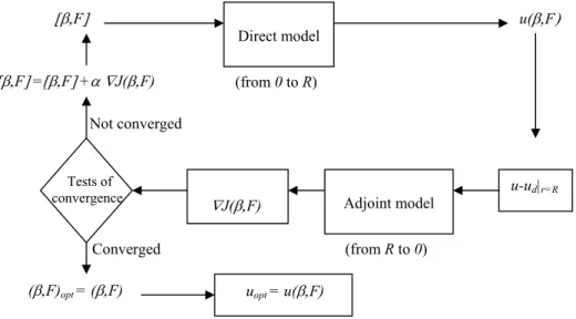
. The global optimization procedure is summarized in Fig. 1. In order to accelerate the convergence, we use a classical conjugate gradient method of Polack-Ribière type rather than the simplest method of steepest descent. The algorithm that is used is described in [21] and proceeds in two steps. First, the direction of minimization is computed following the Polack-Ribière algorithm that exploits the gradient of the cost function Eq.(20). Then the step length along the minimization direction is computed thanks to a soft linesearch algorithm that applies the Wolfe criteria. The interested reader is referred to [21] for a precise description of the implemented algorithm.Figure 1. Optimization algorithm – J is minimized until some convergence criteria are attained.
[β,F] =[β,F] +α ∇J(β,F) [β,F] Direct model (from 0 to R) u(β,F) u-ud|r=R Adjoint model (from R to 0) ∇J(β,F) Tests of convergence (β,F)opt = (β,F) uopt = u(β,F) Not converged Converged
3 Numerical results
The numerical results that are presented in this section rely on the finite-difference implementation of the direct and the adjoint models presented above, and of the associated discrete version of the gradient of the cost function. Before applying the inversion procedure, a gradient check (not shown here) was performed.
For a frequency of 500 Hz, we present the results obtained with an isovelocity sound speed profile in the water column of 1500 m s-1. The true non local impedance boundary
conditions were initially calculated for a sandy reflecting bottom with a compression speed of 1600 m s-1, an attenuation of 0.5 dB/λ and a density of 1.8 g cm-3. The initial
ones were obtained with a soft sediment (mud) characterized by a compression speed of 1505 m s-1, the other parameters remaining unchanged. No more than 5 or 6 iterations of
the optimization algorithm were needed for the algorithm to converge. However, due to the drastic convergence criteria we adopted for our calculations, we reached a maximum of 10 iterations. The corresponding computations, performed on a high-end PC (Pentium IV, 2 GHz), required around 20 minutes for a complete inversion. By optimizing the convergence criteria, this could be reduced by a factor of two.
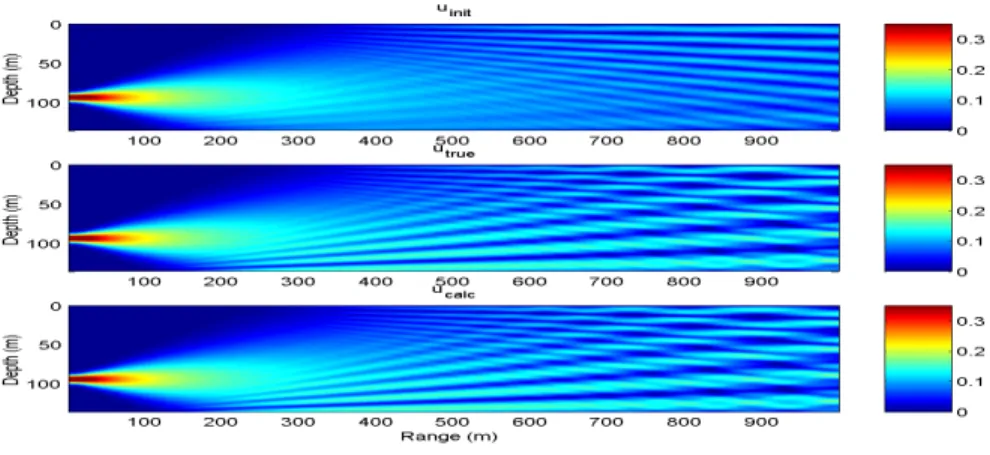
Figure 2 gives an overall representation of the reconstruction of the field in the entire range-depth domain. Although the initial field (top) was quite different from the true field (middle), the field calculated after inversion (bottom) agrees very well with the true one. The improvement of the acoustic pressure filed is drastic, the initial error for ranges greater than 400 m being reduced from 30-40% to only 2% approximately.
Figure 2. Visualization of the amplitude of the initial (top), true (middle) and inverted (bottom) u fields for
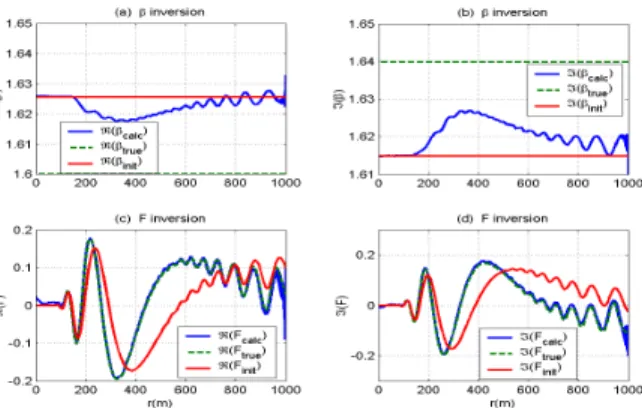
Figure 3. Comparison of the initial, the true and the inverted control parameters – (a)(b) Inversion of the real and imaginary parts of the β parameter – (c)(d) Inversion of the real and imaginary parts of the F parameter.
Figure 3 is devoted to the representation of the control parameters. We can observe that the accuracy of the
F
parameter is excellent after the inversion process. On the contrary, theβ
parameter is badly determined, which is certainly due to the ill-posednature of the inverse problem. The use of a wider angle PE approximation is susceptible to improve our results since the angular limitation of the standard PE approximation imposes that the chosen Gaussian source has no interaction with the bottom near the source. This assumption is under investigation.
4 Conclusions
We have generalized the variational approach that was presented in [14]. Here we treat the case of a PE propagation model constrained by NLBC's to simulate realistic environments in underwater acoustics. The obtained results are promising. They show that for a reasonable computational cost punctual acoustical data can be assimilated (here, vertical array data) which results in a global and drastic improvement of the prediction of complex pressure fields. The other central concept underlying our variational approach is that of the acoustically equivalent medium. This results in a rather abstract but concise representation of the geoacoustic properties of the seabed via its non local boundary conditions. These NLBC's are not easily related to the classical geoacoustic parameters of the bottom but are able to simulate the same acoustical behavior, at least for the simple but realistic environments considered in our simulations. In sonar applications, one of the main objectives is to be able to predict the acoustical losses in the water column. For this purpose the concept of acoustically equivalent medium is relevant and NLBC's are therefore good potential candidates as equivalent models. The presented method is rather new and should be studied in order to improve the generality of the approach. Further works should be involved in the use of sparse linear arrays and wider angle PE approximations or other propagation models. The application of the method will also be studied in the case of more complex seabed properties (multi-layered sub-bottoms). More importantly, and following the last tendencies in geoacoustic inversion, multi-tone and broadband signals will be considered in order to physically constrain the inverse problem and to aim at a unique inverted solution.
References
1. Chapman R., Tolstoy A., Benchmarking geoacoustic inversion methods - Special Issue, J. Comp. Acoust.
6, N°1&2 (1998) 289 pages.
2. Hermand J.-P., Broad-band geoacoustic inversion in shallow water from waveguide impulse response measurements on a single hydrophone: Theory and experimental results, IEEE J.Ocean.Eng. 24(1) (1999) pp. 41-66.
3. Lions J.-L., Contrôle optimal des systèmes gouvernés par des équations aux dérivées partielles (Dunod, Paris, 1968). In French.
4. Lions J.-L., Contrôlabilité exacte, perturbations et stabilisation des systèmes distribués, Vol. 1 (Masson, Paris, 1988). In French.
5. Talagrand O., Courtier P., Variational assimilation of meteorological observations with the adjoint vorticity equation - Part I, Quaterly J. Royal Meteo. Soc. 113 (1987) pp. 1311-1328.
6. Courtier P., Talagrand O., Variational assimilation of meteorological observations with the adjoint vorticity equation - Part II, Quaterly J. Royal Meteo. Soc. 113 (1987) pp.1329-1347.
7. Leredde Y., Lellouche J-M., Devenon J-L., Dekeyser I., On initial boundary conditions and viscosity coefficient control for Burgers' equation, Int. J. Num. Meth. Fluids 28 (1998) pp.113-128.
8. Schröter J., Variational assimilation of GEOSAT data into an eddy-resolving model of the Gulf-Stream extension area, J. Geophys. Ocean. 23 (1992) pp.925-953.
9. Plessix R-E., De Roeck Y-H., Chavent G., Waveform inversion of reflection seismic data for kinematic parameters by local optimization, SIAM J. Scient. Comp. 20 (1999) pp. 1033-1052.
10. Jameson A., Aerodynamic design via control theory, J. Scient. Computing, 3 (1988) pp.233-260.
11. Le Dimet F.X., Talagrand O., Variational algorithms for analysis and assimilation of meteorological observation: Theoretical aspects, Tellus 38 (1985) pp.309-322.
12. Belmiloudi A., Brossier F., A control method for assimilation of surface data in a linearized Navier-Stokes-type problem related to oceanography, SIAM J. Control. Optim. 35 (1997) pp.2183-2197.
13. Cacucci D., Sensitivity theory for nonlinear systems. Part I: Non linear functional analysis approach, J.
Math. Physics 22 (1981) pp.2794-2812.
14. Asch M., Le Gac J-C., Helluy P., An adjoint method for geoacoustic inversion, Invited Lecture, In Proc.
PICOF’02 2nd Conference on Inverse Problems, Control and Shape Optimization, Carthage, Tunisia
(2002).
15. Hursky P., Porter M., Cornuelle B.D., Hodgkiss W.S., Kuperman W.A., Adjoint-assisted inversion for shallow water environment parameters, In Impact of Littoral Environmental Variability on Acoustic
Predictions and Sonar Performance, eds. N.G. Pace and F.B. Jensen, Kluwer Academic Publishers (2002)
pp. 449-456.
16. Robertson J.S., Siegmann W.L., Jacobson M., Low frequency sound propagation modeling over a locally reacting boundary with the parabolic approximation, J. Acoust. Soc. Am. 98(2) (1995) pp.1130-1137.
17. Jensen F.B., Kuperman W.A., Porter M.B., Schmidt H., Computational Ocean Acoustics (AIP Series in Modern Acoustics and Signal Processing, New York, 1994)
18. Papadakis J.S., Impedance formulation of the bottom boundary condition for the parabolic equation model in underwater acoustics, in J.A. Davis, D. White and R.C. Cavanagh, "NORDA parabolic equation
workshop, 31 march - 3 April 1981", Tech. Note 143, Naval Ocean Research and Development Activity, NSTL Station, MS, 1982, available from NTIS, No.. AD-121 932 (1981) p.83.
19. Yevick D., Thomson D.J., Non local boundary conditions for finite difference parabolic equation solvers,
J. Acoust. Soc. Am. 106(1) (1999) pp.143-150.
20. Tappert F.D., The parabolic approximation method, in Wave Propagation in Underwater Acoustics, eds.
J.B. Keller and J.S. Papadakis, (Spinger-Verlag, New-York,1977) pp.224-287.
21. Frandsen P.E., Jonasson K., Nielsen H.B., Tingleff O., Unconstrained optimization, Lecture Note, IMM-LEC-2, Technical University of Denmark (1999). Online version available at the site <http://www.imm.dtu.dk/~hbn/software.html>.
22. Asch M., Le Gac J-C., Adjoint modeling for geoacoustic inversion - I: PE approximation with local impedance boundary conditions, Submitted to J. Acoust. Soc. Am. (July 2003).
23. Le Gac J-C., Asch M., Adjoint modeling for geoacoustic inversion - II: PE approximation with non local impedance boundary conditions, Submitted to J. Acoust. Soc. Am. (July 2003).