HAL Id: hal-00304111
https://hal.archives-ouvertes.fr/hal-00304111
Submitted on 17 Apr 2008HAL is a multi-disciplinary open access
archive for the deposit and dissemination of sci-entific research documents, whether they are pub-lished or not. The documents may come from teaching and research institutions in France or abroad, or from public or private research centers.
L’archive ouverte pluridisciplinaire HAL, est destinée au dépôt et à la diffusion de documents scientifiques de niveau recherche, publiés ou non, émanant des établissements d’enseignement et de recherche français ou étrangers, des laboratoires publics ou privés.
Twelve years of global observation of formaldehyde in
the troposphere using GOME and SCIAMACHY sensors
I. de Smedt, J.-F. Müller, T. Stavrakou, R. van der A, H. Eskes, M. van
Roozendael
To cite this version:
I. de Smedt, J.-F. Müller, T. Stavrakou, R. van der A, H. Eskes, et al.. Twelve years of global observation of formaldehyde in the troposphere using GOME and SCIAMACHY sensors. Atmospheric Chemistry and Physics Discussions, European Geosciences Union, 2008, 8 (2), pp.7555-7608. �hal-00304111�
ACPD
8, 7555–7608, 2008 Formaldehyde observation by GOME and SCIAMACHY I. De Smedt et al. Title Page Abstract Introduction Conclusions References Tables Figures ◭ ◮ ◭ ◮ Back CloseFull Screen / Esc
Printer-friendly Version
Interactive Discussion
Atmos. Chem. Phys. Discuss., 8, 7555–7608, 2008 www.atmos-chem-phys-discuss.net/8/7555/2008/ © Author(s) 2008. This work is distributed under the Creative Commons Attribution 3.0 License.
Atmospheric Chemistry and Physics Discussions
Twelve years of global observation of
formaldehyde in the troposphere using
GOME and SCIAMACHY sensors
I. De Smedt1, J.-F. M ¨uller1, T. Stavrakou1, R. van der A2, H. Eskes2, and M. Van Roozendael1
1
Belgian Institute for Space Aeronomy (BIRA-IASB), Avenue Circulaire, 3, 1180, Brussels, Belgium
2
Royal Netherlands Meteorological Institute (KNMI), Wilhelminalaan 10, 3732 GK, De Bilt, The Netherlands
Received: 18 February 2008 – Accepted: 26 March 2008 – Published: 17 April 2008 Correspondence to: I. De Smedt ([email protected])
ACPD
8, 7555–7608, 2008 Formaldehyde observation by GOME and SCIAMACHY I. De Smedt et al. Title Page Abstract Introduction Conclusions References Tables Figures ◭ ◮ ◭ ◮ Back CloseFull Screen / Esc
Printer-friendly Version
Interactive Discussion Abstract
This work presents global tropospheric formaldehyde columns retrieved from near-UV radiance measurements performed by the GOME instrument onboard ERS-2 since 1995, and by SCIAMACHY, in operation on ENVISAT since the end of 2002. A special effort has been made to ensure the coherence and quality of the CH2O dataset
cover-5
ing the period 1996–2007. Optimised DOAS settings are proposed in order to reduce the impact of two important sources of error in the derivation of slant columns, namely, the polarisation anomaly affecting the SCIAMACHY spectra around 350 nm, and a ma-jor absorption band of the O4 collision complex centred near 360 nm. The air mass
factors are determined from scattering weights generated using radiative transfer
cal-10
culation taking into account the cloud fraction, the cloud height and the ground albedo. Vertical profile shapes of CH2O are provided by the global CTM IMAGES based on an
up-to-date representation of emissions, atmospheric transport and photochemistry. A comprehensive error analysis is presented. This includes errors on the slant columns retrieval and errors on the air mass factors which are mainly due to uncertainties in
15
the a priori profile and in the cloud properties. The major features of the retrieved formaldehyde column distribution are discussed and compared with previous CH2O datasets over the major emission regions.
1 Introduction
Despite its short lifetime, formaldehyde (CH2O) is one of the most abundant
hydrocar-20
bons in the atmosphere and plays a central role in tropospheric chemistry, as an im-portant indicator of non-methane volatile organic compound (NMVOC) emissions and photochemical activity. CH2O is a primary emission product from biomass burning and from fossil fuel combustion, but its principal source in the atmosphere is the photochem-ical oxidation of methane and non-methane hydrocarbons. Besides dry and wet
depo-25
ACPD
8, 7555–7608, 2008 Formaldehyde observation by GOME and SCIAMACHY I. De Smedt et al. Title Page Abstract Introduction Conclusions References Tables Figures ◭ ◮ ◭ ◮ Back CloseFull Screen / Esc
Printer-friendly Version
Interactive Discussion
CO+H2and CO+2HO2) and oxidation by OH radicals (yielding CO+HO2+H2O).
Glob-ally, the methane oxidation represents the main CH2O source, accounting for more
than half the global CH2O production, the remainder being produced by NMVOC
oxi-dation (Stavrakou et al., 20081). Over the continents, however, due to its short lifetime, formaldehyde is a good indicator for the emissions of short-lived NMVOCs, like
iso-5
prene and the pyrogenic NMVOCs. Therefore, satellite measurements of CH2O can
be used to constrain NMVOC emissions in current state-of-the-art chemical transport models (Abbot et al., 2003; Palmer et al., 2006; Fu et al., 2007; Shim et al., 2005).
The CH2O data presented in this study are derived from observations made by the
GOME and SCIAMACHY instruments. Previous retrievals of formaldehyde have been
10
obtained from GOME measurements by application of the Differential Optical Absorp-tion Spectroscopy (DOAS) method, using three absorpAbsorp-tion bands of CH2O between
337 and 359 nm (Thomas et al., 1998; Chance et al., 2000; Wittrock et al., 2000; Mar-bach et al., 2004; De Smedt et al., 2006). These studies demonstrated the usefulness of satellite observations of CH2O columns as a mean to provide constraints on the
15
emissions of NMVOCs. For example, GOME CH2O columns have been used to
de-rive the seasonal and interannual variability of isoprene emissions over North America (Palmer et al., 2003; Abbot et al., 2003; Palmer et al., 2006), over Southeast Asia (Fu et al., 2007) and on the global scale (Shim et al., 2005). Despite SCIAMACHY provides nadir UV-visible radiance measurements suitable to complement GOME observations,
20
until now, only one study reports its use to retrieve CH2O columns (Wittrock et al.,
2006). This is mainly due to the existence of a strong polarisation anomaly affecting the SCIAMACHY spectra around 350 nm, preventing the straightforward application of the CH2O retrieval settings derived from GOME. One way to sidestep this problem
is to fit CH2O at shorter UV wavelengths, hence avoiding the unwanted polarisation
25
1
Stavrakou, T., M ¨uller, J.-F., De Smedt, I., van Roozendael, M., van der Werf, G., Giglio, L., and Guenther, A.: Evaluating the performance of pyrogenic and biogenic emission inventories against one decade of space-based formaldehyde columns, J. Geophys. Res, in preparation, 2008.
ACPD
8, 7555–7608, 2008 Formaldehyde observation by GOME and SCIAMACHY I. De Smedt et al. Title Page Abstract Introduction Conclusions References Tables Figures ◭ ◮ ◭ ◮ Back CloseFull Screen / Esc
Printer-friendly Version
Interactive Discussion
signature. In this paper, we propose a new fitting window applicable to both SCIA-MACHY and GOME, and we use it to generate a 12-years long data set of CH2O
columns that consistently combines the two instruments. This CH2O product has
been developed in the framework of the TEMIS (http://www.temis.nl) and PROMOTE (http://www.gse-promote.org) projects and is available on their websites. After a brief
5
description of the satellite instruments in Sect. 2, Sect. 3 presents the retrieval method, more specifically, the slant column fitting and the determination of the air mass factors. Section 4 provides a detailed description of the error budget and of the averaging ker-nels. Section 5 presents the global distribution and temporal evolution of the CH2O
vertical columns derived in this study, as well as a discussion of differences with
previ-10
ously retrieved datasets.
2 GOME and SCIAMACHY spectrometers
GOME (onboard the ERS-2 satellite launched in April 1995) and SCIAMACHY (on-board the ENVISAT satellite launched in March 2002) are absorption spectrometers measuring the Earth backscattered sunlight as well as the direct solar irradiance
spec-15
trum. Both instruments fly on polar sun-synchronous orbits. GOME measures in a wavelength range covering the UV, visible and near-infrared from 240 nm up to 790 nm, at the moderate resolution of 0.15 to 0.4 nm. It crosses the equator at 10:30 h lo-cal time. The full width of a normal GOME scanning swath is 960 km, divided into three ground pixels. The scan measures 40 km in the direction of flight. Global
cov-20
erage is obtained in three days at the equator (Burrows et al., 1999b). GOME has been recording spectra with global coverage until June 2003. It is still in operation but with limited Earth coverage over the Northern Hemisphere and part of Antarctica. The spectra of SCIAMACHY are recorded between 240 and 1700 nm and in selected regions of the short wave infrared between 1900 and 2400 nm (resolution between
25
0.2 nm and 1.5 nm). SCIAMACHY has three different viewing geometries: nadir, limb, and sun/moon occultation. In its nadir view, the SCIAMACHY swath width is
equiva-ACPD
8, 7555–7608, 2008 Formaldehyde observation by GOME and SCIAMACHY I. De Smedt et al. Title Page Abstract Introduction Conclusions References Tables Figures ◭ ◮ ◭ ◮ Back CloseFull Screen / Esc
Printer-friendly Version
Interactive Discussion
lent to GOME, but it is divided into 14 ground pixels of 60 km over 30 km. The ground resolution is therefore seven times higher than in the case of GOME but with an equiv-alently lower signal to noise ratio due to the shorter integration time. As a consequence of the alternating nadir and limb views, global coverage is only achieved in six days. The crossing time at the equator is 10:00 h local time (Bovensmann et al., 1999).
5
Both instruments have demonstrated their capability to observe atmospheric trace gas species like O3, NO2, BrO, SO2, OClO and CH2O (Eisinger et al., 1998; Richter et al., 1998; Chance et al., 2000; Richter and Burrows, 2002; Boersma et al., 2004; K ¨uhl et al., 2004; Martin et al., 2004; Liu et al., 2005; Khokhar et al., 2005; Richter et al., 2005) and also, in the case of SCIAMACHY, infrared greenhouse gases like CH4, CO and
10
CO2(Frankenberg et al., 2005; Buchwitz et al., 2005).
3 Retrieval method
Owing to the sharp absorption bands of CH2O in the UV, the differential optical ab-sorption spectroscopy technique (DOAS) (Platt, 1994) can be used to derive CH2O
from satellite observations. This method consists of two independent steps. Firstly,
15
the species concentration integrated along the viewing path of the satellite, also called slant column density, is derived from the satellite radiance using the Beer-Lambert the-ory in the atmosphere. Secondly, the slant column is converted into a vertical column through the determination of an air mass factor (AMF) defined as the ratio between calculated slant and vertical columns. In the troposphere, the AMF cannot be simply
20
derived from geometrical considerations accounting for the solar and viewing angles of the observation. Multiple scattering due to air molecules, aerosols and clouds, com-bined with surface albedo effects, modifies the vertical distribution of the effective light path, so that the total vertically averaged AMF is a function of the vertical distribution of the absorber, which therefore has to be known a priori.
ACPD
8, 7555–7608, 2008 Formaldehyde observation by GOME and SCIAMACHY I. De Smedt et al. Title Page Abstract Introduction Conclusions References Tables Figures ◭ ◮ ◭ ◮ Back CloseFull Screen / Esc
Printer-friendly Version
Interactive Discussion
3.1 Slant column retrieval
Assuming an optically thin atmosphere, the various paths of the scattered photons can be represented by one effective photon path length averaged over the fitting interval. The Beer-Lambert law can then be expressed as follows, separating the broadband contributions (Rayleigh and Mie scattering) from the sharp spectral signatures due to
5 molecular absorption: I(λ) =µ0 π .I0(λ). exp " − X i Ns i.σi(λ) − X p ap.λp # . (1)
In this expression, I and I0are the measured earthshine radiance and solar irradiance
spectra, respectively, and µ0is the cosine of the solar zenith angle. Ns
i and σi are re-spectively the slant column and the absorption cross section of each molecule and ap
10
are the coefficients of the polynomial function of order p accounting for terms varying slowly with the wavelength. The product Ns
i·σi is called the optical density of the ith molecule. The DOAS fit consists in expressing the optical density as a function of the logarithm of the ratio of the measured intensities. The column densities are deduced by solving the resulting system of linear equations (e.g. Platt, 1994). In practice,
ad-15
ditional non-linear effects have to be taken into account like for example, wavelength shifts between I and I0due to the Doppler effect or induced by thermal instabilities in
the instrument, or the eventual contamination of measured radiances by spectral stray-light, which requires the introduction of an intensity offset parameter. The Ring effect (Grainger et Ring, 1962), which arises due to inelastic scattering processes (Vountas
20
et al., 1998), has a strong impact on spectroscopic measurements using the DOAS method, particularly for minor absorbers whose weak absorption features can be com-pletely masked by its structures. In DOAS, the Ring effect is usually accounted for by means of a pseudo absorber also included in the fit (Chance and Spurr, 1997).
Despite the relatively large abundance of CH2O in the atmosphere (on the order
25
ACPD
8, 7555–7608, 2008 Formaldehyde observation by GOME and SCIAMACHY I. De Smedt et al. Title Page Abstract Introduction Conclusions References Tables Figures ◭ ◮ ◭ ◮ Back CloseFull Screen / Esc
Printer-friendly Version
Interactive Discussion
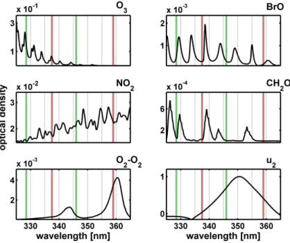
columns in earthshine radiances is a challenge because of the low optical density of CH2O compared to other UV absorbers. As displayed in Fig. 1, the typical CH2O optical density is about 2.5 times smaller than for BrO and up to 50 times smaller than for NO2. Therefore, the detection of CH2O is limited by the signal to noise ratio of
the measured radiance and by possible spectral interferences due to other molecules
5
absorbing in the same fitting interval, mainly ozone. In this work, most DOAS settings are common to both GOME and SCIAMACHY retrievals. The CH2O absorption cross
sections used in the DOAS fit are those of Cantrell et al. (1990), convolved to the resolution of the instrument. The fitting procedure includes reference spectra for other interfering species (O3, NO2, BrO, OClO and the O2–O2 (or O4) collision complex).
10
The Ring effect is corrected according to Chance and Spurr (1997). A linear intensity offset correction is further applied as well as a polynomial closure term of order 5. In order to minimise the impact of the GOME diffuser plate related artefact (Richter and Wagner, 2001) and to minimize fitting residuals, daily radiance spectra are used as the
I0reference. These are selected in a region of the equatorial Pacific Ocean where the
15
formaldehyde column is assumed to be low and stable in time (Stavrakou et al., 20081). Taking into account the spectral and instrumental constraints, the fitting window has been chosen in order to (1) maximize the sensitivity to formaldehyde, (2) minimize the fitting residuals and the dispersion of the retrieved CH2O slant columns and (3)
mini-mize the interferences with other absorbers. From inspection of the CH2O absorption
20
cross sections in Fig. 1, it can be seen that a maximum of five characteristic absorption bands are available in the spectral interval from 325 to 360 nm. A compromise has to be found when defining the DOAS settings, since the fitting accuracy is limited at the shorter wavelengths by the increased O3absorption and the resulting interference
with the formaldehyde fit, and at longer wavelengths by the interference with the
SCIA-25
MACHY polarisation feature around 350 nm (Fig. 1). Several fitting intervals have been tested as to their ability to produce consistent and stable retrievals from both GOME and SCIAMACHY. The best compromise, which maximizes the number of CH2O
ACPD
8, 7555–7608, 2008 Formaldehyde observation by GOME and SCIAMACHY I. De Smedt et al. Title Page Abstract Introduction Conclusions References Tables Figures ◭ ◮ ◭ ◮ Back CloseFull Screen / Esc
Printer-friendly Version
Interactive Discussion
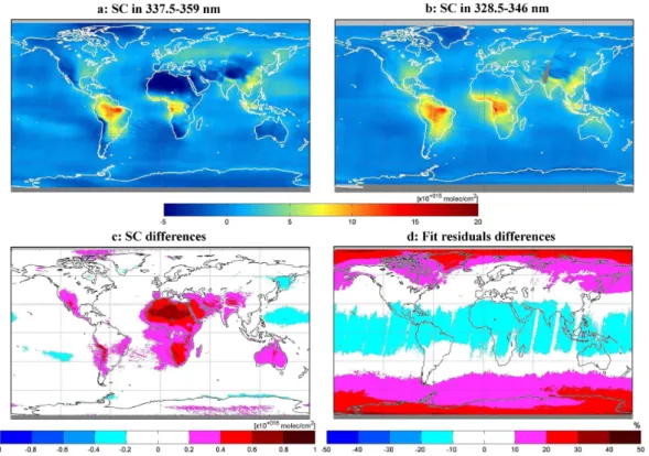
peak around 350 nm, was found to lie in the 328.5–346 nm wavelength region. De-spite the stronger interference with O3absorption at these wavelengths, the use of the 328.5–346 nm window improves the GOME slant columns compared to retrievals com-monly performed in the 337.5–359 nm region. Previous studies using this later window exhibited anomalous features like for example, excessively low (sometimes negative)
5
columns above desert regions like Sahara and Australia (Wittrock et al., 2000; De Smedt et al., 2006), or systematic structures above oceans in apparent contradiction with tropospheric models (Abbot et al., 2003; Palmer et al., 2006). The use of the newly proposed 328.5–346 nm interval leads to a reduction of the noise over oceans and brings the slant column values above desert regions at the level of the background
10
(Fig. 2a and b). The CH2O values retrieved using the two fitting windows are gener-ally consistent within 2·1015molec./cm2, in particular above regions of enhanced emis-sions. The biggest differences are found above desert regions, mainly in Africa, the Middle East and Australia, where they range between 2·1015 and 10·1015molec./cm2. Fitting residuals are lower by 15% in the Tropics, but they increase more rapidly with
15
solar zenith angle and exceed the fitting residuals of the 337.5–359 nm window pole-ward of 50◦ because of a stronger interference with O
3 (Fig. 2c and d). Fitting tests
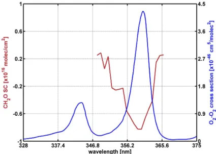
have been performed, showing that the slant column underestimation above desert regions is not observed as long as the upper limit of the fitting window is kept under 350 nm. Furthermore, the magnitude of the negative bias above Sahara, represented
20
as a function of the upper limit chosen for the fitting window (Fig. 3), correlates well with the O4absorption band peaking at 360 nm. This suggests that the low CH2O columns
observed above deserts are most likely due to an O4-related fitting artefact rather than
a real particularity of the formaldehyde distribution. Desert regions are generally cloud-free and therefore, they correspond to the highest O4columns observed globally. The
25
known uncertainties of the O4 cross sections are expected to significantly impact the
quality of the CH2O retrievals in these regions, especially when the strong absorption band of O4at 360 nm is included in the fit, even partially.
ACPD
8, 7555–7608, 2008 Formaldehyde observation by GOME and SCIAMACHY I. De Smedt et al. Title Page Abstract Introduction Conclusions References Tables Figures ◭ ◮ ◭ ◮ Back CloseFull Screen / Esc
Printer-friendly Version
Interactive Discussion
SCIAMACHY CH2O columns are found to be consistent with GOME ones when re-trieved in the same window. Among other fitting windows tested for SCIAMACHY, the 328.5–346 nm interval displays the lowest differences with GOME, as verified over the six first months of 2003, when the two satellite measurements globally overlap. This wavelength interval also provides the lowest dispersion in the SCIAMACHY results.
5
Examples of CH2O optical density fits are shown in Fig. 4 for a GOME pixel in
Septem-ber 1997 and a SCIAMACHY pixel in SeptemSeptem-ber 2006, both located over Indonesia during fire episodes. The SCIAMACHY CH2O retrieval is noisier as a result of the
smaller pixel sizes (about a factor of 7 compared to GOME). The standard deviation in the SCIAMACHY columns is 2.4 higher that in the case of GOME, slightly less than
10
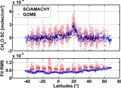
the value expected from photon statistical consideration (√7=2.65). This shows that the noise in the retrieved columns is consistent with the signal to noise ratio of the instruments. Figure 5 shows the slant columns for two overlapping orbits of GOME and SCIAMACHY over Eastern China, on the 14th of April 2003. The mean CH2O val-ues agree very well but, in this case, the standard deviation in the SCIAMACHY slant
15
columns only exceeds GOME one by 30%, as a result of the long term degradation of the GOME instrument from 1996 until 2003 (see Sect. 4.1).
3.2 Reference sector correction
Because a daily radiance spectrum is used as control spectrum for the DOAS fit, the retrieved slant columns actually represent the difference in slant column with respect
20
to the slant column contained in the control spectrum. Hence the quantity of formalde-hyde present in the reference spectrum must be estimated on a daily basis, based on suitable external information. Furthermore, an analysis of the raw slant column mea-surements reveals obvious zonally and seasonally dependent artefacts. Indeed, over the remote Pacific Ocean, the formaldehyde columns are often found to differ from
25
the background levels attributed to methane oxidation by more than 1·1016molec./cm2. This is especially clear at latitudes higher than 60◦ and in March. This behaviour is
ACPD
8, 7555–7608, 2008 Formaldehyde observation by GOME and SCIAMACHY I. De Smedt et al. Title Page Abstract Introduction Conclusions References Tables Figures ◭ ◮ ◭ ◮ Back CloseFull Screen / Esc
Printer-friendly Version
Interactive Discussion
are very important at high solar zenith angles in spring. Fortunately, these interferences are small in regions where the sources of formaldehyde are significant. However, to reduce the impact of these artefacts, an absolute normalisation is applied on a daily basis using the reference sector method (Khokhar et al., 2005). The reference sector is chosen in the central Pacific Ocean (140–160◦W), where the only significant source
5
of CH2O is the CH4oxidation. The latitudinal dependency of the CH2O slant columns
in the reference sector is modelled by a polynomial, subtracted from the slant columns and replaced by the CH2O background taken from the tropospheric 3-D-CTM IMAGES (M ¨uller and Stavrakou, 2005) in the same region. A similar normalisation approach has been applied in previous studies (e.g. Abbot et al., 2003).
10
3.3 Air mass factors determination
The next step in the retrieval of tropospheric CH2O total columns is the calculation of the air mass factors necessary to convert slant columns into corresponding vertical columns. As already mentioned, the AMF is defined by the ratio of the slant column to the vertical column. In the troposphere, scattering by air molecules and variable
15
amounts of clouds and aerosols reduces the penetration of the UV radiation leading to complex altitude-dependent enhancement factors. As a result, the column-averaged AMF is sensitive to the vertical distribution of the absorbing molecule as well as to other factors controlling the penetration and reflection of the UV photons on their way through the atmosphere. Full multiple scattering calculations are therefore required
20
for its determination. Nevertheless, in the case of weak absorbers like CH2O, the calculation can be simplified by introducing the concept of scattering weights which are independent of the trace gas concentration profile (Palmer et al., 2001). The total column air mass factor can be obtained from the formula:
M = Z
atm
W(z, µ0, µ, Cf, Ch, as, hs).S(z, lat, long, month).d z, (2)
ACPD
8, 7555–7608, 2008 Formaldehyde observation by GOME and SCIAMACHY I. De Smedt et al. Title Page Abstract Introduction Conclusions References Tables Figures ◭ ◮ ◭ ◮ Back CloseFull Screen / Esc
Printer-friendly Version
Interactive Discussion
where the scattering weight W represents the sensitivity of the satellite measurements to the molecule concentration in function of the altitude z. W depends only on the observation geometry (µ0and µ are the cosine of the solar and viewing zenith angles
respectively) and on the scattering properties of the atmosphere, the cloud fraction and cloud height (Cf and Ch), the surface albedo (as) and the surface altitude (hs). In this
5
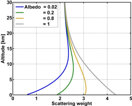
work, scattering weights have been evaluated from radiative transfer calculations per-formed with a pseudo-spherical version of the DISORT code (Kylling et al., 1995). The scattering properties of the atmosphere have been modelled at 340 nm for a number of representative viewing geometries, surface albedos and ground altitudes, and stored in a look-up table. In Fig. 6, the scattering weight is represented as a function of the
10
altitude for different values of the albedo. As can be seen, the sensitivity of the satel-lite measurement decreases towards the surface due to increased scattering efficiency and corresponding reduction of the photon path penetration. In contrast, the sensitivity increases at higher albedo because more light is then reflected towards the satellite. A cloud correction is applied based on the independent pixel approximation (Martin et
15
al., 2001). Accordingly, the scattering weight of a partly cloudy pixel is a combination of its cloud free part and its fully cloudy part. A normalisation by the reflectivities of the cloudy and cloud free parts of the pixel (Rclearand Rcloud) is included:
W =(1 − Cf).Wclear(a ground s , hs).Rclear+ Cf.Wcloud(a cloud s , Ch).Rcloud (1 − Cf).Rclear+ Cf.Rcloud . (3)
The cloud fraction, cloud height and cloud albedo (aclouds ) are obtained from the
20
FRESCO v5 cloud product (Koelemeijer et al., 2002) as delivered on the TEMIS project website (http://www.temis.nl). The distribution of surface albedo is taken from the clima-tology of Koelemeijer et al. (2003), which provides monthly Lambert-equivalent reflec-tivity at 335 nm. No explicit correction is applied for aerosols, but their impact is partially accounted for by the cloud correction scheme, as further explained in Sect. 4.3.
25
In Eq. (2), the shape factor S represents the normalised profile of the absorbing molecule. In this study, the monthly output of an updated version of the IMAGES
ACPD
8, 7555–7608, 2008 Formaldehyde observation by GOME and SCIAMACHY I. De Smedt et al. Title Page Abstract Introduction Conclusions References Tables Figures ◭ ◮ ◭ ◮ Back CloseFull Screen / Esc
Printer-friendly Version
Interactive Discussion
chemical transport model (M ¨uller and Stavrakou, 2005) has been used to specify the vertical profile of the CH2O distribution. IMAGESv2 provides the global distribution of
68 chemical compounds at a resolution of 5◦with 40 vertical sigma-pressure levels
be-tween the surface and the pressure of 45 hPa. The chemical mechanism of the model has been optimized with respect to CH2O production from isoprene and from pyrogenic
5
NMVOCs based on a detailed box model study using the Master Chemical Mechanism (MCM, Saunders et al., 2003) and an updated speciation profile of pyrogenic emissions (Andreae and Merlet, 2001, Andreae, personal communication, 2007), as described in Stavrakou et al. (20081). The advection is driven by monthly wind fields from ECMWF analyses. The impact of wind variability at short timescales is represented using
hor-10
izontal diffusion coefficients estimated from the ECMWF wind variances. The param-eterization of convective transport uses the ERA40 updraft mass fluxes until 2001, and a climatological mean beyond this year. Anthropogenic emissions are taken from EDGAR v3.3 inventory for 1997 (Olivier et al., 2001). The biomass burning emissions are based on the GFEDv1 inventory, or alternatively the GFEDv2 inventory for burnt
15
biomass (van der Werf et al., 2004 and 2006). A diurnal cycle of biomass burning emissions based on Giglio (2007) is applied in the diurnal cycle calculations. Biogenic isoprene emissions are taken from the GEIA inventory (Guenther et al., 1995), or al-ternatively from an inventory based on the MEGAN emission model (Guenther et al., 2006) driven by ECMWF meteorological fields, as described in Muller et al. (2007).
20
Vertical CH2O profile shapes are provided on a monthly basis between 1997 and 2006
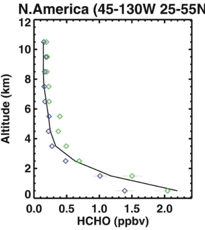
and interpolated for each satellite geolocation. The IMAGES profiles have been val-idated with various aircraft measurements like the INTEX-A campaign over Northern America in July–August 2004 (Singh et al., 2006). In Fig. 7, the IMAGESv2 profiles are compared with the mean observed vertical distribution during this campaign. The
mod-25
elled mixing ratios are in fairly good agreement with the measurements at all altitudes, although an overestimation is noted near the surface.
ACPD
8, 7555–7608, 2008 Formaldehyde observation by GOME and SCIAMACHY I. De Smedt et al. Title Page Abstract Introduction Conclusions References Tables Figures ◭ ◮ ◭ ◮ Back CloseFull Screen / Esc
Printer-friendly Version
Interactive Discussion
3.4 Tropospheric vertical columns
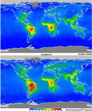
The global GOME CH2O vertical columns averaged over 7 years (from April 1996 to
December 2002) and the SCIAMACHY CH2O vertical columns averaged over the
fol-lowing 5 years (from January 2003 to December 2007) are displayed in Fig. 8. The level of agreement between the two datasets is very satisfactory. Both instruments capture
5
the regions of elevated NMVOC emission which are mainly located in the Tropics, in particular over Amazonia, Africa and Indonesia. The Eastern United States and South eastern Asia are also major regions of emission. The better resolution of SCIAMACHY allows observing more localized hotspots like for example the Highveld region in South Africa. In mid-latitude regions like Europe, Russia or Australia, SCIAMACHY columns
10
are generally higher than GOME ones by about 30%. The reason for this difference is currently unknown. In South America, the impact of the South Atlantic Anomaly is more pronounced in the SCIAMACHY columns.
4 Error analysis
A formulation of the error can be derived analytically starting from the equation of the
15
vertical column which directly results from the different steps detailed in Sect. 3:
Nv = (Ns− Ns0) M + N CT M v0 = ∆Ns M + N CT M v0 . (4)
In this expression, ∆Ns represents the difference between the fitted slant column Ns
and the mean slant column in the reference sector Ns0. N
CT M
v0 is the IMAGES
back-ground in the same region. M is the air mass factor. As these terms are determined
20
independently, the total error on the tropospheric vertical column can be expressed as (Boersma et al., 2004):
ACPD
8, 7555–7608, 2008 Formaldehyde observation by GOME and SCIAMACHY I. De Smedt et al. Title Page Abstract Introduction Conclusions References Tables Figures ◭ ◮ ◭ ◮ Back CloseFull Screen / Esc
Printer-friendly Version Interactive Discussion σN2 v = ( ∂Nv ∂Ns) 2.σ2 Ns+ ( ∂Nv ∂M) 2.σ2 M+ ( ∂Nv ∂Nv0) 2.σ2 Nv0CT M . (5)
In our case, it results from Eq. (4) that the total error can be derived from the following expression: σN2 v = 1 M2. σN2 srand N + 1 M2.σ 2 Nssyst + ( ∆Ns M2 ) 2.σ2 M + σ 2 Nv0CT M . (6) σN
srand and σNssyst are the random and systematic parts of the error on the slant
5
columns. The random error is reduced when the number of measurements increases. Therefore, in case of averaging, σNsrandcan be divided by the square root of the number
of satellite pixels taken into the mean (N). σM is the error on the air mass factor evalua-tion and σNv0CTM the error on the reference sector correction. Theses two latter sources of uncertainties have systematic but also random components that may average out
10
in space or in time. However, these components can hardly be separated in practice and we will consider these uncertainties as systematic. The total error calculated with Eq. (6) is therefore an upper limit of the real error on the vertical columns.
4.1 Error on slant columns
The random error on the slant column (σN
srand) can be expressed by the standard
de-15
viation of measured columns around the mean. Due to the degradation of the GOME instrument throughout the years and the resulting lower signal to noise ratio of the spectra, σN
srand has been found to increase from 4·10
15
molec./cm2 in 1996 up to 6·1015molec./cm2 in 2003. For SCIAMACHY, σNsrand reaches 1·10
16
molec./cm2 be-cause of the poorer signal to noise ratio associated to the shorter integration time of
20
this instrument. For single pixels, the random error on the slant columns is the most important source of error on the total vertical column. It can be reduced by averaging, but of course to the expense of a loss in time and/or spatial resolution.
ACPD
8, 7555–7608, 2008 Formaldehyde observation by GOME and SCIAMACHY I. De Smedt et al. Title Page Abstract Introduction Conclusions References Tables Figures ◭ ◮ ◭ ◮ Back CloseFull Screen / Esc
Printer-friendly Version
Interactive Discussion
The systematic errors on the slant columns are largely connected to uncertainties on the absorption cross sections included in the fit, although other sources of systematic errors also contribute to the error budget, like uncertainties related to instrumental effects (wavelength calibration, spectral stray light, slit function. . . ), or systematic misfit effects when for example, the absorption of the ozone molecule becomes so strong that
5
the DOAS approximation of an optically thin atmosphere is not fully satisfied anymore. Systematic slant column errors due to absorption cross section uncertainties and their correlations can be estimated using the Rodgers formalism (Rodgers et al., 2000) for a linear over-constrained problem like the DOAS inversion (Theys et al., 2007):
σN2 ssyst = m X j =1 Nsj2 hGSbjGTi. (7) 10
In this equation, the species index j (=1,. . . ,m) runs over all molecules taken into ac-count in the fit. G is the contribution matrix of the DOAS retrieval, constructed as
G =hKTKi−1KT where K (n×m, with n the number of wavelengths in the fitting
inter-val) is a matrix formed by the absorption cross sections. Nsjis the fitted slant column of the jth molecule and Sbj(n×n) is the cross section error covariance matrix. For CH2O,
15
the absorption cross section of Cantrell et al. (1990), recommended in the HITRAN database, has been used. This data set presents a resolution four times better in com-parison to the alternative data set of Meller and Moortgat (2000). Recently, however, the use of the Meller and Moortgat (2000) cross section has been recommended by Gratien et al. (2007) based on a study of the consistency between UV and infrared
20
absorption spectra of CH2O. We find that at GOME resolution and in the wavelength
range of interest for this study, the Cantrell et al. (1990) and the Meller and Moort-gat (2000) data sets differ by less than 12%, and we adopted this difference as an estimate of the systematic error on the CH2O differential cross section used in our
work. For the other absorbers included in the fit, only the random error on the cross
25
ACPD
8, 7555–7608, 2008 Formaldehyde observation by GOME and SCIAMACHY I. De Smedt et al. Title Page Abstract Introduction Conclusions References Tables Figures ◭ ◮ ◭ ◮ Back CloseFull Screen / Esc
Printer-friendly Version
Interactive Discussion
random uncertainties associated to the different absorption cross sections have been taken from the literature and are summarized in Table 1.
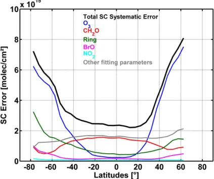
The total systematic error budget on the SCIAMACHY CH2O slant columns, resolved
into its various contributions, is represented in Fig. 9, for SCIAMACHY in March 2003. In the tropics, the uncertainty on the CH2O cross section contributes most, while at
5
higher latitudes, the uncertainties due to ozone absorption and the Ring effect dom-inate. Although this formalism accounts for correlation effects between the absorp-tion cross secabsorp-tions, it does not include sources of systematic error besides the cross section uncertainties. Therefore an additional contribution taken as 12% of the slant columns has been included to account for other sources of error. This 12% value has
10
been derived from retrieval tests, where the fitting windows (328.5–346 nm and 337.5– 359 nm), the calibration options (e.g. the type of the slit function), and the polynomial order for the stray light correction were varied respectively. As displayed in Fig. 9, the total error increases from 2.5·1015 molec./cm2 in the Tropics to 8·1015molec./cm2 at high latitudes. In the Tropics, fitting parameters like the retrieval window and the
15
CH2O absorption cross section are the most important sources of uncertainty. Ozone,
NO2 and BrO cross section errors have comparatively little impact in these regions. At higher latitudes, errors related to ozone absorption and the Ring effect are largely dominant, their contributions respectively reaching 7 and 3·1015molec./cm2. The error due to spectral interference with BrO absorption structures increases also at these
lat-20
itudes because, as for ozone, BrO is more abundant poleward. The contributions from the CH2O absorption cross section as well as other fitting parameters are relatively
constant meridianwise.
4.2 Error on the reference sector correction
The last term of Eq. (6) represents the uncertainty due to the reference sector
correc-25
tion. It has been evaluated as the monthly averaged differences between the IMAGES columns and the columns estimated using another tropospheric model, namely the TM model (Eskes et al., 2003a), above the reference sector from 1997 to 2002. The errors
ACPD
8, 7555–7608, 2008 Formaldehyde observation by GOME and SCIAMACHY I. De Smedt et al. Title Page Abstract Introduction Conclusions References Tables Figures ◭ ◮ ◭ ◮ Back CloseFull Screen / Esc
Printer-friendly Version
Interactive Discussion
range between 0.5 and 2·1015molec./cm2. Therefore, σNv0CTM is small compared to other error sources (see Fig. 12).
4.3 Error on the air mass factor
As explained in Sect. 3.3, the scattering properties of the atmosphere are represented using weighting functions that are calculated for different values of the solar and viewing
5
zenith angles, the surface albedo and the ground altitude. Cloud effects are treated according to the independent pixel approximation and the vertical distribution of CH2O is taken from the IMAGES model. Accordingly, the error on the column-averaged air mass factor depends on input parameters uncertainties and on the sensitivity of the air mass factor to each of them (Boersma et al., 2004):
10 σM2 = (∂M ∂as.σas) 2 + (∂C∂M f .σC f) 2 + (∂C∂M h .σC h) 2 + (∂M∂S.σS)2, (8)
where σas, σCf, σCh, σS represent respectively the uncertainties on the surface albedo, the cloud fraction, the cloud height and the profile shape, all taken from the literature or derived from comparisons with independent data, as summarized in Table 2. The errors on the solar angles, the viewing angles and the ground altitude are here supposed to
15
be negligible. The sensitivities, i.e., the air mass factor derivatives with respect to the different input parameters, have been evaluated for different representative conditions of observation and for different profile shapes. Figure 10a shows the air mass factor dependence on the ground albedo for two different formaldehyde profile shapes (in blue: profile typical of remote area, in red: typical of emission regions). The sensitivity,
20
i.e. the slope, is almost constant with albedo, being only slightly higher for low albedo values. As expected, the air mass factor sensitivity to albedo is found to be higher for an emission profile peaking near the surface than for a background profile more spread in altitude. As illustrated in Fig. 10b, the air mass factor sensitivity to the cloud fraction is significant only when the cloud lies below the CH2O layer. Indeed, for this figure,
25
ACPD
8, 7555–7608, 2008 Formaldehyde observation by GOME and SCIAMACHY I. De Smedt et al. Title Page Abstract Introduction Conclusions References Tables Figures ◭ ◮ ◭ ◮ Back CloseFull Screen / Esc
Printer-friendly Version
Interactive Discussion
case (in red) but below the main formaldehyde layer in the background case (in blue). Figure 10c shows the air mass factor variation with cloud altitude. The slope is large when the cloud height is located below or at the altitude of the formaldehyde peak. For higher clouds, the sensitivity of the air mass factor to any change in cloud altitude is very weak. In order to evaluate the impact of the uncertainty on the profile shape, we
5
have estimated the uncertainty on the peak altitude and its width, by comparisons of the model results with aircraft measurements performed during campaigns like INTEX-A above the United States in 2004 (Millet et al., 2006; Singh et al., 2006) or TRINTEX-ACE-INTEX-A in the Tropics in 1992 (Fishman et al., 1996; Emmons et al., 2000).
The contribution of each parameter to the total air mass factor error depends on the
10
observation conditions. Figure 11 displays the total error on the air mass factor as a function of the cloud fraction in two cases: when (a) the cloud height is at 8 km or (b) at 1 km. The contribution from each parameter to the total error is also displayed. For clear sky conditions, the total air mass factor error is estimated to be 18% with equal contributions from the albedo and the profile shape uncertainties. For a cloud fraction
15
of 0.5, the total error reaches 30% for a high cloud and 50% for a low cloud. The most important error sources are uncertainties on the cloud altitude and on the profile shape for low clouds (<2 km), particularly over emission regions. Other sources, like the albedo and the cloud fraction uncertainties represent smaller contributions to the total error on the air mass factor.
20
In this study, we have not explicitly considered the effect of aerosols on the air mass factors. To a large extent, however, the effect of the non-absorbing part of the aerosol extinction is implicitly included in the cloud correction (Boersma et al., 2004). Indeed, in the presence of aerosols, the cloud detection algorithm FRESCO is expected to overestimate the cloud fraction. Since non-absorbing aerosols and clouds have
sim-25
ilar effects on the radiation in the UV-visible range, the omission of aerosols is partly compensated by the overestimation of the cloud fraction, and the resulting error on air mass factor is small, typically below 16% (Boersma et al., 2004, Millet et al., 2006). In contrast, absorbing aerosols have a different effect on the air mass factors, since they
ACPD
8, 7555–7608, 2008 Formaldehyde observation by GOME and SCIAMACHY I. De Smedt et al. Title Page Abstract Introduction Conclusions References Tables Figures ◭ ◮ ◭ ◮ Back CloseFull Screen / Esc
Printer-friendly Version
Interactive Discussion
tend to decrease the sensitivity to CH2O concentration. In this case, the resulting error on the air mass factor can be as high as 30% (Palmer et al., 2001; Martin et al., 2003). This may, for example, affect significantly our derivation of CH2O columns in regions
dominated by biomass burning as well as over heavily industrialized regions.
4.4 Total error on the CH2O vertical column
5
From Eq. (6), the total error on the vertical column can be calculated for each satellite pixel. Figure 12 shows the total error on the monthly and zonally averaged vertical columns, as a function of latitude, calculated for March 2003. The number of SCIA-MACHY pixels involved in these averages being generally large, the contribution from slant column random errors is below 2%. Note that the total error is naturally much
10
larger when considering individual pixels. The error due to the reference sector correc-tion ranges from 5 to 12%. At low and mid latitudes, the contribucorrec-tions from the slant columns and from the air mass factor uncertainties are equivalent, with values between 10 and 20%. At higher latitudes, the error due to slant column uncertainties is larger (15–40%) mainly due to the typically larger ozone concentrations. The total error on
15
CH2O monthly means generally lies between 20 and 40% for both GOME and
SCIA-MACHY data. This estimation is in agreement with the value of 25–30% deduced by Millet et al. (2006) who compared air mass factors calculated with the GEOS–CHEM model and air mass factors derived from aircraft measurements over North America in summer 2004.
20
4.5 Averaging kernels
Averaging kernels (A) are commonly used to quantify how the retrieval process smoothes the actual vertical distribution of a measured quantity (see e.g. Rodgers, 2000). Column averaging kernels are particularly useful when comparing measured columns with e.g. model simulations, because they allow removing the effect of the
25
ACPD
8, 7555–7608, 2008 Formaldehyde observation by GOME and SCIAMACHY I. De Smedt et al. Title Page Abstract Introduction Conclusions References Tables Figures ◭ ◮ ◭ ◮ Back CloseFull Screen / Esc
Printer-friendly Version
Interactive Discussion
Following the definition for column observations of optically thin absorbers (Eskes and Boersma, 2003b), averaging kernels have been calculated as follows:
A(z) =
W(z, µ0, µ, Cf, Ch, as, hs)
M , (9)
where W is the scattering weight calculated from Eq .(3), and M is the tropospheric air mass factor calculated from Eq. (2). As can be seen, A(z) is proportional to the
mea-5
surement sensitivity at an altitude z and provides the relation between the retrieved quantities and the true tracer profile. The shape of the kernel varies with the observa-tion condiobserva-tions. In the stratosphere, it tends towards the ratio between the geometric and the tropospheric air mass factor. Figure 13 shows the averaging kernels in two cases, a clear sky pixel and a partly cloudy pixel (Cf=50%) with a cloud at 6 km of
10
altitude. The sensitivity of the measurement decreases in the troposphere because of scattering, but it increases above the cloud because of its high reflectivity. In the case of the cloudy pixel, the tropospheric air mass factor is more than three times smaller than the geometric air mass factor.
5 Results and discussion
15
Regional monthly means of CH2O columns over regions characterized by large NMVOC emissions are presented in Fig. 14 (for the American and African continents) and Fig. 15 (for Asia, Europe and Australia). The region boundaries are displayed on Fig. 16. Only pixels having a cloud fraction lower than 40% have been selected. In most cases, the agreement between the GOME and SCIAMACHY datasets is very
20
good over the six months of overlap in 2003. Furthermore, the general features of the seasonal cycle of formaldehyde columns are generally well reproduced during the whole period, suggesting that the SCIAMACHY data consistently extends the GOME time series despite their larger random errors. The distribution of the formaldehyde columns is detailed in the next subsections for each region of interest, and the global
ACPD
8, 7555–7608, 2008 Formaldehyde observation by GOME and SCIAMACHY I. De Smedt et al. Title Page Abstract Introduction Conclusions References Tables Figures ◭ ◮ ◭ ◮ Back CloseFull Screen / Esc
Printer-friendly Version
Interactive Discussion
distribution of the yearly averaged CH2O columns from GOME and SCIAMACHY be-tween 1997 and 2007 is displayed in Fig. 17 and Fig. 18. A comprehensive comparison between this dataset and the formaldehyde columns simulated with the IMAGES global chemical transport model over regions dominated by biomass burning and biogenic sources is presented in Stavrakou et al. (2008)1.
5
5.1 America
Over the South Eastern United States, the formaldehyde columns show a strong sea-sonal variation primarily related to the oxidation of biogenic VOCs (mainly isoprene) emitted during the summer season (Abbot et al., 2003; Stavrakou et al., 20081). The monthly means range from 3·1015molec./cm2in winter to a maximum of about 13·1015
10
molec./cm2 in summer (Fig. 14a). The SCIAMACHY CH2O winter values present a
positive offset of about 0.9·1015molec./cm2 compared to the GOME values. These results agree qualitatively, if not quantitatively, with the series of investigations con-ducted by the modelling team of Harvard University on the basis of another GOME retrieval (Palmer et al., 2003; Abbot et al., 2003; Martin et al., 2004; Palmer et al.,
15
2006). The amplitude of the seasonal variation in the CH2O columns derived in our
study over North America in 1997 is smaller than in the Harvard retrieval (Chance et al., 2000), with values about 2·1015molec./cm2higher in winter and 4·1015molec./cm2 lower in summer. The interannual variability of the summer columns is very consistent in both datasets between 1996 and 2001, except for the 20% to 30% lower values in
20
our data. It is worth noting that aircraft measurements performed over Texas in the summer of 2000 suggested an overestimation of the Harvard GOME data of about 5.5·1015molec./cm2 (Martin et al., 2004). The GOME-derived isoprene fluxes over North America have been found to be roughly consistent with the flux estimations of the MEGAN model (Guenther et al., 2006), although with GOME emissions typically 25%
25
higher or lower at the beginning or the end of the growing season, respectively (Palmer et al., 2006). In contrast with this result, the modelling study of Stavrakou et al. (2008)1 using the IMAGES model and the formaldehyde dataset presented in this study
con-ACPD
8, 7555–7608, 2008 Formaldehyde observation by GOME and SCIAMACHY I. De Smedt et al. Title Page Abstract Introduction Conclusions References Tables Figures ◭ ◮ ◭ ◮ Back CloseFull Screen / Esc
Printer-friendly Version
Interactive Discussion
cludes that the MEGAN isoprene fluxes might be largely overestimated in this region. Although the main reason for this discrepancy is the lower CH2O columns derived in
the present study, it is also partly due to model differences, in particular regarding the chemical mechanism and the formaldehyde yield in the oxidation of isoprene by OH, about 20–30% higher in IMAGES than in the GEOS-Chem model (Stavrakou et al.,
5
20081).
Over Tropical America (Fig. 14b and Fig. 14c), and more generally over tropical forests and savannas, biomass burning emissions contribute significantly, although sporadically, to CH2O abundances. The spectacular enhancement of the monthly
av-eraged vertical column over Guatemala in May 1998 is an extreme case, since the
10
formaldehyde column at this time (27·1015molec./cm2) was a factor of 5 higher than the usual wet season values (5·1015molec./cm2 between November and February), and about a factor of 2 higher than the dry season peaks of other years. Over Ama-zonia (Fig. 14c), the CH2O columns lie between 8·1015molec./cm2during the wet sea-son and 20·1015molec./cm2during the fire season extending generally from August to
15
November. In these two regions, no significant offset is found between the GOME and SCIAMACHY datasets. Generally, in South America (except in the regions influenced by the South Atlantic anomaly), the retrieved formaldehyde columns show a very good agreement with the simulations of the IMAGES CTM when the recent MEGAN ECMWF biogenic emission inventory (Guenther et al., 2006) and the GFEDv1 fire emissions
20
(van der Werf et al., 2004) are used in the model (Stavrakou et al., 2007 and 20081, M ¨uller et al., 2007). Our retrieved columns in these regions agree well with the SCIA-MACHY CH2O columns derived at Univ. of Bremen for the year 2005 (Wittrock et al., 2006), except for the absence in our dataset of CH2O enhancements above the sea,
like for example around Mexico (Fig. 18). However, our columns are about 30% lower
25
than the corresponding values of the Harvard dataset used by Shim et al. (2005) to con-strain isoprene emissions at the global scale. Shim et al. (2005), deduced a posteriori isoprene emissions increased by 34% compared to their prior values.
ACPD
8, 7555–7608, 2008 Formaldehyde observation by GOME and SCIAMACHY I. De Smedt et al. Title Page Abstract Introduction Conclusions References Tables Figures ◭ ◮ ◭ ◮ Back CloseFull Screen / Esc
Printer-friendly Version
Interactive Discussion
5.2 Africa
The seasonal variations of CH2O abundances in Northern Africa (Fig. 14d) and in
Southern Africa (Fig. 14f) are quite similar, except for a time shift of 6 months. The am-plitude of the seasonal cycle is larger in the Southern region, where the values increase by a factor of two between the dry season and the wet season. As in other Tropical
5
regions, biomass burning is very probably the main cause of the dry season maxi-mum. Over Tropical forests, however, biogenic isoprene emissions are also expected to peak during the dry season (M ¨uller et al., 2007) and could therefore contribute to the observed dry season enhancement of the formaldehyde columns. In Equatorial Africa (Fig. 14e), the CH2O columns present two maxima every year, in February and
10
in July–August, corresponding to an equatorial local climate with two dry seasons and two wet seasons (Stavrakou et al., 20081). The interannual variability is weak, the columns being always comprised between 10 and 20·1015molec./cm2. In the Southern African region, a small offset between the GOME and SCIAMACHY columns is found during the wet season (0.7·1015 molec./cm2). Our CH2O data over Africa are about
15
25% lower than in the GOME Harvard dataset between September 1996 and August 1998 (Shim et al., 2005) but 15% higher than the SCIAMACHY Bremen values in 2005 (Wittrock et al., 2006). Above the Sahara, our CH2O values are at the same level as the
oceanic background, in contrast with previous studies which found lower values above deserts (Shim et al., 2005; Wittrock et al., 2006). This difference is seemingly due to
20
differences in the fitting window used in the retrievals (see Sect. 3.1). This behaviour is more in agreement with simulations of tropospheric models like TM (Wittrock et al., 2006), GEOS-CHEM (Shim et al., 2005) or IMAGES (Stavrakou et al., 20081).
5.3 Asia
Like over the Eastern United States, the CH2O columns over Southern China (Fig. 15h)
25
show a strong seasonal variation mainly associated with biogenic VOC emissions, with values ranging from 5·1015 molec./cm2 in winter to 12·1015molec./cm2in summer. In
ACPD
8, 7555–7608, 2008 Formaldehyde observation by GOME and SCIAMACHY I. De Smedt et al. Title Page Abstract Introduction Conclusions References Tables Figures ◭ ◮ ◭ ◮ Back CloseFull Screen / Esc
Printer-friendly Version
Interactive Discussion
this region, our data are about 20% lower than the GOME Harvard dataset in summer (Fu et al., 2007). An offset is also noted between the GOME and SCIAMACHY win-ter values, of the order of 1.3·1015molec./cm2. Furthermore, an apparent trend in the GOME winter minima is found between 1996 and 2000, corresponding to an increase of 16% of the columns during that period. It would be tempting to attribute this
in-5
crease to anthropogenic emissions, in a country where NOxemission trends could be
detected from space borne NO2 measurements (Richter et al., 2005; van der A et al., 2006). However, as seen in Fig. 15, similar positive trends of formaldehyde columns are also found over Europe and Eastern US (where anthropogenic emissions are not expected to increase), suggesting that such trends are probably artefacts, possibly due
10
to instrumental degradation effects. The impact of the long-term degradation of GOME might possibly be enlarged over these mid-latitude regions, especially during winter, due to the high solar zenith angles encountered by the satellite and the corresponding measurement noise increase at low photon rates.
Over Thailand (Fig.15i), the formaldehyde maxima occurring between February and
15
April each year range most often between 15 and 20·1015molec./cm2, more than a fac-tor of two above the levels found during the rest of the year. Over Indonesia (Fig. 15j), the CH2O levels show an unusually strong interannual variability related to the
mas-sive VOC emission associated to forest fires during El Nino events like in 1997–1998, 2002 and 2006. An offset of 0.9·1015 molec./cm2is found between GOME and
SCIA-20
MACHY. In spite of an excellent agreement with the IMAGES model results regarding the timing of the maxima (Stavrakou et al., 2007 and 20081), the retrieved columns during the large Indonesian fires in 1997 do not match the high level produced by the model (about 30·1015 molec./cm2). This discrepancy could result from an overestima-tion of the emissions in the model calculaoverestima-tions. It is also possibly related to the effect
25
of absorbing aerosols neglected in the air mass factors calculation, which could have a significant impact on the retrieved total vertical columns in the case of strong fires.
In India (Fig.15g), maximum values around 12·1015 molec./cm2are found in the pe-riod May–July. They are attributed to biomass burning (Fu et al., 2007). A second
ACPD
8, 7555–7608, 2008 Formaldehyde observation by GOME and SCIAMACHY I. De Smedt et al. Title Page Abstract Introduction Conclusions References Tables Figures ◭ ◮ ◭ ◮ Back CloseFull Screen / Esc
Printer-friendly Version
Interactive Discussion
maximum of smaller amplitude (10·1015molec./cm2) is found in September–October, and is attributed to biogenic emissions (Fu et al., 2007). The minimum values are of the order of 6.5·1015molec./cm2. Our yearly averaged columns over India for 2005, about 8–9·1015molec./cm2, are well above the values (<6·1015 molec./cm2) determined by Wittrock et al. (2006). Our CH2O values agree with the Harvard dataset (Fu et al.,
5
2007) during winter, but they are again 20% lower in summer.
5.4 Australia
As shown in Fig. 15l, this region presents summertime maxima (November–February) typical of biogenic emissions. Their values, around 9·1015molec./cm2, are somewhat lower than in other regions dominated by biogenic emissions. A systematic offset of
10
about 1015molec./cm2 is found between the GOME and SCIAMACHY winter values. In this region, we find an important negative bias (70%) with respect to the Harvard dataset and a good agreement with the Bremen results, except that, as previously noted in the case of Mexico, the land/sea contrast observed by Wittrock et al. (2006), with higher values over sea, is not found in our dataset.
15
5.5 Europe
Over Europe, the columns range typically from 3.5·1015molec./cm2 in winter to 7·1015molec./cm2 in summer during the GOME measurement period. The SCIA-MACHY data are noisier and do not present a clearly defined seasonal cycle. Further-more, they display an offset of 1.3·1015molec./cm2 compared to GOME’s. In general,
20
the amplitude of the offset found between the winter columns of GOME and SCIA-MACHY increases with latitude. The value of this offset over Europe is still largely below the estimated errors on the vertical columns. The SCIAMACHY data are pos-sibly of less good quality at higher solar zenith angles because of the poorer signal to noise ratio. Although there seems to be a positive trend in the GOME columns, it is not
25
ACPD
8, 7555–7608, 2008 Formaldehyde observation by GOME and SCIAMACHY I. De Smedt et al. Title Page Abstract Introduction Conclusions References Tables Figures ◭ ◮ ◭ ◮ Back CloseFull Screen / Esc
Printer-friendly Version
Interactive Discussion
6 Conclusions
A twelve year dataset of CH2O vertical columns has been developed on the basis
of GOME and SCIAMACHY radiance measurements. The retrieval of slant columns relies on the DOAS technique. The measured radiances are fitted in a wavelength window (328.5–346 nm) shifted to shorter wavelengths compared to previously used
5
retrieval settings. Although this window is possibly less appropriate in case of high ozone absorption (i.e. at high latitudes), it effectively reduces the impact of the polari-sation anomaly affecting the SCIAMACHY spectra and it moves the fit away from an O4
absorption band which appears to be a significant source of bias in CH2O retrievals. The improved quality of the resulting CH2O retrieval at low latitudes is demonstrated by
10
a reduction of the fitting errors, as well as by the disappearance of disturbing features found in previous retrievals, like very low or negative columns over deserts.
The CH2O vertical columns are provided with their averaging kernels and an error es-timate based on a detailed analysis. For individual satellite measurements, the random error on the slant column is the largest source of uncertainty while monthly averages
15
allow reducing this contribution to a negligible value. At high latitudes, the systematic error due to the interference with ozone is dominant. At lower latitudes, the total error is mainly due to uncertainties on the formaldehyde absorption cross sections and to the impact of clouds, aerosols and profile shape uncertainties on the air mass factors. Pixels with cloud fractions above 40% and low cloud altitudes are characterized by very
20
large errors (>50%) and should not be considered for quantitative analysis. The effect of aerosols on the error remains to be better quantified and could have an important impact on the retrieved CH2O columns in case of strong biomass burning events. This
dataset has been compared with previous retrievals over the major CH2O source
re-gions. Over the Eastern United States and over Southern China during summertime,
25
as well as over most Tropical forests, the columns retrieved in this study are found to be 20–30% lower than in the dataset of Chance et al. (2000). The consequences of this finding on the global budget of reactive organic compounds will be explored in further
ACPD
8, 7555–7608, 2008 Formaldehyde observation by GOME and SCIAMACHY I. De Smedt et al. Title Page Abstract Introduction Conclusions References Tables Figures ◭ ◮ ◭ ◮ Back CloseFull Screen / Esc
Printer-friendly Version
Interactive Discussion
inverse modelling studies based on the dataset presented in this study.
The differences between the existing satellite datasets stress the need for a detailed comparison of the formaldehyde retrievals in order to ascertain the reliability of the inverse modelling results. Furthermore, validation using independent correlative data set is needed. Although adequate large scale validation means are currently lacking,
5
ground-based measurements obtained with FTIR and MAX-DOAS instruments are be-coming increasingly available (see e.g. Heckel et al., 2005; Jones et al., 2008) and will be used in future studies to validate the satellite results.
Acknowledgements. This work was supported by the European Space Agency (ESA) via the
TEMIS and PROMOTE projects. It is also supported by the Belgian Science Policy Office
10
through the ESA Prodex programme.
References
Abbot, D. S., Palmer, P. I., Martin, R. V., Chance, K. V., Jacob, D. J., and Guenther, A.: Seasonal and interannual variability of North American isoprene emissions as determined by formaldehyde column measurements from space, Geophys. Res. Lett., 30, 17, 1886,
15
doi:10.1029/2003GL017336, 2003.
Andreae, M. O. and Merlet, P.: Emission of trace gases and aerosols from biomass burning, Global Biogeochem. Cyc., 15, 955–966, 2001.
Bey, I., Jacob, D. J., Yantosca, R. M., Logan, J. A., Field, B. D., Fiore, A. M., Li, Q., Liu, H. Y., Mickley, L. J., and Schultz, M. G.: Global modeling of tropospheric chemistry with assimilated
20
meteorology: Model description and evaluation, J. Geophys. Res., 106, D19, 23 073–23 096, doi:029/2001JD000807, 2001.
Boersma, K. F., Eskes, H. J., and Brinksma., E. J.: Error analysis for tropospheric NO2retrieval from space, J. Geophys. Res., 109, D04311, doi:10.1029/2003JD003962, 2004.
Bogumil, K., Orphal, J., Voigt, S., Bovensmann, H., Fleischmann, O. C., Hartmann, M.,
25
Homann, T., Spietz, P., and Burrows, J. P.: Reference spectra of atmospheric trace gases measured with the SCIAMACHY PFM satellite spectrometer, in ESAMS ’99 – European Symposium on atmospheric Measurements from Space, 2, 443–447, 1999.
ACPD
8, 7555–7608, 2008 Formaldehyde observation by GOME and SCIAMACHY I. De Smedt et al. Title Page Abstract Introduction Conclusions References Tables Figures ◭ ◮ ◭ ◮ Back CloseFull Screen / Esc
Printer-friendly Version
Interactive Discussion
Bovensmann, H., Burrows, J. P., Buchwitz, M., Frerick, J., No ¨el, S., Rozanov, V. V., Chance, K. V., and Goede, A. H. P.: SCIAMACHY – Mission objectives and measurement modes, J. Atmos. Sci., 56, 2, 127–150, 1999.
Buchwitz, M., de Beek, R., Burrows, J. P., Bovensmann, H., Warneke, T., Notholt, J., Meirink, J. F., Goede, A. P. H., Bergamaschi, P., K ¨orner, S., Heimann, M., M ¨uller, J.-F., and Schulz, A.:
5
Atmospheric methane and carbon dioxide from SCIAMACHY satellite data: Initial compari-son with chemistry and transport models, Atmos. Chem. Phys., 5, 941–962, 2005,
http://www.atmos-chem-phys.net/5/941/2005/.
Burrows, J. P., Dehn, A., Deters, B., Himmelmann, S., Richter, A., Voigt, S., and Orphal, J.: At-mospheric remote-sensing reference data from GOME: 1. Temperature-dependent
absorp-10
tion cross sections of NO2 in the 231–794 nm range , J. Quant. Spectrosc. Ra., 60, 1025, 1998.
Burrows, J. P., Richter, A., Dehn, A., Deters, B., Himmelmann, S., Voigt, S., and Orphal, J.: At-mospheric remote-sensing reference data from GOME: 2. Temperature-dependent absorp-tion cross secabsorp-tions of O3 in the 231–794 nm range, J. Quant. Spectrosc. Ra., 61, 509–517,
15
1999a.
Burrows, J. P., Weber, M., Buchwitz, M., Rozanov, V. V., Ladst ¨adter-Weissenmayer, A., Richter, A., de Beek, R., Hoogen, R., Bramstedt, K., Eichmann, K.-U., Eisinger, M., and Perner, D.: The Global Ozone Monitoring Experiment (GOME): mission concept and first scientific results, J. Atmos. Sci., 56, 151–175, 1999b.
20
Cantrell, C. A., Davidson, J. A., McDaniel, A. H., Shetter, R. E., and Calvert, J. G.: Temperature-dependent formaldehyde cross sections in the near-ultraviolet spectral region, J. Phys. Chem., 94, 3902–3908, 1990.
Chance, K. and Spurr, R. J. D.: Ring effect studies: Rayleigh scattering including molecular parameters for rotational Raman scattering, and the Fraunhofer spectrum, Appl. Optics, 36,
25
5224–5230, 1997.
Chance, K., Palmer, P. I., Spurr, R. J. D., Martin, R. V., Kurosu, T. P., and Jacob, D. J.: Satellite observations of formaldehyde over North America from GOME, Geophys. Res. Lett., 27, 21, 3461–3464, 2000.
De Smedt, I., Van Roozendael, M., Van der A, R., Eskes, H., and M ¨uller, J.-F.: Retrieval of
30
formaldehyde columns from GOME as part of the GSE PROMOTE and comparison with 3-D-CTM calculations, Proceedings of the Atmospheric Science Conference, ESA, 2006. Emmons, L. K., Hauglustaine, D. A., M ¨uller, J.-F., Carroll, M. A., Brasseur, G. P., Brunner, D.,