Computationally efficient calibration of WATCLASS Hydrologic models using surrogate optimization

(1)

HAL Id: hal-00298862

https://hal.archives-ouvertes.fr/hal-00298862

Submitted on 23 Jul 2007

HAL is a multi-disciplinary open access

archive for the deposit and dissemination of sci-entific research documents, whether they are pub-lished or not. The documents may come from teaching and research institutions in France or abroad, or from public or private research centers.

L’archive ouverte pluridisciplinaire HAL, est destinée au dépôt et à la diffusion de documents scientifiques de niveau recherche, publiés ou non, émanant des établissements d’enseignement et de recherche français ou étrangers, des laboratoires publics ou privés.

Computationally eﬀicient calibration of WATCLASS

Hydrologic models using surrogate optimization

M. Kamali, K. Ponnambalam, E. D. Soulis

To cite this version:

M. Kamali, K. Ponnambalam, E. D. Soulis. Computationally eﬀicient calibration of WATCLASS Hydrologic models using surrogate optimization. Hydrology and Earth System Sciences Discussions, European Geosciences Union, 2007, 4 (4), pp.2307-2321. �hal-00298862�

(2)

HESSD

4, 2307–2321, 2007 Surrogate optimization M. Kamali et al. Title Page Abstract Introduction Conclusions References Tables Figures ◭ ◮ ◭ ◮ Back Close

Full Screen / Esc

Printer-friendly Version Interactive Discussion Hydrol. Earth Syst. Sci. Discuss., 4, 2307–2321, 2007

www.hydrol-earth-syst-sci-discuss.net/4/2307/2007/ © Author(s) 2007. This work is licensed

under a Creative Commons License.

Hydrology and Earth System Sciences Discussions

Papers published in Hydrology and Earth System Sciences Discussions are under open-access review for the journal Hydrology and Earth System Sciences

Computationally efficient calibration of

WATCLASS Hydrologic models using

surrogate optimization

M. Kamali, K. Ponnambalam, and E. D. Soulis

University of Waterloo, Waterloo, ON, Canada

Received: 16 May 2007 – Accepted: 25 May 2007 – Published: 23 July 2007 Correspondence to: M. Kamali (mkamali@engmail.uwaterloo.ca)

(3)

HESSD

Full Screen / Esc

Printer-friendly Version Interactive Discussion

EGU

Abstract

In this approach, exploration of the cost function space was performed with an inexpen-sive surrogate function, not the expeninexpen-sive original function. The Design and Analysis of Computer Experiments(DACE) surrogate function, which is one type of approximate models, which takes correlation function for error was employed. The results for Monte

5

Carlo Sampling, Latin Hypercube Sampling and Design and Analysis of Computer Ex-periments(DACE) approximate model have been compared. The results show that DACE model has a good potential for predicting the trend of simulation results. The case study of this document was WATCLASS hydrologic model calibration on Smokey-River watershed.

10

1 Introduction

Hydrologic model calibration has been a challenge for hydrologists for decades. A hydrologic model is a representation of a part of nature which is capable of reproduc-ing some of its characteristics, such as streamflow. Generally, in a hydrologic model, many parameters are involved and the process of finding the suitable values for these

15

parameters is called model calibration or parameter estimation.

The process of parameter estimation will be essentially an optimization process, in which a cost function will be optimized and the corresponding parameter set will be selected. The main issues that make this optimization process more complicated than a traditional optimization problem are: first, the cost function is not convex and smooth;

20

second, the cost function is usually computationally very expensive; third, although most of parameters have physical meaning individually, the combination which give optimum results is not necessarily a reasonable answer.

One point of view in hydrologic model calibration is that there is just one set of the best parameters. Consequently, because of the nature of the problem the

optimiza-25

tion methods used for finding this one point are more concentrated around population 2308

(4)

HESSD

Full Screen / Esc

Printer-friendly Version Interactive Discussion based optimization methods such as Genetic Algorithm (Fraser and Burnell, 1970),

Simulated Annealing (Metropolis et al., 1953) and Shuffle Complex Evolution (Duan

et al.,1992). These processes usually start from a randomly chosen initial point and continue by searching the space for a better point until no better point is found. These methods are considerably successful in finding near global optima, yet there is no

5

mathematical proof for any of them except for SA if the annealing process cools down very slowly (SA converges to a Monte Carlo), they do not offer any insight into the performance of the model. In other words, it is unlikely to discover a region where the model performs well and a region where it does not.

The other point of view claims that there are many good sets of parameters. Usually

10

more than one set of good parameters are chosen and all of them will be reported as candidates. Since all hydrologic models, both conceptual and physically distributed, are based on some kinds of approximation and simplification, the second point of view seems more attractive.

This project attempts to discover regions where the model performs reasonably

15

well. This paper compares Monte Carlo Sampling, Latin Hypercube Sampling (LHS) and loosely grided LHS along with DACE method for calibration of WATCLASS over Smokey Watershed. Using DACE as surrogate model, the process of finding the sets of best parameters will be done. By doing this, the computational cost will be reduced and the performance of the process will improve. The reminder of this document is

or-20

ganized as follows: a brief description of the Smokey-River Watershed will be followed by a brief introduction of WATCLASS.1.The theory of DACE and the experimental part will come next.

1

During this research a new version of WATCLASS was released. Although this new version results were better than the version we worked with, the computational cost of the experiments did not allow us to repeat these experiments with the new version.

(5)

HESSD

Full Screen / Esc

EGU

1.1 Smokey-river watershed

Smokey-River watershed is a part of Peace River watershed. With a drainage area of 3840 km2, this river drains to the foothills of Rocky Mountains. This watershed is mostly alpine forest and is located in the northwest of Edmonton, Alberta, Canada.

1.2 WATCLASS

5

WATCLASS (Soulis and Verseghy,2000) model is an integration of WATFLOOD Kouwen

(1988) and CLASS Verseghy(1991), the former model is a hydrologic model and the latter model is a land scheme model.

WATFLOOD is based on the GRU (Grouped Response Unit), which for each grid takes a dominant landcover based on the largest vegetated area. This model takes

10

the distribution of precipitation, interception and infiltration over the landscape. Class, Canadian Land Surface Scheme, is a landcover-based model with a modeling strategy similar to GRU. In this approach each grid cell is represented by a single landscape type. The properties of each landscape, however, are made of different landscape types. WATCLASS approach is very similar to GRU, but it is more developed in a sense

15

that any landscape unit with its defined hydrological response could be considered. In addition to that, in order to accommodate the gradient needed for lateral flow a local slope is assigned to each of the landscapes.

Generally, a combination of an atmospheric model and a hydrologic model that satis-fies Environment Canada standard was the main motivation behind coupling these two

20

models. This coupling enables WATCLASS users to take advantage of strength of both models such as complete vertical processes modeled in CLASS and a well developed routing algorithm in WATFLOOD. The end target of development of WATCLASS is to construct an operational model for climate simulation and forecasting.

(6)

HESSD

Full Screen / Esc

2 Surrogate optimization

In many real world problems, traditional optimization methods fail to work. In cases the objective function is not convex and the derivative is either expensive or not available , these methods are not very applicable. As mentioned before, WATCLASS calibration is one of these cases. Thus the use of other types of optimization methods such as

5

approximate modeling approach becomes reasonable.

The idea of employing approximate model in optimization of expensive functions was first propounded by Jones et al. (1998) called Design and Analysis of Computer Experiments(DACE) (Jones, 1998). This idea has been customized and applied in variety of engineering problems such as shape optimization (Marsden et al., 2004),

10

calibration of groundwater bioremediation models (Mugunthan,2005) and assessment of parameter uncertainty in groundwater models (Mugunthan and Shoemaker,2006).

In this method, it is supposed that simulations have been produced by a mathemati-cal model and this model is the so mathemati-called surrogate model. Based on simulated points, the surrogate model or approximate model is constructed. This approximate model

15

imitates that part of the region of objective function and it will be used to predict the model optimum. This process is an iterative process and when the surrogate found the optimum with a good approximation the process is terminated. In other words, the optimum of the constructed approximate model will be compared to its corresponding simulated result, if the error was lower than the threshold, the model is good enough

20

and this model could be used later, otherwise the model will be modified and another simulation will be performed. Once the approximate model prediction was satisfactory, it could imitate the expensive process of simulation.

(7)

HESSD

Full Screen / Esc

EGU

2.1 Introduction to DACE

In optimization using DACE approach, it is assumed that observations are coming from a model and ˆy could be modelled as follows:

y(xi) =

n

X

i =1

β_hf_h(xi) + ǫi (i = 1, ..., n) (1)

In this equation, n is number of inputs, fh(x)’s are linear or nonlinear functions of x; the 5

β_{’s are their corresponding coefficients, which are unknown; and ǫ}i are white noise, which is a normally distributed, independent error terms with zero mean and variance

σ2.

There is a subtle point worth mentioning here, that makes this approach very different from response surface approach. In this approach, it is assumed that errors are related

10

or correlated, but not independent, and the correlation between error terms depends on their distances. In other words, the correlation is high when two points are close, and as they get farther apart, the correlation decreases. So, the approximate model will not be the same as a regression model. This particular type of stochastic process using spatial correlation functions is called KrigingKrige(1988). This method is named after

15

a South African engineer, who originally developed this model to predict the location of ore reserves precisely. Commonly, the above stochastic process is called ”DACE stochastic process model.”

The main reason for treating error in this way comes from the nature of errors in computer codes, which stems from modeling errors not measurement or noise. The

20

correlation between errors at xi and xj is defined as:

Corr[ǫ(xi), ǫ(xj)] = exp[−d (xi, xj)] (2)

In Eq. (2), d is the distance between two points and is defined as:

d(xi, xj_{) =} k X i =1 θ_h|x_hi − x_hj|ph _(θ h ≥ 0, ph∈ [1, 2]) (3) 2312

(8)

HESSD

Full Screen / Esc

Printer-friendly Version Interactive Discussion In Eq. (3), θ_hand p_h are two parameters that needed to be adjusted. θ_h is the

param-eter that controls the weight of the distance of two variables and p_h is the parameter that controls the smoothness of the function in h direction. These parameters will be estimated by maximizing the likelihood of the sample. As a result, based on known points we are able to predict unknowns.

5

Suppose the value of the function is unknown in a location and we wish to predict its value based on the values of known points. In the case of a linear predictor, we have

ˆ

y(xi) = c(x)Ty_s (4)

In this equation, ys’s are function values of m known points; c is the vector of

coeffi-cients. By determining c, it is possible to estimate the value of unknown points. Now,

10

using Eq. (4) and Eq. (1), we can estimate the value of unknowns by minimizing the Mean Square Error (MSE) for the estimated points as follows:

MSE[( ˆy_{(x))] = E[c(x)}TY_s− Y (x)]2 (5)

Substituting and imposing unbiasedness constraint gives

MSE[( ˆy_{(x))] = E[ǫ}2_{+ c}TeeTc− 2cTeǫ] (6)

15

In Eq. (6), ǫ is a realization of e; we have [E(ǫ2)]=σ2, E[eǫ] = σ2r and E[eeT]=σ2R, where r is the correlation vector between the error of unknown points and an untried point x, and R is the correlation matrix between the error of the known points. Minimiz-ing MSE will result in a set of regression and correlation function coefficients.

There are several choices for the basis function and correlation function. However,

20

in this problem the polynomial function and exponential correlation function were se-lected.

(9)

HESSD

Full Screen / Esc

EGU

3 Experiments and results

3.1 Decision variables

In this experiment, 14 parameters were calibrated. It is supposed that all of these pa-rameters are uniformly distributed within their upper and lower bounds.The description and intervals of these parameters are in Table1.

5

3.2 Experiment process

The error criterion that was chosen for evaluation of the suggested model was Nash-SutcliffeNash and Sutcliffe(1970) coefficient which is defined as following:

NS_{(x) = 1 −} Pn i =1(Yobserved− Ysimulated) 2 Pn i =1(Yobserved− E (Yobserved))2 (7)

The time interval in Eq. (7) is from 1 to n. This case study is based on one daily reading

10

of streamflow in period of 3 years. In this equation Y is the predicted value (streamflow here) and E (Yobserved) is expectation of Yobserved. NS number will be negative when the prediction of the model is very different from the observed value, and close or equal to one when the model prediction is perfect. Therefore, as NS numbers become closer to 1 model prediction becomes closer to observed values. In this paper, a NS number

15

greater than or equal to 0.7 is considered acceptable.

In order to evaluate the approximate model, Monte Carlo sampling with 10 000 ran-dom samples was done. This way, the performance of the approximate model will be compared with the performance of the WATCLASS. In the second set of experiment, 6000 Latin Hypercube SamplesMcKay et al.(1979) were produced. In LHS, random

20

samples are generated from a grided space, this ensures that samples are from the entire space.

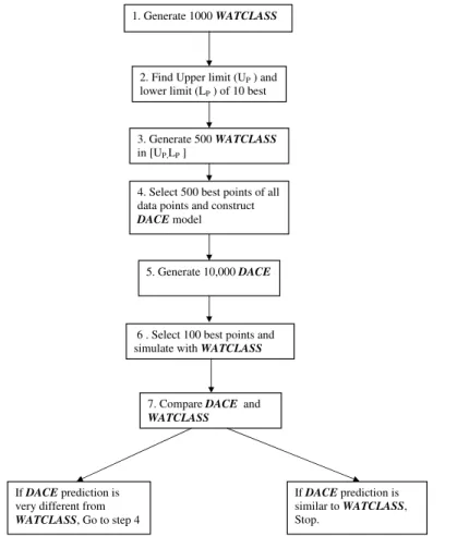
The third set of experiments was focused on approximate model evaluation. This set had two parts. In the first part, 1000 LHS were generated on the input space and

(10)

HESSD

Full Screen / Esc

Printer-friendly Version Interactive Discussion their corresponding NS number was computed.In order to increase the concentration

of points with good prediction (lower error values/higher NS coefficient), 10 best points were selected and in the close vicinity of these points another 500 simulations were performed. This 500 points were located in a hypercube that its edges extend up to the upper bound and lower bound of what that previously 10 selected parameter sets

5

were located. In the second part of the third set of experiment, based on the 500 best results, an approximate model was constructed. This approximate model employed to predict points with NS numbers more than 0.70. So, 10 000 LHS were generated and their corresponding NS coefficients were evaluated by the approximate model. Then, among these 10, 000 points 100 best points were selected. To evaluate the

perfor-10

mance of the approximate model, these best points were simulated with WATCLASS. Then, the estimated results were compared to the simulated results. Deviation of pre-dicted results (from approximate model) from the simulated results (WATCLASS) was the measure for goodness of the approximate model. After 4 iterations (400 points) of approximate model evaluation satisfactory results were achieved. The schematic of

15

the algorithm is shown in Fig. 1. Efficiency of these processes are compared in Ta-ble2. Since the complete process of approximate model construction relies on random sampling of the points, the process replicated 10 times and the mean and standard deviation of approximate model process is reported.

All of the simulations were performed on a “Shared Hierarchal Academic Research

20

Computing Network” Called SHARCNET 2 This service allows the users to conduct hundreds of jobs in parallel.

Comparison of the results shown in Table 2 shows that Latin Hypercube Sampling was slightly more successful in finding points with high NS numbers than random sam-pling (Monte Carlo). Since in LHS all the space has been sampled, the approximate

25

model was constructed based on this sampling method. This way, the entire space of

(11)

HESSD

Full Screen / Esc

EGU

parameters will be explored.

In the first row of Table2, the entire process of DACE approximate model is shown. In the entire process 1900 simulation performed, which only 400 of simulations were based on approximate model prediction. Comparison of LHS and DACE (firts part) shows that on average 24% of points have NS greater than 0.7, whereas in case of

5

LHS method 15% of points have NS number greater than 0.7. In addition to that, standard deviation of the distribution is small.

The results are the same for the rest of NS number intervals, but the standard de-viation is slightly higher correspondingly. However, all of 10 trials in this experiments have better results than LHS and as NS intervals moves to the higher intervals the

10

capability of approximate model to find good points increases. In the second part of DACE, the NS number of 400 points that were simulated based on the approximate model is reported. In this part, 36% of the results are above the first threshold, which is 21% better than LHS. Among all identifying points, 29% were in the next threshold (NS greater than 0.71), but in LHS only 11% of points were in that interval.

15

Overall, DACE method outperformed previous methods in identifying good input sets. DACE model was used to map part of the input space that seemed to contain more acceptable outputs. Model precision increased in each iteration until the error criteria met. This experiment continued for 4 iterations. DACE has the potential of being adapted with any other model, for example neural network or spline can be one of the

20

cases for the approximate model.

The other advantage of DACE is its adaptability with other optimization methods. This technique is not only permits user to employ other types of optimization meth-ods such as GA or SA, but also can be combined with any of these methmeth-ods in an efficient way. For instance, one of the main disadvantages of these population based

25

techniques is being computationally expensive especially when the dimension of the space is high. However, if the input space shrinks by using DACE (smaller parame-ter inparame-tervals, in this case input inparame-terval became 50% of the original input inparame-terval), the computational cost will be definitely less.

(12)

HESSD

Full Screen / Esc

4 Conclusions

he goal of this research was to evaluate the performance of DACE for hydrologic model calibration. Number of acceptable points corresponding to different methods were com-pared and the results are reported in Table2.

This experiment showed promising results for calibration of a small watershed (in

5

North American term). Application of DACE along with LHS reduced the computa-tional cost of calibration process. For example, in this experiment, each WATCLASS simulation took 8 min. Therefore, finding 100 points with NS number greater than 0.7 using LHS method will take 5152 min if the process is completely serial, whereas using DACE for the same case will take only 3360 min. So that, the overall computational

10

cost will be 35% less.

DACE could be combined well with clustering techniques and this way the modeling process will be done on the part of the space that contains acceptable points. This way, the computational expenses will be even less by being more concentrated on the region of interest and getting less sample from other part of the space. It could be also

15

combined with dimensionality reduction techniques and work in a lower dimension. So, the dimension of the modeled space will be smaller (much smaller).

In general, this technique showed the potential of working with any expensive opti-mization problem, such as calibration of the hydrologic models over large watershed.

References

20

Jones, D. R., Schonlau, M., and Welch, W. J.: Efficient Global Optimization of Expensive Black-Box Functions, J. Global Optimization, 13, 455–492, 1998. 2311

Duan, Q., Sorooshian, S., and Gupta, V.: Effective and efficient global optimization for concep-tual rainfall-runoff models, Water Resour., 4, 1015–1031, 1992. 2309

(13)

HESSD

Full Screen / Esc

EGU

Scheme CLASS with the Distributed Hydrological Model WATFLOOD, Atmos.-Ocean, 38, 251–269, 2000. 2310

Fraser, A. and Burnell, D.: Computer Models in Genetics, McGraw-Hill, New York, 1970.2309 Kouwen, N.: WATFLOOD: A micro-computer based flood forecasting system based on

real-time weather radar, Can. Water Resour. J., 13, 62–77, 1988. 2310

5

Krige, D.: A statistical approach to some mine valuations and allied problems at the Witwater-srand, Can. Water Resour. J., 13, 62–77, 1988. 2312

Marsden, A. L., Wang, M., Dennis Jr., J., and Moin, P.: Optimal Aeroacoustic Shape Design Using the Surrogate Management Framework, Optimization and Engineering, 5, 2004.2311 McKay, M., Conover, W., and Beckman, R. J.: A Comparison of Three Methods for Selecting

10

Values of Input Variables in the Analysis of Output from a Computer Code., Technometrics, 21, 239–245, 1979.2314

Metropolis, N., Rosenbluth, A., Rosenbluth, M., Teller, A., and Teller, E.: Equation of State Calculations by Fast Computing Machines., J. Chem. Phys., 21, 1087–1092, 1953. 2309 Mugunthan, P. and Shoemaker, C.: Assessing the impacts of parameter uncertainty for

com-15

putationally expensive groundwater models., Water Resour. Res., 42, 2006. 2311

Mugunthan, Pradeep, S. C. A. R. R. G.: Comparison of function approximation, heuristic, and derivative-based methods for automatic calibration of computationally expensive groundwa-ter bioremediation models, Wagroundwa-ter Resour. Res., 41, 1–7, 2005. 2311

Nash, J. and Sutcliffe, J. V.: River flow forecasting through conceptual models part I A

discus-20

sion of principles, J. Hydrol., 10, 282-290, 1970. 2314

Verseghy, D. L.: CLASS-A Canadian Land Surface Scheme for GCMs, I. Soil Model, Int. J. Climatol., 11, 111–133, 1991. 2310

(14)

HESSD

Full Screen / Esc

Printer-friendly Version Interactive Discussion Table 1. WATCLASS Parameter description.

Parameter Description Lower Bound Upper Bound

drnrow Drainage index for layer 1 0 1

wfcirow An interflow index (mean of KSATa) for layer 1 0 20

sand11 volume of sand in layer1 landclass1 0 100

clay11 volume of clay in layer1 landclass1 0 100

wfcirow interflow index (mean of KSAT)for layer 2 0 20

wfcirow interflow index (mean of KSAT)for layer 3 0 20

a

(15)

HESSD

Full Screen / Esc

EGU

Table 2. Comparison of mean of number of simulations for different methods.

Nash Coefficient Method Number of simu-lations >0.7 >0.71 >0.72 >0.73 Monte Carlo 10000 1300 1011 380 18 LHS 5000 776 561 198 7

DACEa(First Part)mean value 1900 450 360 148 12

DACE(First part)standard deviation 1900 2.5 5 19 6

DACE (Second Part)mean 400 144 118.5 48.8 12.6

DACE(Second part)standard deviation 400 2.6 4.8 10.5 12.9

a

value with polynomial fit function

(16)

HESSD

Full Screen / Esc

1. Generate 1000 WATCLASS

2. Find Upper limit (UP ) and lower limit (LP ) of 10 best

3. Generate 500 WATCLASS in [UP,LP ]

4. Select 500 best points of all data points and construct DACE model

5. Generate 10,000 DACE

6 . Select 100 best points and simulate with WATCLASS

7. Compare DACE and WATCLASS

If DACE prediction is very different from WATCLASS, Go to step 4

If DACE prediction is similar to WATCLASS, Stop.