CONTROL OF AN ARTIFICIAL MOUTH PLAYING A TROMBONE AND ANALYSIS OF SOUND DESCRIPTORS ON EXPERIMENTAL DATA

HAL Id: hal-01245388

https://hal.archives-ouvertes.fr/hal-01245388

Submitted on 17 Dec 2015

HAL is a multi-disciplinary open access

archive for the deposit and dissemination of

sci-entific research documents, whether they are

pub-lished or not. The documents may come from

teaching and research institutions in France or

abroad, or from public or private research centers.

L’archive ouverte pluridisciplinaire HAL, est

destinée au dépôt et à la diffusion de documents

scientifiques de niveau recherche, publiés ou non,

émanant des établissements d’enseignement et de

recherche français ou étrangers, des laboratoires

publics ou privés.

CONTROL OF AN ARTIFICIAL MOUTH PLAYING

A TROMBONE AND ANALYSIS OF SOUND

DESCRIPTORS ON EXPERIMENTAL DATA

Nicolas Lopes, Thomas Hélie, René Caussé

To cite this version:

Nicolas Lopes, Thomas Hélie, René Caussé. CONTROL OF AN ARTIFICIAL MOUTH PLAYING A

TROMBONE AND ANALYSIS OF SOUND DESCRIPTORS ON EXPERIMENTAL DATA.

Stock-holm Music Acoustics Conference 2013, Jul 2013, StockStock-holm, Sweden. �hal-01245388�

CONTROL OF AN ARTIFICIAL MOUTH PLAYING A TROMBONE AND

ANALYSIS OF SOUND DESCRIPTORS ON EXPERIMENTAL DATA

Nicolas Lopes

IRCAM-CNRS-UPMC, UMR 9912, 1 place Igor Stravinsky,

75004 Paris, France nicolas.lopes@ircam.fr

Thomas H´elie

IRCAM-CNRS-UPMC, UMR 9912, 1 place Igor Stravinsky,

75004 Paris, France thomas.helie@ircam.fr

Ren´e Causs´e

IRCAM-CNRS-UPMC, UMR 9912, 1 place Igor Stravinsky,

75004 Paris, France rene.causse@ircam.fr

ABSTRACT

This paper deals with a robotized artificial mouth adapted to brass instruments. A technical description of the robotic platform is drawn, including calibrations, initialization pro-cesses, and modes of control. An experimental protocol is proposed and the repeatability is checked. Then, exper-iments are conducted on a trombone for several types of quasi-static controls. Sound descriptors (fundamental fre-quency, roughness, energy) of measured acoustic signals are estimated and used to build cartographies indexed by the control inputs. An analysis reveals that several stable notes can easily be reached using a basic mapping with respect to these control inputs. However, a histogram of fundamental frequencies shows that some notes in the high range that can be played by musicians are not reached by the artificial mouth. It also reveals that some notes are dif-ficult to play in the middle range. This exploration sug-gests some possible improvements of the machine that are finally discussed.

1. INTRODUCTION

Brass wind instruments are self-sustained musical instru-ments. Their self-oscillations are due to the non-linearity of the aero-elastic valve, namely, the jet coupled to the lips, which is loaded by the acoustic resonator. But, al-though the musician’s control of the valve is crucial, it is very difficult to study this bio-physical system and to make “in vivo” measurements. For this reason, artificial mouths have been developed, see e.g. [1–5].

This paper deals with a robotized version a such systems. This robotization was initiated during the CONSONNES project [6]. It also involved mechatronic projects in an en-gineering school [7] and several internships [8–11]. Some first results and evolutions of the machine functionalities have been presented in [12–14]. In the last one, it has been showed that sequences of a few trumpet notes could be played with a simple open loop control, using a “hand-tuned” mapping based on a sound descriptor analysis1_.

1_{A movie can been downloaded on the following website:}

http://recherche.ircam.fr/anasyn/helie/Brasstronics/FilmBrasstronics2011.avi

Copyright: c 2013 Nicolas Lopes et al. This is an open-access article distributed under the terms of theCreative Commons Attribution 3.0 Unported License, which permits unrestricted use, distribution, and reproduction in any medium, provided the original author and source are credited.

In this paper, a systematic approach is proposed and based on (1) calibrations and initialization processes, (2) an ex-perimental protocol and repeatability tests, and (3) sets of cartographies of sound descriptors (with respect to quasi-static inputs) for several modes of control. It allows char-acterizing notes that can be easily played, and to exhibit some limitations of the machine as well as some dyssym-metry between the lips.

This paper is organized as follows. Section 2 gives an overview of the robotic platform, its sensors and actuators. Section 3 is devoted to the calibration of some sensors and to the configuration of the machine. This includes initial-ization processes and feedback-loop controller settings. In section 4, an experimental protocol is proposed and the re-peatability is checked. Then, the first experimental results obtained for a single control variable are presented in sec-tion 5. They allow the establishment of a partial but robust mapping based on a sound descriptor analysis. Section 6 extends these results to 2D cartographies for various con-trol modes with multiple inputs. In particular, the playing frequencies of the set of all cartographies are examined and compared to the impedance peaks of the trombone. This analysis suggests some possible improvements of the ma-chine that are discussed in section 7 with conclusions and perspectives.

2. TECHNICAL DESCRIPTION

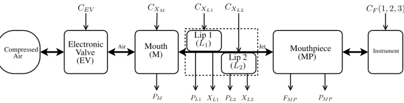
The robotic platform is composed of three principal parts : (1) the air supply, (2) the artificial mouth with two lips and (3) the brass instrument with artificial fingers. It includes a set of height actuators, fourteen sensors, interfaced with a DSP setup and a computer to control the machine. 2.1 Mechanical parts

The mouth (M) is a ≃80cm3

chamber, which is fed by a controlled air supply. It is ended by two vertical artificial lips (L1, L2). Each lip is a cylindrical latex chamber filled

of water. The brass instrument (in this work, a valve trom-bone) with its mouthpiece (MP) is fixed close to the mouth. The contact of the lips with the mouthpiece is ensured by controlling the position of the (mobile) mouth. Three arti-ficial fingers can be used to push on the trombone valves. These components and their coupling are represented in figure 1.

Lip 1 (L1) Lip 2 (L2) Mouth (M) Mouthpiece_(MP) Compressed Air Electronic Valve (EV) CEV XL1 XL2 FM P PM P PM PL1 PL2 CXM CXL1 CXL2 CF(1, 2, 3) Instrument Jet Air

Figure 1. Block diagram of the robotized platform.

2.2 Actuators

The input airflow is controlled by an electronic valve (EV), here, a B¨ı¿12rkertproduct (Type 6022). The mouth

dis-placement is driven by a SMAC linear actuator (LAL95-050-75F/LAA-5). The water volume inside each lip is provided by a hydraulic cylinder, also driven by a SMAC linear actuator (LAL35-015-75/LAA-5). These linear ac-tuators are all moving coils that deliver a (Laplace) force which is proportional to the input voltage. Artificial fingers are built with simple (On/Off) electromagnets. Addition-ally, a horn loudspeaker can be plugged at the top of the mouth, for active acoustic control issues (see [15]). The results presented below do not involve this device but its use is considered in perspectives.

Note that the inputs of these actuators are all represented and labeled at the top of figure 1.

2.3 Sensors

The position of each linear actuator (XM for the mouth,

XL1 and XL2 for the lips, see figure 2) is measured by

a built-in incremental encoder with a step of5 × 10−6_m.

The (static and acoustic) air pressure in the mouth (PM) is

measured by an Endevco sensor (8507-5). A second simi-lar sensor (8507-2) is used for the mouthpiece (PM P). The

(static) water pressure (PL1, PL2) is measured at the top

of each lip (same altitude) by two Kistler sensors (RAG-25R0.5BV1H). A SMD force sensor (S215) is localized between the mouthpiece and the instrument to measure the force (FM P) applied by the lips to the mouthpiece.

XM XL1 XL2 PL1 PL2 PM PM P FM P CEV Actuator hydraulic cylinder

Figure 2. Sketch of the artificial mouth with its main actu-ators and sensors.

These sensors include built-in electronic signal condition-ers except for PM, PMP and FMP, which are conditioned

with a low power instrumentation amplifier (INA 118). Moreover, we performed home-made calibrations of these sensors, except for the Endevco devices (PM, PM P) which

received a factory calibration certificate. These calibra-tions are described in § 3.1.

Note that the outputs of the height sensors described above are all represented and labeled at the bottom of figure 1. The additional six sensors mentioned at the beginning of section 2 are: one high pressure sensor localized upstream of the electro-valve, three temperature sensors, one optical intensity sensor for estimating the opening area between the lips, and one microphone localized at the bell of the instrument. These additional sensors are not directly ex-ploited in this paper.

2.4 Interface

The transducers associated with audio frequency ranges are connected to a sound card (see figure 3). Other trans-ducers (with a lower frequency range) are connected to a dSpace c system, composed of an input/output inter-face and a Digital Signal Processor (DSP). The DSP is programmed using a dSpace software associated with a Matlab-Simulink-RTW c environment. It is used to de-sign some (low-level) feedback loop controllers applied to the actuators. Real-time analysis of audio signals (fun-damental frequencies, energy, etc) are performed by the MAX/MSP software. High-level controls of the robot (ini-tializations, automated experiments, etc) are performed by Python scripts under the dSpace ControlDesk environment which communicates with MAX/MSP c .

Robot T ra n sd u ce rs Sound card dSpace interface DSP MAX / MSP ControlDesk / Python: * Graphic interface * Communication * Scripts and processes

Matlab / Simulink / RTW

Computer

synchro. signal

3. CALIBRATION AND CONFIGURATION The section deals with: (1) the calibration of the force sensor (FM P) and the water pressure sensors (PL1, PL2),

(2) the initialization of the zero positions of the linear ac-tuators (XL1, XL2and XM) so that this reference

corre-sponds to a robust reference state of the lips, (3) the de-velopment and the adjustment of feedback loops to control linear actuators with respect to chosen command variables (possibly different from the natural one, the Laplace force). 3.1 Calibrations

The force and the water pressure sensors are low-frequency range sensors. We perform their calibration for quasi-static configurations. The force sensor is calibrated using gravity and reference masses (precision: ±0.1g) based on an in-cremental mass step of50g. For the water pressure sensors, a one-meter vertical water column is used, at the bottom of which the two sensors are simultaneously connected (same altitude, see figure 4). An incremental height step of five centimeters is used, corresponding to a 5 × 102

P a sam-pling precision for the pressure.

Water pressure sensor PL1 Water pressure sensor PL2

Water column

Figure 4. Schema of the water pressure sensors calibra-tion. Static calibration based on a variable water column

The linearity of the three sensors was confirmed and the sensitivities measured.

3.2 Initialization processes

3.2.1 Zero positions for XL1and XL2

A lip (L) is a cylindrical latex chamber with natural volume Vref_{. When the water volume V}

L is smaller than V_Lref,

the latex is not stressed. In the opposite situation (VL >

VLref), the latex stress makes the water pressure increase.

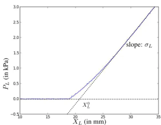
This effect is measured by making the position XLslowly

increase from the forward to the backward trip points of the actuator2_{. We observe on the measure (see figure 5)}

that, except in the vicinity of VLref, these two behaviors can

be approximated by one constant pressure for VL< V_Lref

and an affine function with slope σ (Pa/m) for VL> V ref

L .

The zero position of XL= X 0

L= 0 is chosen and adjusted

to correspond to the intersection point of the two straight lines.

Note that XL = 0 does not match with V ref

L . But, it

splits the curve into two affine asymptotic behaviors and defines a more robust initialization (see table 1 in § 4.2 for

2_{The volume variation equals the position variation multiplied by the}

section of the hydraulic cylinder.

XL(in mm) PL (i n k P a) slope: σL X0 L

Figure 5. Measured water pressure PL1with respect to the

position XL1 when the second lip L2 is deflated and the

mouthpiece is out of contact (Mouth in retracted position) and estimation of its piecewise linear approximation.

ten repetition tests). This initialization is performed for each lip, independently, and with no airflow.

3.2.2 Zero position for XM

Once the zero positions of the lips are estimated, that of the mouth is adjusted using a similar principle. In this case, the measured quantity is the force (FM P) (rather than the

wa-ter pressure) while the lips are filled with their reference volume (XL1 = XL2 = 0). The measurements are

dis-played in figure 6. XM(in mm) FM P (i n ≡ g ) slope: σM X0 M

Figure 6. Measured force FP M with respect to the

posi-tion XM when the lips are filled with their reference

vol-ume and estimation of its piecewise linear approximation.

Note that XM= 0 does not match with the contact point

between the lips and the mouthpiece, but this initialization is chosen for its robustness properties, as for XL= 0.

For experiments, typical positions correspond to slightly crushed (XM >0) non over-inflated (XL<0) lips, such

that the contact is established (FM P>0). In practice, this

facilitates the formation of a buzz, or at least, that of an airflow path between the lips even for low static pressure in the mouth.

3.3 Feedback loop controllers and modes of control The linear actuators are not naturally controlled with re-spect to the position but (proportionally to) the Laplace force. To achieve a control in position, we use standard tools of automatic control, here, some Proportional-Integral-Derivative (PID) controllers. Digital versions of these con-trollers are designed under the Matlab/Simulink/RTW en-vironment and tuned following classical methods (see e.g. [16]). They are implemented in the DSP card of the dSpace system. For the control in position, typical performances are about 50ms. Other control types (in FM P, PL1or PL2)

are available and also based on PID controllers.

In this paper, several modes of control of the lips are con-sidered. They consists of choosing, for each linear actu-ator, a control of position type or of force/pressure type. But, not all the combinations are compatible: positions are independent variables but, because of the contact between the lips and the mouthpiece, the force and the water pres-sures are linked. Here, we consider modes of control which include no more than one input of force/pressure type: (XM, XL1, XL2) this mode controls variables which do

not depend of the system state;

(FM P, XL1, XL2) this mode is well-adapted to control the

contact quality between the lips and the mouthpiece; (XM, PL1, XL2) this mode (or its symmetrical version)

allows the study of the effect due to the stress of one particular lip.

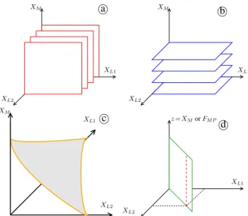
The feasibility of these three modes is confirmed and the repeatability is tested in section 4. Moreover, in sections 5 and 6, the two first modes are used, combined with the air-flow supply, to explore self-oscillations. They allow the au-tomatic generation of cartographies of sound descriptors, following the curves or the surfaces detailed in figure 7.

4. EXPERIMENTAL PROTOCOL AND REPEATABILITY

In this section, we propose: (1) a protocol adapted to the quasi-static experiments presented in section 5 and sec-tion 6, (2) a repeatability test.

4.1 Protocol

An experiment is processed choosing a mode of control, an exploratory subspace, and following a precise proto-col. The subspace is explored with quasi-static commands. To ensure quasi-static states, waiting times are added be-tween measurements. For each measured point, every data from all sensors (Temperatures, Pressures, Positions, etc) are recorded and saved. Moreover, acoustic signals are au-tomatically analyzed using tools provided by the MIR tool-box [17, 18]. For all measured points, sound descriptors such as fundamental frequency (if any), sound energy and roughness are estimated and saved. The protocol consists of the following steps:

1. Measurement of the idle-state of the machine

a XM XL1 XL2 b XM XL1 XL2 c XM XL1 XL2 d z= XMor FM P XL1 XL2

Figure 7. Modes of control of the three linear actuators combined with partitions of 3D spaces Subfigures a - b illustrate two types of partition of the 3D space into 2D pla-nar subspaces, for the mode of control(XM, XL1, XL2).

Subfigure c illustrates a FM P-constant surface. It is

ob-tained with the mode of control(FM P, XL1, XL2) where

the first input is a fixed value. Subfigure d describes a symmetrical control of the lips (XL1= XL2) for a fixed

value XL1 (1D-space: red dashed straight line) or on a

range (2D-space: green plane). The very first exploration in § 5 is obtained by using the 1D control subspace in d with z= FM P, and the 2D cartographies in § 6 by using

the 2D spaces described in a - c and d with z= XM.

2. First initialization process: measurement of X0 M, X

0 L1,

X0

L2, σM, σL1and σL2.

3. For each desired point of measurement in the sub-space:

(a) The chosen position (or force/pressure) com-mand are set up;

(b) First waiting: a0.5s waiting is imposed to en-sure actuators positions;

(c) Breath activation: CEV goes from0 (close

po-sition) to a reference (here,35% of the maxi-mal aperture);

(d) Second waiting: a1s waiting is imposed to en-sure a quasi- stationary regime;

(e) Measurements are recorded and saved. 4. Second initialization process.

5. Measurement of the static pressures and the temper-atures of the machine.

Parameters that are estimated during steps 2 and 4 are saved. They are compared to validate the constancy of the lips behavior. More precisely, the deviations of σM, σL1 and

σL2 characterize the latex fatigue due to an experiment.

The deviations of X0 M,X

0

L1 and X 0

L2 allow the detection

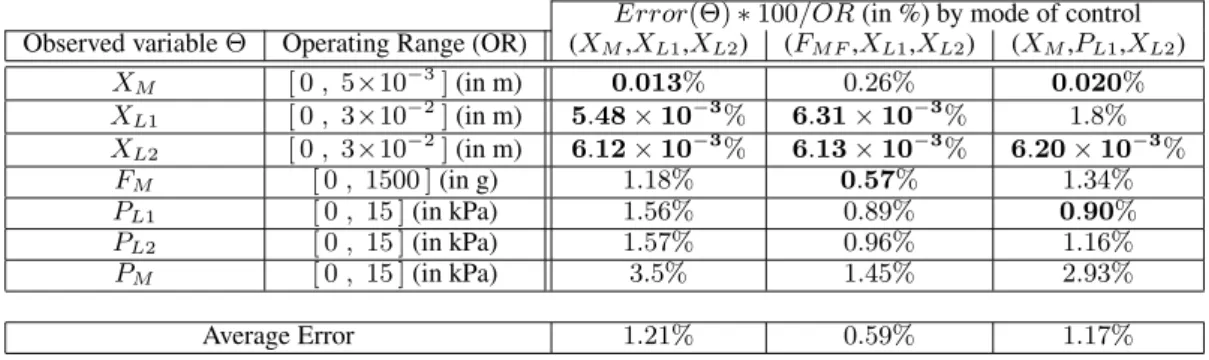
Error(Θ) ∗ 100/OR (in %) by mode of control Observed variableΘ Operating Range (OR) (XM,XL1,XL2) (FM F,XL1,XL2) (XM,PL1,XL2)

XM [ 0 , 5×10− 3 ] (in m) 0_{.013% 0.26%} 0_.020% XL1 [ 0 , 3×10− 2 ] (in m) 5_{.48 × 10}−3_% 6_{.31 × 10}−3_{% 1.8%} XL2 [ 0 , 3×10− 2 ] (in m) 6_{.12 × 10}−3_% 6_{.13 × 10}−3_% 6_{.20 × 10}−3_% FM [ 0 , 1500 ] (in g) 1.18% 0.57% 1.34% PL1 [ 0 , 15 ] (in kPa) 1.56% 0.89% 0.90% PL2 [ 0 , 15 ] (in kPa) 1.57% 0.96% 1.16% PM [ 0 , 15 ] (in kPa) 3.5% 1.45% 2.93% Average Error 1.21% 0.59% 1.17%

Table 1. Errors relative to the operating range (OR), measured with the repeatability tests (Ni= 10, Nk= 4 × 4 × 4 = 64)

for three modes of control. Values in bold correspond to the controlled variables.

4.2 Repeatability tests

To evaluate the repeatability of an experiment based on the protocol seen above, we perform a test for each mode of control presented in section 3. Ni identical experiments

are processed. Experiments explore a set of Nkpoints that

are fixed and distributed in the 3D-space. Between each experiment, the initialization parameters are manually dis-turbed: some water is added or removed in the “water cir-cuit” and the instrument is slightly displaced (by hand).

Measurements are compared and analyzed, based on the following definitions:

1. A variableΘ measured at point k during experiment i is denotedΘi

k whereΘ can be a measurement on a

sensor with a low frequency range (FM P, XM, etc),

or a parameter estimated on a stationary signal (typ-ically, a sound descriptor, see below).

2. For a given point k, the expected value E(Θk) is

es-timated by its average on the Niexperiments, namely,

E(Θk) ≈ 1 Ni Ni X i=1 Θi k.

3. The standard deviation is correspondingly estimated by

s(Θk) =

q E(Θ2

k) − E(Θk)2.

4. The standard deviation of a variableΘ, averaged on the Nkexperimental points, is denoted

Error(Θ) = 1 Nk Nk X k=1 s(Θk).

Results are presented in table 1 for the measurements of positions, water pressures and the force FM P. In this

ta-ble, to make the comparison between variables easier, the error is normalized with the (amplitude of the) operating range. The results show that the protocol and the initializa-tion process are accurate enough to guarantee and quantify the repeatability for quasi-static experiments. Note that the mode of control based on the force (FM F,XL1,XL2)

appears to be, globally, the most efficient: it reduces the average error. Moreover, for this mode of control, the last step of the initialization process is not required.

5. FIRST EXPERIMENT WITH A SINGLE CONTROL VARIABLE

5.1 Global considerations

At low order, the musician’s lips can be approximated by mass-damper-spring mechanical systems [4]. Here, these 3 × 2 macro-parameters are related to the 3 control inputs (see figure 7), making them linked together. For instance, for a fixed position XM (figure 7, mode b ), the

varia-tion of the (oscillating part of the) mass Mk of the lip Lk

nearly equals that of the water displaced by XLk. The

vari-ations of stiffness Kkand damping Dkare more complex

to model. Their measurement is not straightforward, even at a static equilibrium. This is why in e.g. [3, 4], these parameters are (at least partially) estimated, by analyzing the natural frequency of buzzes. In this paper, we simply explore the variability of regimes by modifying the control inputs: several frequencies can actually be reached because the sensitivities of parameters(Mk, Dk, Kk) w.r.t the

con-trol inputs are not proportional. The experiment described below makes a first exploration of regimes for a simple 1D control.

5.2 Description of the experiment

The 1D control is chosen so that the lips are in a symmet-rical configuration. In order to makes this configuration as robust as possible, the independent variables XL1 = XL2

are kept constant and fixed to −15mm, and the mouth con-trol is chosen to be FM P which increases from100g to

1000g, following the protocol described in § 4.1. 5.3 Measurements and observations

Figure 8 shows the measured force FM P and signal

de-scriptors [17, 18] of the acoustic pressure measured in the mouthpiece PM P. The three sub-figures respectively

dis-play: (1) the force, (2) the fundamental frequency f0 of

PM P, estimated by the YIN algorithm [18], and (3) the energyof the signal. An additional curve representing the

roughnessis superposed to the estimated fundamental fre-quency. The roughness is defined without unit: a high value means that the signal is not harmonic.

This figure validates that several fundamental frequencies are reachable. The analysis of sound descriptors clearly al-lows the extraction of connected areas of self-oscillating

regimes for which the roughness is low and the energy is high. These areas correspond to some “stable notes”. The complementary areas basically correspond to non-oscillating or complex signals (multiphonics, chaos, etc). Complex signals are mainly located in thin transition areas between stable notes.

5.4 First conclusion

This experiment shows that the robotic platform is able to produce various self-oscillating regimes including stable

notes. For stable notes, it appears that, to a large extent, the higher the force FM P, the higher the fundamental

fre-quency. Moreover, stables notes and their areas are suffi-ciently reproducible to map some control input values to fundamental frequencies. Next section extends this explo-ration to the case of two control inputs.

6. TWO-DIMENSIONAL CARTOGRAPHIES In this section, four experiments are set up, based on the modes of control a to d in figure 7.

6.1 Description of the experiments

Experiments are conducted following the protocol in § 4.1. For each experiment, the control inputs are specified below with their exploration range and the incremental step. Vari-ables are sorted as follows: the first, second and third ones respectively correspond to (1) a constant value (except in case d ), (2) a slow increasing sweep, and (3) a faster (but still quasi-static) increasing sweep. Parameters are: Mode a : XL2= −15mm; 1mm ≤ XM ≤4mm (step: 0.1mm); −30mm ≤ XL1≤0mm (step: 0.5mm); Mode b : XM = 3.5mm; −30mm ≤ XL2 ≤ 0mm (step: 0.5mm); −30mm ≤ XL1 ≤ 0mm (step: 0.5mm); Mode c : FM P≡500g; −30mm ≤ XL2 ≤0mm (step: 0.5mm); −30mm ≤ XL1≤0mm (step: 0.5mm); Mode d : 1mm ≤ XM ≤4mm (step: 0.1mm); XL1= XL2with −30mm ≤ XL1≤0mm (step: 0.5mm).

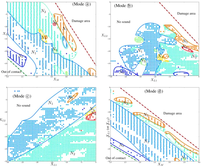
6.2 Measurements: comments and observations The results of these four experiments are given in figure 10. For each mode of control, a - d , connected areas associ-ated with “stable notes” can still easily be extracted. How-ever, these 2D cartographies makes some complexity ap-pear: they include non convex areas and a large variety of sizes, specially for modes a and b . The experiment for mode d ) is an extension of that shown in section 5. We can observe wide diagonal bands of stable note areas so that mode d makes the note selection simpler than other modes. Indeed, a preferred axis can be selected (such as XLproportional to XM) in order to explore areas of stable

notes with increasing frequencies.

Sub-figure c displays a few number of huge or confined areas, meaning that the force is well adapted to stabilize some specific notes (here, denoted N1 and N2).

Y Frequencies (in Hz) N0 N1 N2 N3 N 4 N5 N6

Figure 9. Normalized histogram of fundamental frequen-cies superposed to the modulus of the input impedance measured with the BIAS system [20].

However, note that, the symmetry with respect to lips 1 and 2 is not satisfied, although initializations are correct (and their reproducibility is checked). This can also be observed in sub-figure b . This issue will require a special attention in a future work.

Moreover, the histogram in figure 9 shows that the seven first notes of the instrument (N0to N6) can be played. We

can notice that playable frequencies perfectly fit with the trombone impedance (green solid line curve) but are lo-cated at the right of each peak (as expected [19]).

7. CONCLUSIONS AND PERSPECTIVES In this paper, a robotized artificial mouth dedicated to play-ing the brass instruments is described with its mechatronic parts, its calibration, some robust initialization processes and several modes of control. Repeatability tests (ten ac-quisitions for each mode of control) is performed to es-timate the standard deviation on the measured variables which characterize the lips in quasi-static configurations. Globally, the relative deviation proves to be less than 0.9% for the controlled variables and less than 3.5% for the un-controlled ones. A protocol for experiments is proposed. In particular, it records the temperature during a (possibly long) experiment and characterizes the latex fatigue. Ex-periments on a trombone are designed to build cartogra-phies for several modes of (quasi-static) control. These cartographies display sound descriptors (fundamental fre-quency, roughness, energy) as a function of the control input values. This exploration reveals that several stable notes can easily be reached using a basic mapping but that notes in the high range of the instrument cannot be played by the artificial mouth.

To cope with this limitation, a perspective is to modify the machine in order to make it able to play notes in the high register. A solution could consist of controlling the acoustic impedance of the mouth. A partial but encour-aging result based on an acoustic active control can be found in [15]. In this work, the RMS pressure amplitude is analyzed with respect to the (controlled) phase differ-ence between the pressure in the mouth and in the

mouth-Time(s) Time(s) Time(s) FM f0 E n e r g y (d B ) N1 N1 N1 N2 N2 N5

Figure 8. (First experiment: XL1 = XL2 = −15mm and FP M increasing from100g to 1000g) Top: FM w.r.t. time.

Middle: fundamental frequency estimated on the acoustic signal PM P (·) and roughness (-). Bottom: signal energy. In this

figure, the color map corresponds to the frequencies and areas with stable notes are emphasized with boxes.

XL1 XM N0 N1 N2 N3 N4 N5 N6 (Mode a ) Damage area Out of contact XL1 XL2 N0 N1 N2 N3 N4 N5 N6 Damage area No sound (Mode b ) XL1 XL2 N1 N2 N4 N5 N6 No sound (Mode c ) XL 1 (o r XL 2 ) XM N0 N1 N2 N3 N5 Out of contact Damage area (Mode d )

Figure 10. 2D-cartographies for various control modes. Top left: mode (XM,XL1,XL2) with constant XL2. Top right:

mode (XM,XL1,XL2) with constant XM. Bottom left: mode (FM P,XL1,XL2) with constant FM P. Bottom right: mode

(XM,XL1= XL2). The color map corresponds to the frequencies (see figure 9) and stable note areas are surrounded. The

red dotted line represents the security limit (PL1 > 15kP a or PL2 > 15kP a) and the green dotted line represents the

piece. A second perspective concerns the study of some macro-mechanical parameters of the lips (effective mass M , damping D and stiffness K) with respect to the con-trol inputs. However, note that the (3D) concon-trol inputs do not allow the setting of the (3 × 2) macro-parameters. A first approach is to hold up one lip (its 1D control is then used to ensure the air-tightness). The 2D remaining con-trol inputs can then be used to tune two of the three macro-parameters of the other (vibrating) lip, typically, M and K. A third perspective is to implement some high-level feed-back loop controllers driven by the fundamental frequency and acoustic the energy.

More generally, a complete dynamical system modeling of the machine is under study. The long-term goals of this research are to: (1) derive state observers, (2) design ef-ficient high-level controllers, and (3) build inversion pro-cesses to make the machine play target sound waves.

Acknowledgments

Authors wish to thank the French National Research Agency and the project CAGIMA for supporting this work and Alain Terrier and G¨ı¿12rard Bertrand for their technical

as-sistance.

8. REFERENCES

[1] C. Vergez and X. Rodet, “Comparison of real trum-pet playing, latex model of lips and computer model,” in ICMC: International Computer Music Conference, Thessanoliki Hellas, Greece, Septembre 1997, pp. 180–187.

[2] ——, “Experiments with an artificial mouth for trum-pet,” in ISMA: International Symposium of Music

Acoustics, Leavenworth, Washington state USA, Juin 1998, pp. 153–158.

[3] J. Gilbert, S. Ponthus, and J.-F. Petiot, “Artificial buzzing lips and brass instruments: experimental re-sults,” J. Acoust. Soc. Am., vol. 104, no. 3, pp. 1627– 1632, 1998.

[4] J. Cullen, J. Gilbert, and D. M. Campbell, “Brass in-struments : linear stability analysis and experiments with an artificial mouth,” Acta Acustica united with

Acustica, vol. 86, no. 3, pp. 704–724, 2000.

[5] J.-F. Petiot, F. Teissier, J. Gilbert, and M. Campbell, “Comparative analysis of brass wind instruments with an artificial mouth: First results,” Acta Acustica united

with Acustica, vol. 89, no. 6, pp. 974–979, 2003. [6] J. Kergomard, “Projet consonnes: Contrˆole des

sons naturels et synth´etiques,” Agence Nationale de la Recherche (ANR-05-BLAN-0097-01), 2005-2009, http://www.consonnes.cnrs-mrs.fr/.

[7] “Mechatronics projects of the engineering school of mines paristech,” http://www.mecatro.fr/.

[8] B. V´ericel, “Commande et interfac¸age d’un robot mu-sicien,” 2009.

[9] ——, “Confrontation th´eorique/exp´erimentale de caract´eristiques d’excitation dans le jeu des cuivres,” 2010. [Online]. Available: http://articles.ircam.fr/textes/Vericel10a/

[10] N. Lopes, “Cartographie de param`etres de jeu de trompettiste: mise en correspondance automatique du son produit avec les param`etres de contrˆole d’une bouche artificielle asservie,” 2011. [Online]. Available: http://articles.ircam.fr/textes/Lopes11a/

[11] ——, “Mod´elisation, asservissement et com-mande d’une bouche artificielle robotis´ee pour le jeu des cuivres,” 2012. [Online]. Available: http://articles.ircam.fr/textes/Lopes12a/

[12] D. Ferrand, T. H´elie, C. Vergez, B. V´ericel, and R. Causs´e, “Bouches artificielles asservies: ´etude de nouveaux outils pour l’analyse du fonctionnement des instruments `a vent,” in Congr`es Franc¸ais d’Acoustique, vol. 10, Lyon, France, Avril 2010. [Online]. Available: http://articles.ircam.fr/textes/Ferrand10a/

[13] T. H´elie, N. Lopes, and R. Causs´e, “Robotized arti-ficial mouth for brass instruments: automated experi-ments and cartography of playing parameters,” in

PE-VOC - Pan European Voice Conference, vol. 9, Mar-seille, France, 2011, pp. 77–78.

[14] ——, “Open-loop control of a robotized artificial mouth for brass instruments,” in Acoutics 2012 (ASA), Hong Kong, China, 2012, pp. 1–1.

[15] V. Fr´eour, N. Lopes, T. H´elie, R. Causs´e, and G. Scav-one, “Simulating different upstream coupling condi-tions on an artificial trombone player system using an active sound control approach,” in International

Con-ference on Acoustics, vol. 21, 2013, p. 5p.

[16] K. Astr¨om and T. H¨agglund, PID Controllers: Theory,

Design, and Tuning, 2nd ed. International Society for Measurement and Control, 1995.

[17] O. Lartillot and P. Toiviainen, “A Matlab Toolbox for Musical Feature Extraction from Audio,” in the

10th International Conference on Digital Audio Effects (DAFx07), 2007, pp. 237–244.

[18] A. de Cheveign´e and H. Kawahara, “Yin, a funda-mental frequency estimator for speech and music,” J.

Acoust. Soc. Amer., vol. 111, pp. 1917–1930, 2002. [19] M. Campbell, “Brass instruments as we know them

to-day,” Acta Acustica united with Acustica, vol. 90, pp. 600–610, 2004.

[20] G. Widholm, H. Pichler, and T. Ossmann, “Bias: A computer-aided test system for brass wind instru-ments,” in Audio Engineering Society Convention, vol. 87, 1989, paper 2834.