HAL Id: hal-00392136
https://hal.archives-ouvertes.fr/hal-00392136
Submitted on 5 Jun 2009
HAL is a multi-disciplinary open access
archive for the deposit and dissemination of
sci-entific research documents, whether they are
pub-lished or not. The documents may come from
teaching and research institutions in France or
abroad, or from public or private research centers.
L’archive ouverte pluridisciplinaire HAL, est
destinée au dépôt et à la diffusion de documents
scientifiques de niveau recherche, publiés ou non,
émanant des établissements d’enseignement et de
recherche français ou étrangers, des laboratoires
publics ou privés.
Setting and analysis of the multi-configuration
time-dependent Hartree-Fock equations
Claude Bardos, Isabelle Catto, Norbert j. Mauser, Saber Trabelsi
To cite this version:
Claude Bardos, Isabelle Catto, Norbert j. Mauser, Saber Trabelsi. Setting and analysis of the
multi-configuration time-dependent Hartree-Fock equations. Archive for Rational Mechanics and Analysis,
Springer Verlag, 2010, 198 (1), pp.273-330. �10.1007/s00205-010-0308-8�. �hal-00392136�
TIME-DEPENDENT HARTREE-FOCK EQUATIONS
CLAUDE BARDOS, ISABELLE CATTO, NORBERT J. MAUSER, AND SABER TRABELSI
Abstract. In this paper we formulate and analyze the Multi-Configuration Time-Dependent Hartree-Fock (MCTDHF) equations for molecular systems with pairwise interaction. This is an approximation of the N-particle time-dependent Schr¨odinger equation which involves (time-dependent) linear com-bination of (time-dependent) Slater determinants. The mono-electronic wave-functions satisfy nonlinear Schr¨odinger-type equations coupled to a linear sys-tem of ordinary differential equations equations for the expansion coefficients. The invertibility of the one-body density matrix (full-rank hypothesis) plays a crucial rˆole in the analysis. Under the full-rank assumption a fiber bundle structure shows up and produces unitary equivalence between different useful representations of the approximation. We establish existence and uniqueness of maximal solutions to the Cauchy problem in the energy space as long as the density matrix is not singular for a large class of interactions (including Coulomb potential). A sufficient condition in terms of the energy of the ini-tial data ensuring the global-in-time invertibility is provided (first result in this direction). Regularizing the density matrix breaks down energy conserva-tion. However a global well-posedness for this system in L2 is obtained with
Strichartz estimates. Eventually solutions to this regularized system are shown to converge to the original one on the time interval when the density matrix is invertible.
Multiconfiguration methods, Hartree–Fock equations, Dirac–Frenkel variational principle, Strichartz estimates
1. Introduction
The purpose of the present paper is to lay out the mathematical analysis of the multiconfiguration time–dependent Hartree–Fock (MCTDHF) approximation which is used in quantum chemistry for the dynamics of few electron problems, or the interaction of an atom with a strong short laser-pulse [7, 37, 38] and [21]. The MCTDHF models are natural generalizations of the time-dependent Hartree-Fock (TDHF) approximation, yielding a hierarchy of models that, in principle, should converge to the exact model.
The physical motivation is a molecular quantum system composed of a finite number M of fixed nuclei of masses m1, . . . , mM > 0 with charge z1, . . . , zM > 0
and a finite number N of electrons. Using atomic units, the N -body Hamiltonian of the electronic system submitted to the external potential due to the nuclei is then the self-adjoint operator
(1.1) HN = ! 1≤i≤N " −12∆xi+ U (xi) # + V (x1,· · · , xN)
acting on the Hilbert space L2(ΩN; C) with pairwise interaction between the
elec-trons of the form
V (x1,· · · , xN) =
!
1≤i<j≤N
v(|xi− xj|), 1
with v real-valued. Here and below Ω is either the whole space R3 or a bounded
domain in R3 with boundary conditions. The N electrons state is defined by a
wavefunction Ψ = Ψ(x1, . . . , xN) in L2(ΩN) that is normalized by"Ψ"L2(ΩN)= 1.
To account for the Pauli exclusion principle which features the fermionic nature of the electrons, the antisymmetry condition
Ψ(x1, . . . , xN) = !(σ)Ψ(xσ(1), . . . , xσ(N )),
for every permutation σ of {1, . . . , N} is imposed to the wave-function Ψ. The space of antisymmetric wave-functions will be denoted by$N
i=1L2(Ω). In (1.1) and
throughout the paper, the subscript xi of −∆xi means derivation with respect to
the ith variable of the function Ψ. Next,
U (x) :=− M ! m=1 zm |x − Rm|
is the Coulomb potential created by M nuclei of respective charge z1,· · · , zM >
0 located at points R1,· · · , RM ∈ R3 and v(x) = |x|1 is the Coulomb repulsive
potential between the electrons. Actually our whole analysis carries through to more general hamiltonians (possibly time-dependent) as explained in Section 7 below.
For nearly all applications, even with two interacting electrons the numerical treatment of the time-dependent Schr¨odinger equation (TDSE)
(1.2) i∂Ψ
∂t =HNΨ , Ψ(0) = Ψ
0,
is out of the reach of even the most powerful computers, and approximations are needed.
Simplest elements of$N
i=1L2(Ω) are the so-called Slater determinants
(1.3) Ψ(x1, . . . , xN) = 1 √ N !det%φi(xj) & 1≤i,j≤N
constructed with any orthonormal family φi in L2(Ω) . The factor √1
N ! ensures the
normalization condition on the wave-function. Such a Slater determinant will be denoted by φ1∧. . .∧φN. The family of all Slater determinants built from a complete
orthonormal set of L2(Ω) is a complete orthonormal set of$N
i=1L2(Ω). Algorithms
based on the restriction to a single Slater determinant are called Hartree-Fock approximation (HF). On the other hand the basic idea of the multi-configuration methods is to use a finite linear combinations of such determinants constructed from a family of K(≥ N) orthonormal mono-electronic wavefunctions.
One observes (this computation is done in Subsection 3.5) that in the absence of pairwise interacting potentials any Slater determinant constructed with orthonor-mal solutions φi(x, t) to the single-particle time–dependent Schr¨odinger equation
gives an exact solution of the N -particle non interacting time–dependent Schr¨odinger equation. Such φi(x, t) are called orbitals in the Chemistry literature. The same is
true for any linear combination of Slater determinants with constant coefficients. Of course, the situation turns out to be completely different when pairwise inter-actions are added : a solution to TDSE starting with an initial data composed of one or a finit number of Slater determinants will not remain so for any time t '= 0. Such behaviour (called “explosion of rank”) is part of the common belief, but is not shown rigorously as a property of the equations, to the best of our knowl-edge. In the MCTDHF approach one introduces time–dependent coefficients and time-dependent orbitals to take into account pairwise interactions and to preserve
the finite linear combination structure of Slater determinants in time. Using time-independent orbitals as it corresponds to a Galerkin-type approximation would save the effort for the nonlinear equations, but requires a much larger number of relevant orbitals and hence the numerical cost is much higher. The motion of the electrons in the MCTDHF framework is then governed by a coupled system of K nonlinear partial differential equations for the orbitals and%K
N& ordinary differential equations
for the expansion coefficients (see for instance System (3.27)).
Although MCTDHF is known for decades, the mathematical analysis has been tackled only recently. For a mathematical theory of the use of the time-independent multiconfiguration Hartree–Fock (MCHF) ansatz in the computation of so-called ground– and bound states we refer to [25, 17, 26]. A preliminary contribution was given by Lubich [28] and Koch and Lubich [24] for the time-dependent multi-configuration Hartree (MCTDH) equations for bosons, for the simplified case of a regular and bounded interaction potential v between the electrons and a Hamilton-ian without exterior potential U . The MCTDH equations are similar to MCTDHF from the functional analysis point of view, although more complicated from the algebraic point of view, since more density-matrices have to be considered in the absence of a priori antisymmetry requirements on the N -particle wave-function (see also [23] for an extension to MCTDHF equations). Using a full-rank (i.e. invertibil-ity) assumption on the one-body density matrices, the authors proved short-time existence and uniqueness of solutions in the functions space H2(R3) for the orbitals
with the help of Lie commutators techniques. Numerical algorithms are also pro-posed and analyzed by the groups around Scrinzi (e.g. [37]) and Lubich, the proof of their convergence generally requires the H2-type regularity assumptions (see e.g.
[29]).
We present here well-posedness results for the MCTDHF Cauchy problem in H1,
H2and L2, under the full-rank assumption on the first-order density matrix and for
the physically most relevant and mathematically most demanding case of Coulomb interaction. We also give sufficient conditions for global-in-time full-rank in terms of the energy of the initial data. Eventually solutions to a perturbed system with regularized density matrix are shown to converge to the original one on the time interval when the density matrix is invertible.
This paper is organized as follows. In Section 2 we give a complete analysis of the ansatz Ψ associated to the multi-configuration Hartree-Fock approximation. Essentially, this ansatz corresponds to a linear combination of Slater determinants built from a vector of complex coefficients C and a set of orthonormal, square integrable functions represented by a vector Φ = (φ1, φ2, . . . , φK), for K ≥ N.
The first-order density matrix is introduced and represented by a complex-valued matrix IΓ which corresponds to the representation of the kernel of the first-order density matrix in the orthonormal basis {φ1, φ2, . . . , φK}. By abuse of language
this matrix IΓ depending only on the expansion coefficients C is also called density matrix. Its invertibility is a crucial hypothesis which will be referred to as the full-rank hypothesis. Under this hypothesis, the corresponding set of pairs (C, Φ) is endowed with a structure of a fiber bundle. In Section 3, two set of equivalent systems are presented. The first one, S0, called variational system is inspired by a
variational principle. The second one,SH, will be referred to as working equations.
In Section 4, the systemS0 is used to prove the propagation of the normalization
constraints, the conservation of the total energy and an a posteriori error estimate for smooth solutions (if they exist). The systemSHis used to prove local existence,
uniqueness and stability with initial data in Hsfor s
≥ 1. In particular the space H1
the local well-posedness using the Duhamel formula. Next, the conservation of the total energy allows to extend the local-in-time solution until the associated density matrix IΓ becomes singular. Therefore, Section 5 is devoted to a criteria based on the conservation of the energy that guarantees the global-in-time invertibility of the density matrix IΓ. To handle the possible degeneracy of this matrix, a regularized problem is considered in Section 6. For this problem the conservation of the energy does not hold anymore. Hence, we propose an alternate proof, also valid for singular potentials, but that is only based on mass conservation. Such proof relies on Strichartz estimates. Eventually, one expects that the solution of the regularized problem converges towards the solution of the original one as long as the unperturbed density matrix is invertible. The proof is a H1 version of the
classical “shadowing lemma” for ordinary differential equations. Finally, in the last section we list some extensions to time-dependent Hamiltonian including a laser field and/or a time-dependent external potential. The case of discrete systems is also discussed there.
Some of the results presented here have been announced in [34] and [3] and the details of the L2theory are worked out in [31].
Notation. (·, ·) and (·|·) respectively denote the usual scalar products in L2(Ω)
and in L2(ΩN) and a
· b the complex scalar product of two vectors a and b in CK or
Cr. The bar denotes complex conjugation. We set L2
∧(ΩN) :=
$N
k=1 L2(Ω) where
the symbol∧ denotes the skew-symmetric tensorial product. Throughout the paper bold face letters correspond to one-particle operators on L2(Ω), calligraphic bold
face letters to operators on L2(ΩN), whereas “black board” bold face letters are
reserved to matrices. L(E; F ) denotes the set of continuous linear applications from E to F (as usual L(E) = L(E; E)).
Contents
1. Introduction 1
2. Fiber Bundle Structure of the Multi-Configuration Hartree-Fock Ansatz 5
2.1. The MCHF ansatz. 5
2.2. Density Operators 6
2.3. Full-rank and fibration 8
2.4. Interpretation in terms of quantum physics 12
3. Flow on the Fiber Bundle 13
3.1. Conservation Laws 14
3.2. An a posteriori error estimate 16 3.3. Unitary Group Action on the Flow 17 3.4. N -body Schr¨odinger type operators with pairwise interactions 22 3.5. Interactionless Systems v≡ 0 24 3.6. MCTDHF (K = N ) contains TDHF 25 4. Mathematical analysis of the MCDTHF Cauchy Problem 26 4.1. Properties of the one-parameter group and local Lipschitz properties
of the non-linearities 29
4.2. Existence of the maximal solution and blow-up alternative 30 4.3. Existence of Standing wave solutions 31 5. Sufficient condition for global-in-time existence 32 6. Stabilization of IΓ and existence of L2solutions 36
7. Extensions 40
7.1. Beyond Coulomb potentials. 40 7.2. Extension to time-dependent potentials. 41
7.3. Discrete systems. 42 Appendix – Proofs of technical lemmas in Subsection 3.3 42
Proof of Corollary 3.7 42
Proof of Theorem 3.13 and Theorem 3.8. 43
Acknowledgment 45
References 45
2. Fiber Bundle Structure of the Multi-Configuration Hartree-Fock Ansatz
2.1. The MCHF ansatz. For positive integers N ≤ K, let ΣN,K denote the set of
increasing mappings σ : {1, . . . , N} −→ {1, . . . , K} ΣN,K = ' σ ={σ(1) < . . . < σ(N)} ⊂ {1, . . . , K}(, #ΣN,K= "K N # := r. For simplicity the same notation is used for the mapping σ and its range{σ(1) < . . . < σ(N )}. Next we define FN,K:= Sr−1× OL2(Ω)K with (2.1) OL2(Ω)K= ' Φ = (φ1, . . . , φK)∈ L2(Ω) K : ) Ω φiφ¯jdx = δi,j ( ,
with δi,j being the Kronecker delta and with Sr−1 being the unit sphere in Cr
endowed with the complex euclidean distance (2.2) Sr−1='C = (cσ)σ∈ΣN,K ∈ C r : "C"2=! σ |cσ|2= 1 (
with the shorthand *
σ for
*
σ∈ΣN,K. To any σ ∈ ΣN,K and Φ inOL2(Ω)K, we
associate the Slater determinant
Φσ(x1, . . . , xN) = φσ(1)∧ . . . ∧ φσ(N )= 1 √ N ! + + + + + + + φσ(1)(x1) . . . φσ(1)(xN) .. . ... φσ(N )(x1) . . . φσ(N )(xN) + + + + + + + . The mapping (2.3) (C, Φ)/−→ Ψ = πN,K(C, Φ) = ! σ cσΦσ.
is multilinear, continuous and even infinitely differentiable from FN,K equipped
with the natural topology of Cr× L2(Ω)K into L2
∧(ΩN). Its range is denoted by
BN,K= π(FN,K) = ' Ψ =! σ cσΦσ : (C, Φ)∈ FN,K ( .
When there is no ambiguity, we simply denote π = πN,K. The set BN,N is the
set of single determinants or Hartree–Fock states. Of course BN,K ⊂ BN,K! when
K& ≥ K and actually lim
K→+∞BN,K=
'
Ψ∈ L2∧%ΩN&
: "Ψ" = 1(,
in the sense of an increasing sequence of sets, since Slater determinants form an Hilbert basis of L2
∧%ΩN& (see [27]). In particular, for σ, τ ∈ ΣN,K, we have
Observe that without orthonormality condition the formula (2.4) becomes (2.5) (φ1∧ . . . ∧ φN
+
+ξ1∧ . . . ∧ ξN) = det ((φi; ξj))1≤i,j≤N
for Φ, Ξ∈ L2(Ω)N which will be used below (see [27]).
The rangeBN,KofFN,Kby the mapping π is characterized in Proposition 2.2 in
terms of the so-called first-order density matrix in Subsection 2.2, and its geometric structure is analyzed in Subsection 2.3.
2.2. Density Operators. For n = 1, . . . , N and for Ψ ∈ L2
∧(ΩN) with "Ψ" = 1,
a trace-class self-adjoint operator ,Ψ ⊗ Ψ-:n, called n
th order density operator, is
defined on L2
∧(Ωn) through its kernel,Ψ ⊗ Ψ-:n
(2.6) ,Ψ ⊗ Ψ-:n(Xn, Yn) = "N n # ) ΩN −n Ψ(Xn, ZnN) Ψ(Yn, ZnN) dZnN, for 1≤ n ≤ N − 1 and ,Ψ ⊗ Ψ-:N(XN, YN) = Ψ(XN) Ψ(YN),
with the notation
Xn= (x1, . . . , xn), Yn= (y1, . . . , yn), ,
ZN
n = (zn+1, . . . , zN), dZnN = dzn+1. . . dzN,
and similarly for other capital letters. Our normalization follows L¨owdin’s [27]. A simple calculation shows that, for 1≤ n ≤ N − 1,
(2.7) ,Ψ ⊗ Ψ-:n(Xn, Yn) = n + 1 N− n ) Ω,Ψ ⊗ Ψ-:n+1 (Xn, z, Yn, z) dz.
In particular, given 1≤ n ≤ p ≤ N − 1, one can deduce the expression of,Ψ ⊗ Ψ-:n
from the one of,Ψ ⊗ Ψ-:p. These operators satisfy:
Proposition 2.1 ([1, 13, 14, 27]). For every integer 1 ≤ n ≤ N, the n-th order density matrix is a trace-class self-adjoint operator on L2
∧(Ωn) such that
(2.8) 0≤,Ψ ⊗ Ψ-:n≤ 1,
in the sense of operators, and
TrL2(Ωn),Ψ ⊗ Ψ-:n= "N n # .
Actually, multi-configuration ansatz correspond to first-order density matrices with finite rank, and we have the following
Proposition 2.2. [L¨owdin’s expansion theorem [27]; see also [17, 26]] Let K≥ N, then
BN,K= π(FN,K) =.Ψ ∈ L2∧(ΩN) : "Ψ" = 1 and rank,Ψ ⊗ Ψ-:1≤ K/.
More precisely, if Ψ = π(C, Φ) with (C, Φ) ∈ FN,K, then rank,Ψ ⊗ Ψ-:1 ≤ K and
Ran,Ψ ⊗ Ψ-:1 ⊂ Span{φ1;· · · ; φK}. If Ψ ∈ BN,K and if rank,Ψ ⊗ Ψ-:1= K& with
N ≤ K&≤ K and with {φ1, . . . , φK!} being an orthonormal basis of Ran,Ψ ⊗
Ψ-:1,
then Ψ can be expanded as a linear combination of Slater determinants built from (φ1;· · · ; φK!). The first-order (or one-particle) density matrix ,Ψ ⊗
Ψ-:1 is often
denoted by γΨ in the literature and in the course of this paper. According to
Proposition 2.1 above it is a non-negative self-adjoint trace-class operator on L2(Ω),
with trace N and with operator norm less or equal to 1. Therefore its sequence of eigenvalues {γi}i≥1 satisfies 0 ≤ γi ≤ 1, for all i ≥ 1, and *i≥1γi = N . In
particular, at least N of the γi’s are not zero, and therefore rank γΨ ≥ N, for any
Ψ∈ L2 ∧(ΩN).
In particular, if Ψ = π(C, Φ) ∈ BN,K, the range of the operator [π(C, Φ)⊗
π(C, Φ)]:n is 0nSpan{Φ} and its kernel is
1 0
nSpan{Φ}
2⊥
with Span{Φ} := Span{φ1, . . . , φK}. Therefore the operator is represented by an Hermitian matrix
in 0
nSpan{Φ} whose entries turn out to depend only on the coefficients C and
the dependence is quadratic. For the first- and second- order density operators we have the explicit expressions
Proposition 2.3 ([17], Appendix 1). Let Ψ = π(C, Φ) inBN,K, then the operator
kernel of the second-order density matrix kernel is given by
(2.9) [Ψ⊗ Ψ]:2(x, y, x&, y&) = K
!
i,j,k,l=1
γijklφi(x) φj(y) φk(x&) φl(y&).
with (2.10) γijkl=1 2 (1− δi,j)(1− δk,l) ! σ,τ| i,j∈σ, k,l∈τ σ\{i,j}=τ \{k,l} (−1)σi,j(−1)τk,lcσcτ, where for i'= j, (2.11) (−1)σ i,j= i− j |i − j|(−1) σ−1 (i)+σ−1 (j).
Similarly, the kernel of the first-order density matrix is given by the formula
[Ψ⊗ Ψ]:1(x, y) = K ! i,j=1 γijφi(x) φj(y) with (2.12) γij = 2 N− 1 K ! k=1 γikjk = ! σ,τ| i∈σ, j∈τ σ\{i}=τ \{j} (−1)σ−1(i)+τ−1(j)cσcτ and (2.13) γii= ! σ| i∈σ |cσ|2.
The first-order density matrix allows to characterize the set BN,K (see
Propo-sition 2.2 above) whereas the second-order density matrix is needed to express expectation values of the energy Hamiltonian as soon as two-body interactions are involved.
Since the coefficients γij only depend on C, we denote by IΓ(C) the K× K
Hermitian matrix with entries ¯γij, 1 ≤ i, j ≤ K (the adjoint of the matrix
rep-resentation of the first-order density operator in Span{Φ}). The matrix IΓ(C) is positive, hermitian and of trace N with same eigenvalues as γΨand same rank, and
there exists a unitary K× K matrix U such that U IΓ(C) U# = diag(γ
1, . . . , γK)
with 0≤ γk≤ 1 and*Kk=1γk= N . Hence, γΨ can also be expanded as follows
(2.14) γΨ(x, y) = K
!
i=1
γiφ&i(x) φ&i(y),
where Φ&= U· Φ with obvious notation and with {φ&
1;· · · ; φ&K} being an eigenbasis
Remark 2.4. When K = N (Hartree-Fock case), γΨ being of trace N must be the
projector on Span{Φ}; that is
γΨ(x, y) = N
!
i=1
φi(x) φi(y) := PΦ(x, y),
with PΦ denoting the projector on Span{Φ}. In this case, (2.12) and (2.10) simply
reduce to γij = δi,j and γijkl= 12%δi,kδj,l− δi,lδj,k&; that is IΓ(C) = IN.
The representation of a wavefunction Ψ∈ BN,Kin terms of expansion coefficients
C and orbitals Φ is obviously not unique as it is already seen on the Hartree–Fock ansatz. Indeed, if ΨHF = φ
1∧· · · ∧φN = ψ1∧· · ·∧ψN, there exists a unique N×N
unitary transform U such that (φ1,· · · , φN) = (ψ1,· · · , ψN)· U. The preimage of
ΨHF by π in
FN,N is the orbit of (φ1,· · · , φN) under the action of ON, with O$
being the set of +× + unitary matrices. In the general case under the full-rank assumption the set BN,Khas a similar orbit-like structure as explained now.
2.3. Full-rank and fibration. We introduce
∂BN,K:=.Ψ ∈ BN,K : rank γΨ = K/
and, by analogy,
∂FN,K = π−1N,K(∂BN,K) :=.(C, Φ) ∈ FN,K : rank IΓ(C) = K/.
∂FN,K is the open subset of FN,K corresponding to invertible IΓ(C) (full-rank
assumption).
Clearly ∂BN,N =BN,N and ∂FN,N =FN,N; that is, the full-rank assumption is
automatically satisfied in the Hartree–Fock setting (see Remark 2.4).
On the opposite, it may happen that ∂BN,K=∅ (in that case BN,K=BN,K−1).
Indeed, for K ≥ N the admissible ranks of first-order density matrices must satisy the relations [17, 26] K = 1 N = 1 ≥ 2, even N = 2 ≥ N, '= N + 1, N ≥ 3. .
From now on, we only deal with pairs (N, K) with K admissible. We recall from [27] the following
Proposition 2.5. Let (C, Φ) and (C&, Φ&) in ∂FN,K such that π(C, Φ) = π(C&, Φ&).
Then, there exists a unique unitary matrix U ∈ OK and a unique unitary matrix
d(U ) = U∈ Or such that
Φ& = U· Φ, C& = d(U )· C where, for every σ∈ ΣN,K,
Φ&σ=
!
τ
Uσ,τΦτ. Moreover,
(2.15) IΓ(C&) = U IΓ(C) U#.
Proof. Let (C, Φ) and (C&, Φ&) in ∂FN,K such that π(C, Φ) = π(C&, Φ&) = Ψ ∈
∂BN,K. From Proposition 2.2, Span{Φ} = Span{Φ&} = Ran(γΨ) with Φ and Φ&
in OL2(Ω)K, therefore there exists a unique unitary matrix U ∈ OK such that
Φ& = U · Φ. Eqn. (2.15) follows by definition of IΓ(C). Accordingly, there exists a
More precisely, being given σ ∈ ΣN,K, we have by a direct calculation (see also [27]) (2.16) Φ&σ= ! τ Uσ,τΦτ
where, for all σ, τ ∈ ΣN,K,
Uσ,τ= + + + + + + + + + + Uσ(1),τ (1) . . . Uσ(N ),τ (1) .. . ... ... .. . ... ... Uσ(1),τ (N ) . . . Uσ(N ),τ (N ) + + + + + + + + + + = det%Uσ(j),τ (i) & 1≤i,j≤N (2.17) = det1(φ& σ(j); φτ (i)) 2 1≤i,j≤N.
By construction the r× r matrix U with matrix elements Uσ,τ is unitary. By the
orthonormality of the determinants, we have (2.18) c&σ = 6 π(C, Φ)| Φ&σ 7 =! τ cτ 6 Φτ| Φ&σ 7 =! τ Uσ,τcτ,
whence the lemma with d(U ) = U. ! Under the full-rank assumption and given (N, K) admissible, the set ∂BN,K
is a principal fiber bundle. In differential geometry terminology, ∂BN,K is called
the base, and, for any Ψ ∈ ∂BN,K, the preimage π−1(Ψ) is the fiber over Ψ.
Proposition 2.3 defines a transitive group action on ∂FN,K according to
(C&, Φ&) =U · (C, Φ) ⇐⇒ C& = d(U )· C and Φ&= U· Φ,
U :=%d(U ), U & ∈ Or× OK.
(2.19)
Indeed on the one hand, it is clear from the expression for the matrix elements of d(U ) that d(IK) = Ir. On the other hand from (2.16) and (2.18) it is easily
checked that d(U V ) = d(U ) d(V ). Therefore couples of the form %d(U ), U & form a subgroup of Or × OK that we denote by OrK. The action of OrK is not free
on FN,K itself (as shown before on the examples of Slater determinants in FN,K
with K > N ), but it is free on ∂FN,K and transitive over any fiber π−1(Ψ) for
every Ψ∈ ∂BN,K. Therefore, the mapping π defines a principal bundle with fiber
given by the group Or
K. We can define local (cross-)sections as continuous maps
s : Ψ/→ (C, Φ) from ∂BN,Kto ∂FN,K such that π◦ s is the identity. In particular,
∂FN,K/OKr is homeomorphic to ∂BN,K. Since the map π is C∞, one concludes
from the inverse mapping theorem that the above isomorphism is also topological. In the Hartree–Fock case K = N where the full-rank assumption is automatically fulfilled, π−1N,N%BN,N) is a so-called Stiefel manifold.
Remark 2.6. The following example illustrates the necessity of the full-rank as-sumption. As
K≤ K& =⇒ B
N,K⊂ BN,K!,
any Slater determinant ΨHF = φ
1∧ · · · ∧ φN can also be seen as an element of
BN,K for all K ≥ N. If K > N, the preimage of ΨHF by π in FN,K does not
have a similar orbit structure as illustrated by the following example. Let C = (1, 0, . . . , 0) ∈ Sr−1 where all coordinates but the first one are 0 and let Φ& =
(φ1, . . . , φN, φN +1, . . . , φK)∈ OL2(Ω)K with φi∈ Span{φ1, . . . , φN}⊥ for every N +
1 ≤ i ≤ K, then (C, Φ&) ∈ F
N,K and ΨHF = π(C, Φ&). There is no group-orbit
structure on 1Span{φ1, . . . , φN}⊥
2K−N .
Having equipped ∂BN,K with a manifold structure we turn to the study of its
the tangent space.
Being multi-linear with respect to the variables C and Φ, the application π is clearly infinitely differentiable. Its gradients
∇π : Cr
× L2(Ω)K
−→ L%Cr; L2(ΩN)& × L %L2(Ω)K; L2(ΩN)& Ψ = π(C, Φ) /−→ ∇ Ψ =( ∇CΨ,∇ΦΨ)
are computed as follows for any (C, Φ)∈ FN,K :
- for any δC in Cr, (2.20) ∇CΨ[δC] = r ! k=1 δck ∂Ψ ∂cσk = r ! k=1 δckΦσk, with ΣN,K={σ1,· · · , σr}. - for any ζ = (ζ1, . . . , ζK)∈ L2(Ω)K, (2.21) ∇ΦΨ [ζ] = K ! k=1 ∂Ψ ∂φk [ζk] = ! σ∈ΣN,K cσ K ! k=1 ∂Φσ ∂φk [ζk], with (2.22) ∂Ψ ∂φk[ζj] = N ! i=1 ζj(xi) ) Ω Ψ(x1, . . . , xN) φk(xi) dxi.
Remark 2.7. For every σ ∈ ΣN,K and 1≤ k ≤ K, we have
(2.23) ∂Φσ ∂φk[ζ] = 8 φσ(1)∧ · · · ∧ φσ(j−1)∧ ζ ∧ φσ(j+1)∧ · · · ∧ φσ(N ) if σ−1(k) = j, 0 if k'∈ σ
Remark 2.8. From (2.23) we recover the Euler Formula for homogeneous func-tions, that reads here
(2.24) Ψ = 1 N K ! k=1 ∂Ψ ∂φk[φk] := 1 N ∇ΦΨ [Φ].
From the definition of the adjoint ∇ΦΨ# ∈ L%L2∧(ΩN); L2(Ω) K
& of the operator ∇ΦΨ one has (2.25) ∀ζ ∈ L2(Ω)K, ∀Ξ ∈ L2 ∧(ΩN), (∇ΦΨ#[Ξ]; ζ)L2(Ω)K= 6 Ξ+ +∇ΦΨ[ζ] 7 L2(ΩN), with ∂Ψ ∂φk # [Ξ](x) = N ) Ω φk(y) 1) ΩN −1 Ξ(x, x2, . . . , xN) Ψ(y, x2, . . . , xN) dx2· · · dxN 2 dy for all 1≤ k ≤ K, for any function Ξ in L2
∧(ΩN).
It is also worth emphasizing the fact that changing (C, Φ) to (C&, Φ&) following the
group action (2.19), involves a straightforward change of “variable” in the derivation of Ψ; namely, with a straightforward chain rule,
(2.26) ∇CΨ = U#· ∇C!Ψ =∇C!Ψ· d(U), ∇ΦΨ =∇Φ!Ψ· U
and
(2.27) [∇Φ!Ψ]#= U· [∇ΦΨ]#.
The following further properties of the functional derivatives of Ψ will help to link the full-rank assumption with the possibility for π to be a local diffeomorphism in a neighbourhood of Ψ0= π(C0, Φ0)∈ ∂BN,K.
Lemma 2.9. Let (C, Φ)∈ FN,K with Ψ = π(C, Φ). Then, for all ζ∈ Span{Φ}⊥, ξ∈ L2(Ω) and σ, τ ∈ ΣN,K, we have (2.28) 6∂Φτ ∂φk [ζ]++ + Φσ 7 = 0, and (2.29) 6∂Ψ ∂φk [ζ] + + + ∂Ψ ∂φl [ξ] 7 = IΓlk (ζ, ξ) , for any 1≤ k, l ≤ K.
Proof. The first claim follows immediately in virtue of (2.23) and (2.5). For the second claim we proceed as follows. Thanks to (2.23) again
6∂Ψ ∂φk [ζ]++ + ∂Ψ ∂φl [ξ]7= ! σ,τ| k∈σ, l∈τ cσcτ 6∂Φσ ∂φk [ζ]++ + ∂Φτ ∂φl [ξ]7 = ! σ,τ| k∈σ, l∈τ σ\{k}=τ \{l} (−1)σ−1 (k)( −1)τ−1 (l)c σcτ (ζ, ξ) = IΓlk 6 ζ, ξ7.
We conclude with the help of (2.12). ! From (2.24), (2.20), (2.21) and (2.22), the tangent space of ∂BN,Kat Ψ = π(C, Φ)
is given by TΨ∂BN,K= 9 δΨ =! σ Φσδcσ+ 1 N ! σ K ! k=1 cσ ∂Φσ ∂φk [δφk] ∈ L2∧(ΩN) : δC =%δcσ1,· · · , δcσr& ∈ C r, δφ
k∈ Span{Φ}⊥, for every 1≤ k ≤ K
: . (2.30)
Note that the tangent space (2.30) only depends on the basis point Ψ and not on the choice of coordinates (C, Φ) in the corresponding fiber. In Physicists’ terminology this is the space of allowed variations around (C, Φ) in FN,K according to the
constraints (2.1) and (2.2) on the expansion coefficients and the orbitals.
Let Ψ0= π(C0, Φ0) be inBN,K with invertible IΓ(C0). Then the local mapping
theorem at (C0, Φ0) allows to define a so-called section π−1 : Ψ/→ (C, Φ) as a C1
diffeomorphism in the neighbourhood of Ψ0. According to (2.30), we have to check
that (0, 0) is the only solution in Cr
× Span{Φ0}⊥ to (2.31) dπ(C0,Φ0)(δC, δΦ) = ! σ Φσδcσ+ 1 N K ! k=1 ∂Ψ ∂φk [δφk] = 0 .
Indeed, on the one hand, if we scalar product the above equation with Φτ for any
τ ∈ ΣN,K we obtain δC = 0 in virtue of the orthonormality of Slater determinants
and (2.28). On the other hand, for a given 1 ≤ l ≤ K and any ξ ∈ L2(Ω), the
scalar product of (2.31) with ∂φ∂Ψ
l[ξ] yields K ! k=1 6∂Ψ ∂φk [δφk] + + + ∂Ψ ∂φl [ξ]7= K ! k=1 IΓlk (δφk, ξ) = 6 %IΓδΦ&l, ξ7= 0
thanks to (2.29). Since ξ is arbitrary in L2and since IΓ is invertible this is equivalent
to δΦ = 0, hence the result. This property is mandatory for lifting continuous paths t/→ Ψ(t) on the basis ∂BN,K to continuous paths t/→%C(t), Φ(t)& on ∂FN,K.
2.4. Interpretation in terms of quantum physics. The wave-function Ψ ∈ L2(ΩN) with
"Ψ" = 1 is interpreted through the square of its modulus |Ψ(XN)|2
(= ,Ψ ⊗ Ψ-:N(XN, XN)) that represents the density of probability of presence of
the N electrons in ΩN. More generally, for all 1
≤ n ≤ N, the positive function Xn /→,Ψ ⊗ Ψ-:n(Xn, Xn) is in L1(Ωn) with L1 norm equal to %Nn&, and it is
in-terpreted as %N
n& times the density of probability for finding n electrons located
at Xn ∈ Ωn. Any set{σ(1), . . . , σ(N)} for σ ∈ ΣN,K is called a configuration in
quantum chemistry literature and this is where the terminology multi-configuration comes from for wave-functions inBN,K. When{φk}1≤k≤K is an orthonormal basis
of Ran,Ψ⊗Ψ-:1each mono-electronic function φkis called an orbital of Ψ. When the
orbitals are also eigenfunctions of [π(C, Φ)⊗ π(C, Φ)]:1 according to (2.14) they are
referred to as natural orbitals in the literature whereas the associated eigenvalues {γi}1≤i≤K are referred to as occupation numbers. Under the full-rank assumption,
only occupied orbitals are taken into account. The functions with N − 1 variables ;
ΩΨ(x1, . . . , xN)φk(xi)dxithat appear in formula (2.22) are known as a single-hole
function in the literature (see e.g. [5, 7]). Finally, the K× K matrix IΓ(C) is called the charge- and bond matrix (see L¨owdin [27]).
A key concept for many particle system is “correlation”. Whereas the “cor-relation energy” of a many particle wavefunction associated to a many particle Hamiltonian is a relatively well-defined concept, the intrinsic correlation of a many particle wavefunction as such is a rather vague concept, with several different def-initions in the literature (see among others [20, 19] and the references therein). In [19] Gottlieb and Mauser recently introduced a new measure for the correla-tion. This non-freeness is an entropy-type functional depending only on the density operator[Ψ⊗ Ψ]:1, and defined as follows
E(Ψ) =−Tr 9 [Ψ⊗ Ψ]:1log([Ψ⊗ Ψ]:1) : − Tr 9 [(1− [Ψ ⊗ Ψ]:1) log(1− [Ψ ⊗ Ψ]:1) : . Hence it depends on the eigenvalues of [Ψ⊗ Ψ]:1 in the following explicit way
E(Ψ) =− K ! i=1 " γilog(γi) + (1− γi) log(1− γi) #
It is a concave functional minimized for γi = 0 or 1. In the MCHF case this
functional depends implicitly on K and N via the dependency on the γ&
is. This
definition of correlation has the basic property that the correlation vanishes if and only if Ψ is a single Slater determinant. The simple proof is based on the L¨owdin expansion theorem (see Proposition 2.2 and Remark 2.4).
The single Slater determinant case is usually taken as the definition of uncor-related wavefunctions. The Hartree-Fock ansatz is not able to catch “correlation effects”. When there is no binary interaction the Schr¨odinger equation propagates Slater determinant (see Subsection 3.5). However, the interaction of the particles would immediately create “correlations” in the time evolution even if the initial data is a single Slater determinant, - however, the TDHF method forces the dynamics to stay on a manifold where correlation is always zero.
Improving the approximation systematically by adding determinants brings in correlation into the multiconfiguration ansatz. Now correlation effects of the many particle wavefunction can be included in the initial data and the effects of dynamical “correlation - decorrelation” can be caught in the time evolution. This is a very important conceptually advantage of MCTDHF for the modeling and simulation of correlated few electron systems. Such systems, for example in “photonics” where
an atom interacting with an intense laser is measured on the femto- or atto-second scale, are increasingly studied and have given a boost to MCTDHF (see e.g. [7],[2]).
3. Flow on the Fiber Bundle
In this section, we consider a general self-adjoint operatorH in L2(ΩN). Most
calculations here stay at the formal level with no consideration of functional anal-ysis. Solutions are meant in the classical sense and in the domain of the operator H . In Section 4 below physical problems will be considered and details concerning proof of existence, uniqueness of solutions and blow-up alternatives in the appro-priate functional spaces will be given.
From this point onward, T > 0 is fixed. A key point of the time-dependent case is that the set of ansatzBN,Kis not invariant by the Schr¨odinger dynamics. It is even
expected (but so far not proved to our knowledge) that the solution of the exact Schr¨odinger equation (1.2) with initial data inBN,Kfor some finite K ≥ N features
an infinite rank at any positive time as long as many-body potentials are involved (see [18] for related issues on the stationary solutions and Subsection 3.5 for the picture for non-interacting electrons). We therefore have to rely on a approximation procedure that forces the solutions to stay on the set of ansatz for all time. In Physics’ literature, the MCTDHF equations are usually (formally) derived from the so-called Dirac–Frenkel variational principle (see, among others, [15, 16, 24] and the references therein) that demands that for all t∈ [0, T ], Ψ = Ψ(t) ∈ BN,K
and (3.1) 6i∂Ψ ∂t − HΨ + + + δΨ 7 = 0, for all δΨ∈ TΨBN,K,
where TΨBN,K denotes the tangent space to the differentiable manifold BN,K at
Ψ. Equivalently, one solves
(3.2) Ψ(t) = argmin'"i∂Ψ∂t − H Ψ"L2(0,T ;L2(ΩN)) : Ψ∈ BN,K
(
for every T > 0 (see [28]). A continuous flow t/→ Ψ(t) ∈ ∂BN,K on [0, T ] may be
lifted by infinitely many continuous flows t/→%C(t); Φ(t)& foliating the fibers ∂FN,K
that are related by the transitive action of a continuous family of unitary transforms. So called gauge transforms allow then to pass from one flow t /→ %C(t), Φ(t)& to another (equivalent) flow t /→ %C&(t), Φ&(t)&
such that Ψ(t) = π%C(t), Φ(t)& = π%C&(t), Φ&(t)&. This is illustrated on Figure 1 below.
One choice of gauge amounts to imposing (3.3) < ∂φi
∂t ; φj= = 0 for all 1≤ i, j ≤ K
to the time-dependent orbitals. Formally the minimization problem (3.2) under the constraints Ψ = π(C, Φ), (C, Φ)∈ FN,Kalong with (3.3) leads to the following
system of coupled differential equations
S0: idC dt =<H Ψ | ∇CΨ=, i IΓ%C(t)& ∂Φ ∂t = (I− PΦ)∇ΦΨ #[ H Ψ], %C(0), Φ(0)& = %C0, Φ0&,
for a given initial data %C0, Φ0& in FN,K. This system will be referred to as the
variational system in the following, and its rigorous derivation will be detailed in Subsection 3.3 below.
The operator PΦinS0denotes the projector onto the space spanned by the φ&is. More precisely (3.4) PΦ(·) = K ! i=1 <· , φi= φi.
Actually one checks that
∇ΦΨ#[H Ψ] = ∇Φ
6
H Ψ | Ψ7.
Up to the Lagrange multipliers associated to (3.3) the right-hand side in the vari-ational system corresponds to the Fr´echet derivatives of the energy expectation E(Ψ) =6H Ψ | Ψ7with respect to the conjugate (independent) variables ¯C and ¯Φ. The variational system S0 is well-suited for checking energy conservation and
constraints propagation over the flow as shown in Subsection 3.1 below. However it is badly adapted for proving existence of solutions for the Cauchy problem or for designing numerical codes. Equivalent representations of the MCTDHF equations over different fibrations is made rigorous in Subsection 3.3. In particular, we prove below that the variational system is unitarily (or gauge-) equivalent to System (3.26) – named working equations – whose mathematical analysis in the physical case is the aim of Section 4.
Remark 3.1. Since for every σ ∈ ΣN,K,
∂Ψ
∂cσ = Φσ, the system for the cσ’s can
also be expressed as (3.5) idcσ dt = ! τ (H Φτ| Φσ= cτ.
This equation is then obviously linear in the expansion coefficients. Furthermore, when the φi’s (or equivalently the Φσ’s) are kept constant in time, (3.5) is
noth-ing but a Galerkin approximation to the exact Schr¨odinger equation (1.2). The MCTDHF approximation then reveals as a generalization to a combination of time-dependent basis functions (with extra degree of freedom in the basis functions) of the Galerkin approximation.
3.1. Conservation Laws. In this subsection, we assume the full-rank assumption on the time interval [0, T ); that is IΓ%C(t)& is invertible for every t ∈ [0; T ]. We check here that the expected conservation laws (propagation of constraints, conser-vation of the energy) are granted by the variational system. Recall that to avoid technicalities all calculations in this section are formal but would be rigorous for regular classical solutions. We start with the following
Lemma 3.2 (The dynamics preservesFN,K). Let (C0, Φ0)∈ FN,Kbeing the initial
data. If there exists a solution to the systemS0 on [0, T ] such that rank IΓ%C(t)& =
K for all t∈ [0; T ], then ! σ |cσ(t)|2= 1, ) R3 φi(t) ¯φj(t) dx = δi,j, for all t∈ [0; T ].
Proof. First we prove that *
σ|cσ(t)|2 =*σ|cσ(0)|2 for all t∈ [0, T ]. By taking
the scalar product of the differential equation satisfied by C inS0with C itself, we
get d dt|C(t)| 2 = 2 7% d dtC(t); C(t)& = 2 8 ! σ 6 H Ψ | cσΦσ 7 = 286H Ψ | Ψ7= 0,
thanks to the self-adjointness of H, where 7 and 8 denote respectively real and imaginary parts of a complex number. From the other hand, the full-rank assump-tion allows to reformulate the second equaassump-tion in (S0) as
(3.6) i ∂Φ
∂t = (I− PΦ) IΓ(C)
−1∇
ΦΨ#[H Ψ].
(Notice that PΦ commutes with IΓ(C)−1.) By definition I− PΦ projects on the
orthogonal subspace of Span{Φ}, therefore ∂t∂ φi lives in Span{Φ}⊥ for all t. Hence,
(3.7) 6∂φi(t) ∂t , φj(t)
7 = 0.
for all 1≤ i, j ≤ K and for all t ∈ [0, T ]. This achieves the proof of the lemma. ! We now check that solutions to the variational system indeed agree with the Dirac-Frenkel variational principle.
Proposition 3.3 (Link with the Dirac-Frenkel variational principle). Let (C, Φ)∈ ∂FN,K be a classical solution to S0 on [0, T ]. Then, Ψ = π(C, Φ) satisfies the
Dirac–Frenkel variational principle (3.1).
Proof. We start with the characterization (2.30) of the elements in TΨ∂BN,K. Since
the full-rank assumption is satisfied in [0, T ], the orbitals satisfy (3.6), and therefore
∂φk
∂t ∈ Span{Φ}⊥ for all t∈ [0, T ] and 1 ≤ k ≤ K. Firstly, being given σ ∈ ΣN,K,
we have 6 i∂Ψ ∂t − HΨ + + + ∂Ψ ∂cσ 7 = i! τ dcτ dt 6 Φτ++Φσ 7 −6H Ψ+ +Φσ 7 + i! τ cτ 6∂Φτ ∂t + +Φσ 7 (3.8) = idcσ dt − 6 H Ψ+ +Φσ 7 = 0, thanks to the equation satisfied by cσ. Indeed,
∂Φτ ∂t = K ! k=1 ∂Φτ ∂φk , ∂φk ∂t
-and therefore the sum in (3.8) vanishes thanks to Lemma 2.9. Secondly, for every 1≤ k ≤ K and for any function ζ in Span{Φ}⊥, we have
6 i∂Ψ ∂t − HΨ + + ∂Ψ ∂φk [ζ]7 = i ! σ dcσ dt 6 Φσ|∂Ψ ∂φk[ζ] 7 + i K ! j=1 6∂Ψ ∂φj , ∂φj ∂t - + + ∂Ψ ∂φk[ζ] 7 −6HΨ+ + ∂Ψ ∂φk[ζ] 7 (3.9) =6i1(IΓ%C(t)& ·∂Φ ∂t & k− ∂Ψ# ∂φk [HΨ] , ζ7 =−6PΦ ∂Ψ # ∂φk [HΨ] , ζ7= 0. (3.10)
Indeed, on the one hand, in virtue of Lemma 2.9, the first term in the right-hand side of (3.9) vanishes whereas the second one identifies with i *K
j=1IΓkj(C) <∂φj ∂t, ζ= = 6 %IΓ%C(t)& · ∂Φ ∂t & k; ζ 7 since ∂φj
∂t and ζ both belong to Span{Φ}⊥. On the other
hand, the last line (3.10) is obtained using the equation satisfied by Φ inS0and by
observing that PΦζ = 0 since ζ ∈ Span{Φ}⊥. The proof is complete. !
Let us now recall the definition of the energy
It is clear that E(Ψ) depends on time via (C(t), Φ(t)). As a corollary to Proposi-tion 3.3 we have the following
Corollary 3.4 (Energy is conserved by the flow). Let T > 0 and let (C, Φ)∈ ∂FN,K
be a solution toS0 on [0, T ] such that π(C(t), Φ(t)) lies in the domain of H (or in
the “form domain” whenH is semi-bounded) for all t in [0, T ]. Then, E%π(C(t), Φ(t))& = E%π(C0, Φ0)&
on [0, T ]. Proof. Comparing with (2.30) we observe that ∂Ψ∂t ∈ TΨ∂BN,K, for
∂Ψ ∂t = ! σ dcσ dt Φσ+ 1 N ! σ K ! k=1 cσ ∂Φσ ∂φk ?∂φk ∂t @ , with ∂φk
∂t in Span{Φ}⊥whenever IΓ(t) is invertible. Then, applying Proposition 3.3
to δΨ = ∂Ψ ∂t one obtains (3.11) 0 =7 A i∂Ψ ∂t − H Ψ + + ∂Ψ ∂t B =− 76HΨ |∂Ψ ∂t 7 =−1 2 d dt 6 H Ψ | Ψ7.
Hence the result. !
3.2. An a posteriori error estimate. In this section, we will establish an L2(Ω)N
error bound for the MCTDHF approximation compared with the exact solution to the linear N−particle Schr¨odinger equation (1.2). Let us introduce the projection PTΨ∂BN,K onto the tangent space TΨ∂BN,K toBN,K at Ψ. Then, we claim
Lemma 3.5. Given an initial data (C0, Φ0)
∈ ∂FN,K and an exact solution ΨE
to the N -particle Schr¨odinger equation (1.2). Then, as long as (C, Φ) is a solution toS0 in ∂FN,K, we have for Ψ(t) = π(C(t), Φ(t)) the estimate:
"ΨE− Ψ"L2(ΩN)≤ "ΨE0 − Ψ0"L2(ΩN)+ + + + + ) t 0 (I− PTΨ∂BN,K) [H Ψ(s)] ds + + + + .
Proof. First, Proposition 3.3 expresses the fact that PTΨ∂BN,K%i∂Ψ∂t − HΨ& = 0.
Therefore the equation satisfied by the ansatz Ψ is: (3.12) i∂Ψ ∂t − HΨ = (I − PTΨ∂BN,K) ? i∂Ψ ∂t − H Ψ @ =−(I − PTΨ∂BN,K) [H Ψ],
since ∂Ψ∂t lives in the tangent space TΨ∂BN,K. Next, subtracting (3.12) from (1.2),
we get
(3.13) i∂(ΨE− Ψ)
∂t − H(ΨE− Ψ) = −(I − PTΨ∂BN,K) [H Ψ]
Then, we apply the PDE above to ΨE− Ψ and we integrate formally over ΩN. The
result follows by taking the imaginary of both sides and by using the self-adjointness
ofH. !
Roughly speaking, the above lemma tells that the closer is H Ψ to the tangent space TΨ∂BN,K, the better is the MCTDHF approximation. Intuitively, this is true
for large values of K. Let us mention that this bound was already obtained in [28] and it is probably far from being accurate. However if the MCTDHF algorithm is applied to a discrete model say of dimension L then for K large enough (K ≥ L ) this algorithm coincides with the original problem (see Subsection 7.3).
3.3. Unitary Group Action on the Flow. The variational systemS0 is
taylor-made for checking energy conservation and constraints propagation over the flow. However it is badly adapted for proving existence of solutions for the Cauchy prob-lem or for designing numerical codes. It is therefore convenient to have at our disposal several explicit and equivalent representations of the MCTDHF equations over different foliations and to understand how they are related. This is the purpose of this subsection. Proofs of technical lemma and theorems are postponed in the Appendix to facilitate straight reading.
We start with the following (straightforward) lemma on regular flows of unitary tranforms :
Lemma 3.6 (Flow of unitary transforms). Let U0 ∈ OK and let t /→ U(t) be in
C1%[0, T ); O
K& with U (0) = U0. Then, t/→ M(t) := −idU
∗
dt U defines a continuous
family of K× K hermitian matrices, and for all t > 0, U(t) is the unique solution to the Cauchy problem
(3.14) idU dt = U (t)M (t) U (0) = U0.
Conversely, if t/→ M(t) is a continuous family of K × K Hermitian matrices and if U0 ∈ OK is given, then (3.14) defines a unique C1 family of K × K unitary
matrices.
The corresponding flow for unitary transforms for coefficients is as follows: Corollary 3.7. Let (N, K) be an admissible pair, let t /→ M(t) be a continuous family of K× K Hermitian matrices and let U0
∈ OK. Then, if t/→ U(t) denotes
the unique family of unitary K× K matrices that solves (3.14), the unitary r × r matrix U given by (2.17) is the unique solution to the differential equation
(3.15) idU dt = U M, U(0) = d%U0&, with (3.16) Mσ,τ = ! i∈σ, j∈τ σ\{i}=τ \{j} (−1)σ−1 (i)+τ−1 (j)M ij.
The proof of this corollary is postponed to the Appendix. The main result of this section is:
Theorem 3.8 (Flow of unitary equivalent foliations). Let U0∈ OK and (C0, Φ0)∈
∂FN,K.
(i) Let t /→ M(t) be a continuous family of K × K Hermitian matrices on [0, T ] and let U (t)∈ C1%[0, T ); O
K& be the corresponding solution to (3.14). Assume that
there exists a solution (C, Φ) ∈ C0%0, T ; ∂F
N,K& of S0 with initial data (C0, Φ0).
Then, the couple (C&, Φ&) =U(t) · (C, Φ) with U ∈ Or
K defined by (2.19) and (2.17)
is solution to the system
(3.17) idC& dt = 6 H Ψ | ∇C!Ψ 7 − M&C&, i IΓ(C&)∂Φ & ∂t = (I− PΦ!)∇Φ!Ψ #[
H Ψ] + IΓ(C&) M&Φ&
%C&(0), Φ&(0)& = U
with Ψ = π(C, Φ) = π(C&, Φ&), U
0=%U0, d(U0)& ∈ OrK being defined by (2.19) and
with
M&= U M U#, M&= UMU#,
where M be the r× r Hermitian matrix with entries given by (3.16). (ii) Conversely, assume that there exists a solution (C, Φ) ∈ C0%0, T ; ∂F
N,K& to
S0 with initial data (C0, Φ0) and let U (t) ∈ C1%[0, T ); OK&. Then, the couple
(C&, Φ&) =U(t) · (C, Φ) with U ∈ Or
K defined by (2.19) and (2.17) is a solution to
System (3.17) with M (t) =−idU∗
dt U .
Remark 3.9 (Link with Lagrangian interpretation). The equations can be derived (at least formally) thanks to the Lagrangian formulation: One writes the stationar-ity condition for the action
A(Ψ) = ) T 0 6 Ψ++i ∂ ∂t− H + +Ψ 7 dt
over functions Ψ = Ψ(t) that move onFN,K. The associated time-dependent Euler–
Lagrange equations take the form (3.17) with Ψ = π(C, Φ), M an hermitian matrix and with M be the r×r hermitian matrix linked to M through Eqn. (3.16) above. As observed already by Canc`es and Le Bris [8], even if they appear so, the Hermitian matrices M and M should not be interpreted as time-dependent Lagrange multipliers associated to the constraints (C, Φ)∈ FN,K since the constraints on the coefficients
and the orbitals are automatically propagated by the dynamics (see Lemma 3.15), but rather as degrees of freedom within the fiber at Ψ . In particular, this gauge invariance can be used to set M and M to zero for all t as observed in Lemma 3.8 and Eqn. (3.23) below, so that the above system can be transformed into the simpler system (S0) we started from.
As a first example of the change of gauge one can use the unitary transforms to diagonalize the matrix IΓ for all time and therefore derive the evolution equations for natural orbitals following [5]
Lemma 3.10 (Diagonal density matrix). Let (C, Φ) satisfyingS0 with initial data
(C0, Φ0) and let U0 ∈ OK that diagonalizes IΓ(C0). We assume that for all time
the eigenvalues of IΓ(C) are simple, that is γi '= γj for 1 ≤ i, j ≤ K and i '= j.
Define a K× K Hermitian matrix by
Mij= 1 γj− γi 6 H Ψ | ∂φ∂Ψ i [φj] 7 −6∂φ∂Ψ j [φi]| H Ψ 7 if i'= j, 0 otherwise ,
and consider the family t /→ U(t) ∈ OK that satisfies (3.14) with U (t = 0) = U0.
Then (C&, Φ&) =U(t) · (C, Φ) is solution to
idC& dt = 6 H Ψ | ∇C!Ψ 7 − M&C&, i γi(t) ∂φ& i ∂t = (I− PΦ!) ∂Ψ ∂φ&i # [H Ψ] + γi(t) M&Φ&
%C&(0), Φ&(0)& = U
0· (C0, Φ0)
with the notation of Theorem 3.8. In particular, IΓ(C&) = diag%γ
1(t), . . . , γK(t)
& for every t.
Proof. Using the equation for the coefficients in (3.17) together with (2.12), the evolution equation for the coefficients of the density matrix writes
i dγij dt = ! σ,τ : i∈σ, j∈τ σ\{i}=τ \{j} (−1)σ−1 (i)+τ−1 (j),(H Ψ | c σΦτ) − (cτΦσ| H Ψ) -+ ! κ,σ,τ : i∈σ, j∈τ σ\{i}=τ \{j} (−1)σ−1(i)+τ−1(j),Mσ,κcκcτ− Mκ,τcκcσ -=6H Ψ | ∂Ψ ∂φi [φj] 7 −6 ∂φ∂Ψ j [φi]| H Ψ 7 − K ! k=1 ' IΓikMkj− MikIΓkj (
Next, we require that
γij(t) = γiδi,j, that is dIΓij
dt = 0 ∀ 1 ≤ i '= j ≤ K. Using the above equation, a sufficient condition is given by
Mi,j= 1 γi− γj ?6 H Ψ | ∂φ∂Ψ i [φj] 7 −6∂φ∂Ψ j [φi]| H Ψ 7@
This achieves the proof. !
As a second application of Theorem 3.8 we investigate particular (stationary) solutions or standing waves. A standing wave for the exact Schr¨odinger equation is of the form Ψ(t, x) = e−iλ tΨ(x) with λ∈ R . In the same spirit we look for solutions
(C&, Φ&) of System (3.17) with (C&, Φ&) =U(t) · (e−iλ tC, Φ), where (C, Φ)∈ ∂F N,K
is fixed, independent of time, andU(t) ∈ Or
K. Using the formulas (2.26) and (2.27)
for the changes of variables, we arrive at 1 idU(t) dt + M U + λ U 2 C = U6H Ψ | ∇CΨ 7 , IΓ(C)1i U# dU dt − U #M U2Φ = (I − PΦ)∇ΦΨ#[H Ψ], U (0) = IK.
In the above system Ψ = π(C, Φ) and IΓ(C) are independent of time and IΓ(C) is invertible. We start with the equation satisfied by Φ. Observing that the left-hand side lives in Span{Φ} whereas the right-hand side lives in Span{Φ}⊥, we conclude
that there are both equal to zero. Therefore, there exists a K× K matrix Λ that is independent of t and such that
(3.18) ∇ΦΨ#[H Ψ] = ∇Φ
6
H Ψ | Ψ7= Λ· Φ. Also since the left-hand side has to be independent of t we get
i dU
dt = M U.
Comparing now with the equation for the coefficients we infer from Corollary 3.7 that idU(t) dt =−M U, hence (3.19) ∇C 6 H Ψ | Ψ7= λ C.
Equations (3.18) and (3.19) are precisely the MCHF equations that are satisfied by critical points of the energy. They were derived by Lewin [26] in the Coulomb case. The real λ is the Lagrange multiplier corresponding to the constraint C ∈ Sr−1
whereas the Hermitian matrix Λ is the matrix of Lagrange multipliers corresponding to the orthonormality constraints on the orbitals. Existence of such solutions in physical case is recalled in Section 4.
The proof of Theorem 3.13 is postponed in the Appendix and we rather state before some corollaries or remarks. In Physics’ literature the MCTDHF equations are derived from the variational principle (3.1) under the constraints Ψ = π(C, Φ)∈ BN,K along with additional constraints on the time-dependent orbitals
(3.20) < ∂φi
∂t ; φj= = (Gφi; φj) for all 1≤ i, j ≤ K
where G is an arbitary self-adjoint operator on L2(Ω) possibly time-dependent. In
this spirit the variational system corresponds to G = 0. This operator is named a gauge. Therefore a gauge field is chosen a priori and the corresponding equations are derived accordingly. Both approaches are equivalent by observing that, to every Hermitian matrix M , one can associate a self-adjoint operator G in L2(Ω) such that Mij =(Gφi; φj) by demanding that G φi= K ! j=1 Mijφj for all 1≤ i ≤ K.
Conversely being given the family t/→ M(t) in Theorem 3.13 it follows immediately from the system (3.17) that for all 1≤ i, j ≤ K,
i< ∂φ&i
∂t ; φ
&
j= = Mij& .
provided IΓ(C&) = U IΓ(C) U# is invertible on [0, T ). We state below Theorem 3.8
that is the equivalent formulation of Theorem 3.13 in terms of gauge. It is based on above remarks together with the following :
Lemma 3.11. Let t/→ G(t) be a family of self-adjoint operators on L2(Ω) and let
Φ = (φ1(t), φ2(t), . . . , φK(t))∈ OL2(Ω)K such that such that t/→ (G(t)φi(t) ; φj(t))
is continuous on [0, T ] . Then the K×K matrix M with entries Mij(t) =(G(t)φi(t); φj(t))
is Hermitian and the Cauchy problem (3.14) defines a globally well-defined C1 flow
on the set of unitary K×K matrices. In that case, the unitary transforms U = d(U) solve the Cauchy problem (3.15) with M in (3.16) given by
(3.21) Mσ,τ = N ! i=1 <GxiΦσ + +Φτ=.
Remark 3.12. In Lemma 3.11 the functions t /→ φi(t) are continous with
val-ues in the domain of G. When G is bounded from below it is enough to assume continuity in the form-domain. For instance, when G is the Laplace operator or, more generally a one-body time-independent Schr¨odinger operator, we simply as-sume that φi ∈ H1(R3) or φi ∈ H01(Ω) when Ω is a bounded domain. (Other
boundary conditions could of course be considered.)
Theorem 3.13 (Flow in different gauge). Let U0 ∈ OK, (C0, Φ0)∈ ∂FN,K and
let t /→ G(t) be a family of self-adjoint operators in L2(Ω). Assume that there
exists a solution (C, Φ) ∈ C0%0, T ; ∂F N,K
&
to S0 with initial data (C0, Φ0) such
that t/→ (G(t)φi(t); φj(t)) is continuous on [0, T ] for every 1 ≤ i, j ≤ K. Define
the family of unitary transforms U (t) ∈ C1%[0, T ); O
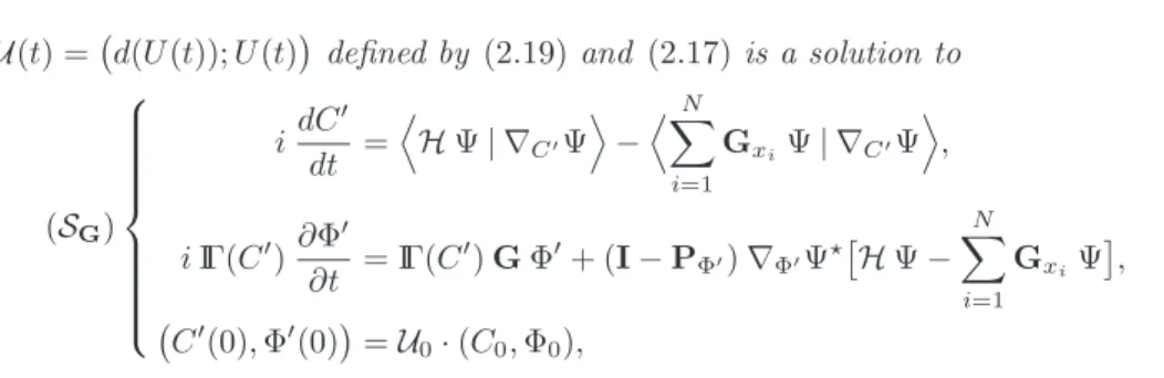
K& that satisfy (3.14) with
U(t) =%d(U (t)); U (t)& defined by (2.19) and (2.17) is a solution to (SG) idC & dt = 6 H Ψ | ∇C!Ψ 7 −6 N ! i=1 GxiΨ| ∇C!Ψ 7 ,
i IΓ(C&)∂Φ&
∂t = IΓ(C &) G Φ&+ (I− P Φ!)∇ Φ!Ψ#,H Ψ − N ! i=1 GxiΨ-,
%C&(0), Φ&(0)& = U
0· (C0, Φ0),
with Ψ = π(C, Φ) = π(C&, Φ&), U0=%U0, d(U0)& ∈ OrK being defined by (2.19) and
with M being the r× r Hermitian matrix given by (3.16).
Remark 3.14. Passing fromS0 toSG amounts to change the operatorH by H −
*N
i=1Gxi in both equations and by adding the linear term IΓ(C&)GΦ&in the equation
satisfied by Φ&. Note that whereas solutions toS
0 in ∂FN,K satisfy
i< ∂φi
∂t ; φj= = 0, for all 1≤ i, j ≤ K, solutions to (SG) satisfy
(3.22) i< ∂φ&i
∂t ; φ
&
j= = <G φ&i; φ&j=.
The system SG corresponds to the choice of the gauge G .
This is illustrated and and summarized on Figure 1 below.
Theorem 3.13 and Lemma 3.11 provide with the differential equation that satis-fies the unitary matrix U (t) that transformsS0intoSG. A direct calculation shows
that, given two self-adjoint one-particle operators G and G&, the solution to
(3.23) i dU dt = U MG→G!, U (t = 0) = U0 with1MG→G! 2 ij =<(G−G &)φ
i; φj= maps a solution to SGto a solution toSG!. In
particular, if we prove existence of solutions for the systemSGfor some operator G
then we have existence of solutions for any systemSG!. Another immediate though
Figure 1. Flow on the Fiber Bundle
below. It states that for any choice of gauge the constraints on the expansion coefficients and on the orbitals are propagated by the flow and the energy is kept constant since it is the case for the system S0. Also the rank of the first-order
density matrices does not depend on the gauge.
Corollary 3.15 (Gauge transforms and conservation properties). Let T > 0. Let G be a self-adjoint (possibly time-dependent) operator acting on L2(Ω). Assume that
there exists a solution to the system SG on [0, T ] such that rank IΓ%C(t)& = K and
such that the matrix t/→<Gφi; φj=1≤i,j≤K is continuous. Then, for all t∈ [0; T ],
(C(t), Φ(t))∈ ∂FN,K,
and the energy is conserved, that is
E%π(C(t), Φ(t))& = E%π(C(0), Φ(0))&.
In addition, Ψ = π(C, Φ) satisfies the Dirac-Frenkel variational principle (3.1). Proof of Corollary 3.15. By Theorem 3.13 and its remark, if (C, Φ) satisfiesSGwith
initial data in ∂FN,K, there exists a family of unitary transforms U ∈ C1%0, T ; OK&
such that (C, Φ) =U · (C&, Φ&) where (C&, Φ&) satisfiesS0with same initial data. By
Lemma 3.2,S0preservesFN,K, hence so doesSGsince U and U = d(U ) are unitary.
Then, by Lemma 2.5, π(C, Φ) = π(C&, Φ&) = Ψ, and the energy is conserved by the flow since it only depends on Ψ. Eventually Eqn. (3.1) is satisfied since TΨ∂BN,K
only depends on the point Ψ on the basis BN,K and not on the preimages in the
fiber π−1(Ψ). !
So far we have considered a generic HamiltonianH and we have written down an abstract coupled system of evolution equations for this operator. In the following subsection we turn to the particular physical case of N -body Schr¨odinger-type operators with pairwise interactions
3.4. N -body Schr¨odinger type operators with pairwise interactions. At this point, we consider an Hamiltonian in L2(ΩN) of the following form
(3.24) HN Ψ = N ! i=1 HxiΨ + ! 1≤i<j≤N v(|xi− xj|) Ψ.
In the above definition, H is a self-adjoint operator acting on L2(Ω). To fix ideas
we take H =−1
2∆ + U . v is a real-valued potential, and we denote
V = !
1≤i<j≤N
v(|xi− xj|) .
Expanding the expression of H in the system S0 and arguing as in the proof of
Theorem 3.13 we obtain (3.25) S0: i dC dt = 6!N i=1 HxiΨ| ∇CΨ 7 +6V Ψ| ∇CΨ 7 i IΓ(C) ∂Φ ∂t = (I− PΦ)∇ΦΨ #?V Ψ + N ! i=1 HxiΨ @ %C(0), Φ(0)& = %C0, Φ0& ∈ FN,K.
Comparing with SystemSGin Theorem 3.13, one observes that the choice of gauge
G = H leads to the equivalent system
(3.26) SH: i dC dt = A V Ψ | ∇CΨ B , i IΓ(C) ∂Φ ∂t = IΓ(C) H Φ + (I− PΦ)∇ΦΨ #[V Ψ] %C(0), Φ(0)& = %C0, Φ0& ∈ FN,K,
(provided t /→ (Hφi; φj) makes sense). From Corollary 3.15 we know that if the
initial data in (3.26) lies inFN,K it persists for all time. This property allows to
recast System (3.26) in a more tractable way where the equations satisfied by the orbitals form a coupled system of non-linear Schr¨odinger-type equations. This new system that it is equivalent to System (3.26) as long as the solution lies in FN,K
will be referred to as working equations following [7, 24]. It is better adapted for well-posedness analysis as will be seen in the forthcoming section.
Proposition 3.16 (Working equations). Let (C, Φ) be a solution to (3.26) inFN,K,
then it is a solution to (3.27) idC dt = K[Φ] C, i IΓ(C)∂Φ ∂t = IΓ(C) H Φ + (I− PΦ) W[C, Φ] Φ, %C(0), Φ(0)& = %C0, Φ0& ∈ F N,K,
where K[Φ] (resp. W[C, Φ]) is a r× r (resp. K × K) Hermitian matrix with entries (3.28) K[Φ]σ,τ= ! i,j∈τ, k,l∈σ δτ\{i,j},σ\{k,l}(−1)τ i,j (−1)σk,lDv%φiφ¯k, ¯φjφl& and (3.29) W[C, Φ] ij(x) = 2 K ! k,l=1 γjkil%φkφ¯l.Ωv)
where here and below we denote Dv(f, g) =
) )
Ω×Ω
v(|x − y|) f(x) g(y) dxdy,
f .Ωv =
)
Ω
v(· − y) f(y) dy
and with the coefficients γijklbeing defined by (2.10) in Proposition 2.3. Conversely,
any solution to (3.27) defines a flow on FN,K as long as IΓ(C) is invertible and is
therefore a solution to (3.26).
Proof. We have to show that for Ψ = π(C, Φ) inBN,K
(3.30) <V Ψ | ∇CΨ= = ∇C<V Ψ | Ψ= = K[Φ] C and (3.31) ∇ΦΨ#[V Ψ] =∇Φ<V Ψ | Ψ= = W[C, Φ] Φ. We start from <V Ψ | Ψ= = ) ) R3×R3 [Ψ⊗ Ψ]:2(x, y, x, y) v(|x − y|) dxdy with [Ψ⊗ Ψ]:2(x, y, x, y) = K ! i,j,k,l=1
according to (2.9). Since only the coefficients γijkl depend on C through Eqn. (2.10) we first get ∇C<V Ψ | Ψ= = K ! i,j,k,l=1
∇C%γijkl& Dv%φiφ¯k, ¯φjφl&.
Hence (3.28) by using again the formula (2.10). We now turn to the proof of (3.31) starting from
<V Ψ | Ψ= = K ! i,j,k,l=1 γijkl ) ) R3×R3
φi(x) φj(y) φk(x) φl(y) v(|x − y|) dxdy.
Then, for every 1≤ p ≤ K ∂ ∂φp <V Ψ | Ψ= = K ! i,j,l=1 γijpl%(φjφl) . v& φi+ K ! i,j,k=1 γijkp%(φiφk) . v& φj = 2 K ! i,j,l=1 γjipl%(φiφl) . v& φj
by interchanging the rˆole played by i and j in the first sum and by using γijkp = γjipk
and renaming k as l in the second one. Comparing with (3.29) we find ∂ ∂φp <V Ψ | Ψ= = 2 K ! j=1 W[C, Φ]pjφj.
To achieve the proof of the proposition we now check that the system of equations in (3.27) preserves FN,K as long as IΓ(C) is invertible. The claim is obvious as
regards the orthonormality of the orbitals since H is self-adjoint and since I− PΦ
projects on Span{Φ}⊥. On the other hand, the equation on the coefficients leads
to d dt"C(t)" 2= 2 8! σ,τ K[Φ]σ,τcτcσ= 0
since the matrix K[Φ] is Hermitian. !
We treat apart in the last two subsections the special cases of the linear free sys-tem with no pairwise interaction and of the time-dependent Hartree–Fock equations for the evolution of a single-determinant (TDHF in short) with pairwise interaction. 3.5. Interactionless Systems v ≡ 0. In this section we consider systems for which the binary interaction potential v is switched off. Then the system (3.26) becomes idC dt = 0, i IΓ(C) ∂Φ ∂t = IΓ(C) H Φ.
From the first equation the coefficients cσ’s are constant during the evolution. In
particular the full-rank assumption is satisfied for all time whenever it is satisfied at start. In that case the orbitals satisfy K independent linear Schr¨odinger equations
(3.32) i∂Φ
and the N -particle wave-function Ψ = π(C, Φ) solves the exact Schr¨odinger equa-tion (3.33) i∂Ψ ∂t = N ! i=1 HxiΨ, Ψ(t = 0) = π(C0, Φ0).
Conversely, the unique solution to the Cauchy problem (3.33) with (C0, Φ0) ∈
∂FN,K coincides with π(C(t), Φ(t)) ∈ FN,K where Φ(t) is the solution to (3.32).
This is a direct consequence of the fact that the linear structure of (3.33) propagates the factorization of a Slater determinant. In particular, this enlightens the fact that the propagation of the full-rank assumption is intricately related to the non-linearities created by the interaction potential v between particles.
3.6. MCTDHF (K = N ) contains TDHF. The TDHF equations write (up to a unitary transform)
(3.34) i∂φi
∂t = H φi+FΦφi,
for 1≤ i ≤ N, with FΦbeing the self-adjoint operator on L2(Ω) that is defined by
FΦw = 1!N j=1 ) Ω v(| · −y|)|φj(y)|2dy 2 w− N ! j=1 1) Ω v(| · −y|)φj(y)w(y) dy 2 φj.
The global-in-time existence of solutions in the energy space H1(ΩN) goes back to
Bove, Da Prato and Fano [6] for bounded interaction potentials and to Chadam and Glassey [12] for the Coulomb potentials. They also checked by integrating the equations that the TDHF equations propagate the orthonormality of the orbitals and that the Hartree–Fock energy is preserved by the flow. Derivation of the TDHF equations from the Dirac-Frenkel variational principle may be encountered in standard Physics textbooks (see e.g. [30]). Let us also mention the work [8] by Canc`es and LeBris who have investigated existence of solutions to TDHF equations including time-dependent electric field and that are coupled with nuclear dynamics.
By simply setting K = N in the MCTDHF formalism one gets (3.35) #ΣN,K = 1 , IΓ(t) = IN
and
Ψ(t) := C(t) φ1(t)∧ . . . ∧ φN(t), C(t) = e−iθΦ(t)
for some θΦ∈ R. In addition according to Remark 2.4,
(3.36) γjkil =
1
2 %δi,jδk,l− δi,kδj,l&. Therefore with the definitions (3.28) and (3.29)
K[Φ] =< V φ1∧ . . . ∧ φN | φ1∧ . . . ∧ φN= = ! i,j,k,l :{i,j}={k,l} (−1)i+pi(j)+k+pk(l)D v(φiφ¯k; ¯φjφl) = N ! i=1 <FΦφi; φi= and N ! j=1 W[C, Φ]ijφj=FΦφi.