Highly resolved global distribution of tropospheric NO₂ using GOME narrow swath mode data

HAL Id: hal-00301165

https://hal.archives-ouvertes.fr/hal-00301165

HAL is a multi-disciplinary open access

archive for the deposit and dissemination of sci-entific research documents, whether they are pub-lished or not. The documents may come from teaching and research institutions in France or abroad, or from public or private research centers.

L’archive ouverte pluridisciplinaire HAL, est destinée au dépôt et à la diffusion de documents scientifiques de niveau recherche, publiés ou non, émanant des établissements d’enseignement et de recherche français ou étrangers, des laboratoires publics ou privés.

Highly resolved global distribution of tropospheric NO2

using GOME narrow swath mode data

S. Beirle, U. Platt, M. Wenig, T. Wagner

To cite this version:

S. Beirle, U. Platt, M. Wenig, T. Wagner. Highly resolved global distribution of tropospheric NO2 using GOME narrow swath mode data. Atmospheric Chemistry and Physics Discussions, European Geosciences Union, 2004, 4 (2), pp.1665-1689. �hal-00301165�

ACPD

Full Screen / Esc

Print Version Interactive Discussion

© EGU 2004

Atmos. Chem. Phys. Discuss., 4, 1665–1689, 2004 www.atmos-chem-phys.org/acpd/4/1665/

SRef-ID: 1680-7375/acpd/2004-4-1665 © European Geosciences Union 2004

Atmospheric Chemistry and Physics Discussions

Highly resolved global distribution of

tropospheric NO

₂

using GOME narrow

swath mode data

S. Beirle1, U. Platt1, M. Wenig2, and T. Wagner1

1

Institut f ¨ur Umweltphysik, Universit ¨at Heidelberg, Germany 2

NASA Goddard Space Flight Center, Greenbelt, MD 20771, USA

Received: 20 January 2004 – Accepted: 16 February 2004 – Published: 16 March 2004 Correspondence to: S. Beirle (beirle@iup.uni-heidelberg.de)

ACPD

Full Screen / Esc

Print Version Interactive Discussion

© EGU 2004 Abstract

The Global Ozone Monitoring Experiment (GOME, since 1995) allows the retrieval of global total column densities of atmospheric trace gases, including NO₂. Tropospheric vertical column densities (VCDs) are derived by estimating the stratospheric fraction from measurements over the remote ocean. Mean maps of tropospheric NO₂ VCDs 5

derived from GOME clearly allow to detect regions with enhanced industrial activity, but the standard spatial resolution of the GOME ground pixels (320×40 km2) is insufficient to resolve regional trace gas distributions or individual cities.

Within the nominal GOME operation, every tenth day measurements in the so called narrow swath mode are executed with a much better spatial resolution (80×40 km2). 10

Though the global coverage of these data is – due to the narrow swath – rather poor, the mean distribution over several years (1997–2001) allows to construct a much more detailed picture of the global NO₂distribution, especially if corrected for seasonal ef-fects. It vividly illustrates the shortcomings of the standard size GOME pixels and reveals an unprecedented wealth of details in the global distribution of tropospheric 15

NO₂. Sharply localised spots of enhanced NO₂ VCD can be associated directly to cities, large power plants, and heavy industry centers.

The long time series of GOME data allows a quantitative comparison of the narrow swath mode data to the nominal resolution that holds general information on the de-pendency of NO₂VCDs on pixel size. This is important for new instruments like SCIA-20

MACHY (launched March 2002 on ENVISAT) or OMI and GOME II (to be launched 2004 and 2005, respectively) with an improved spatial resolution.

1. Introduction

The atmospheric composition has changed dramatically over the last 150 years due to the industrial revolution. Among the various emitted pollutants nitrogen oxides 25

ACPD

Full Screen / Esc

Print Version Interactive Discussion

© EGU 2004

a large impact on human health, climate and atmospheric chemistry, e.g. through their role in catalytic ozone production and their influence on the OH concentration. More-over, the estimation of the strengths of the different NO_x sources (industry, biomass burning, aircraft, soil emissions, lightning) still has high uncertainties (e.g. Lee et al., 1997), with anthropogenic NO_x (fossil fuel combustion) estimated to account for more 5

than 50% of the overall production. Anthropogenic sources are distributed quite inho-mogeneously around the globe and are concentrated in highly populated and industri-alized areas, where NO_x is produced by traffic, power generation, heavy industry and domestic combustion.

Satellite measurements are a powerful tool for monitoring trace gas emissions, since 10

the whole globe is observed with a single instrument over long periods of time. The general features of the global distribution of tropospheric NO₂ have been reported in several studies (Leue et al., 2001; Velders et al., 2001; Wenig, 2001; Richter and Burrows, 2002; Martin et al., 2002) using data from the Global Ozone Monitoring Ex-periment (GOME) on board the ESA satellite ERS-2, launched in April 1995 (Burrows, 15

1999). These studies clearly showed, that satellite observations have the potential to identify different sources of tropospheric NO_x, in particular the industrialized areas of the world (e.g. the USA, central Europe, China). However, the standard spatial reso-lution of one GOME ground pixel (320×40 km2) is insufficient to resolve details of the regional NO₂distribution or individual cities. To improve our knowledge of the distribu-20

tion of NO₂burden, i.e. the location and extent of sources and the role of transport, and to potentiate quantitative estimates of emissions, a better spatial resolution is essential.

2. Retrieval

2.1. Tropospheric NO₂VCD from GOME

The ERS-2 satellite flies along a sun-synchronous polar orbit and crosses the equa-25

ACPD

Full Screen / Esc

Print Version Interactive Discussion

© EGU 2004

radiation reflected by the earth in the UV/vis spectral range (240–790 nm) with a res-olution of about 0.2–0.4 nm. Global coverage at the equator is achieved every three days. Column densities of several trace gases can be determined, applying Differential Optical Absorption Spectroscopy (DOAS) (Platt, 1994). The retrieval of vertical column densities (VCDs) of NO₂is described in detail in Wagner (1999) and Leue et al. (2001). 5

Since the global distribution of stratospheric NO₂ is much more homogeneous in space and time than in the troposphere, it is possible to estimate the stratospheric fraction of the total column (e.g. Leue et al., 2001; Velders et al., 2001; Wenig, 2001). Systematic errors in the total column due to the degradation of the GOME instrument or the diffuser plate (Richter and Wagner, 2001) are included in the stratospheric es-10

timation, and thus will not affect the resulting tropospheric column. For this study, the latitude dependent stratospheric column of NO₂was determined in a reference sector over the remote Pacific (Richter and Burrows, 2002). The difference between the total and the stratospheric column represents the tropospheric fraction. For a quantitative analysis these values have to be corrected for the reduced sensitivity of GOME towards 15

tropospheric trace gases. The absolute value of the correction factor depends on trace gas profile, earth albedo, cloud fraction and aerosol load (Leue et al., 2001; Wagner et al., 2001 (BrO); Richter and Burrows, 2002; Martin et al., 2003). In this study, we apply a uniform correction factor of 2, to keep the analysis as elementary as possible and to avoid uncertainties emerging from external data. The actual column is probably 20

higher due to the shielding effect of clouds (Richter and Burrows, 2002; Wagner et al., 2003). However, we do not correct for the cloud fraction, since its influence is not fully understood (see below) and differs regionally (Wenig, 2001).

2.2. GOME spatial resolution and narrow swath mode

GOME scans the Earth’s surface by moving the scan mirror by ±31◦, corresponding 25

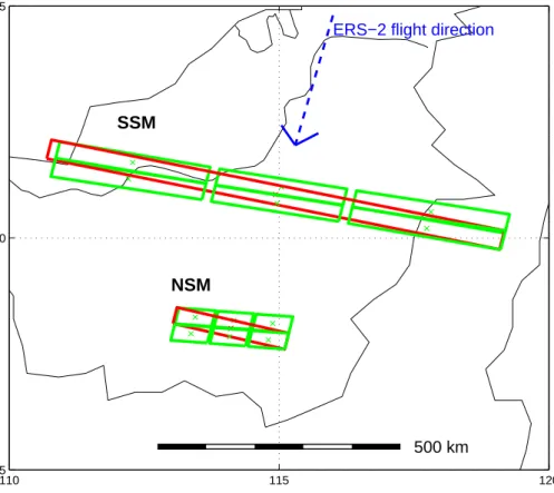
to a cross track swath width of 960 km. During each scan, three ground pixels are mapped with a spatial resolution of 320 km east-west and 40 km north-south, followed by one backscan pixel with an extent of 960×40 km2(see Fig. 1).

ACPD

Full Screen / Esc

Print Version Interactive Discussion

© EGU 2004

Besides this standard size mode (referred as SSM below), GOME has the possibility to reduce the range of the scan mirror angle. This is done since end of June 1997: an angular range of ±8.7◦is applied three days a month, namely the 4th/5th, the 14th/15th and the 24th/25th of every month between the sun calibrations of those days. These measurements in the so called narrow swath mode (referred as NSM below) have a 5

spatial resolution of 80×40 km2 (forward scan) and 240×40 km2 (backscan), respec-tively (see Fig. 1). Additional information on the GOME viewing geometry is described in the GOME users manual (Bednarz, 1995).

The NSM improves the spatial resolution, but the global coverage is reduced: in the SSM GOME reaches global coverage each 3 days, while for the NSM 12 measurement 10

days are required. Since the NSM is only applied every 10th day, statistically 120 days are needed to reach a global cover with the NSM orbits. Figure 2 shows the total number of measurements in the NSM during the 5 year period from 1997 to 2001 around the globe.

2.3. High quality map from high resolution NSM data 15

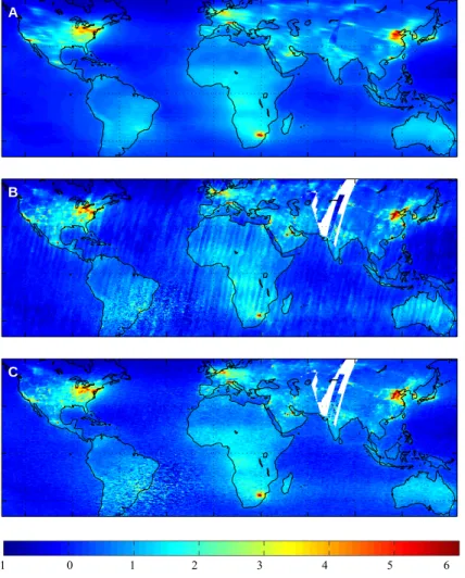
Figure 3a shows a global map of the mean tropospheric NO₂ VCD, using the SSM (320 km by 40 km) GOME pixels 1996–2001 (no backscans). Regions of industrial activity show significantly enhanced VCDs. Also the influence of biomass burning and high lightning activity is detectable (e.g. Leue et al., 2001; Richter and Burrows, 2002; Beirle et al., 2003). However, the emissions of comparably small sources like single 20

cities are “smeared out” due to the large east-west extension of the GOME ground pixels.

Figure 3b depicts the mean tropospheric NO₂ VCD of all NSM pixels during 1997– 2001. The better spatial resolution reveals many more details of the global distribution of tropospheric NO₂. But whereas Fig. 3a shows a quite smooth distribution, Fig. 3b 25

exhibits stripe like patterns parallel to the ERS-2 flight direction.

The reason for these stripes is the sparse global coverage. In the NSM, each point on the Earth is scanned only about 10-15 times during a six year time period (Fig. 2).

ACPD

Full Screen / Esc

Print Version Interactive Discussion

© EGU 2004

Moreover, these measurements are not distributed homogeneously over the year. Es-pecially for regions where the NO₂ burden varies with season (e.g. due to biomass burning), the actual date of the measurement becomes essential. This is illustrated in Fig. 4 for the case of Central Africa, a region with yearly biomass burning events from June to September. Two neighbouring locations are selected, showing (A) a high 5

and (B) a quite low tropospheric NO₂ VCD. In Table 1, the dates of measurements in the NSM are listed for both locations. Whereas all (but one) scans of location A were made during the burning season, only one out of thirteen scans took place in the burn-ing season for location B. So the main reason for the stripe structure is the fact that the local measurements are not distributed uniformly throughout the year. Therefore we 10

call it the “seasonal effect”, since the measured NO₂ VCD depends on the season in which the majority of the measurements were made.

Seasonal variations should not be influencing a multi-year average. The stripe struc-ture could be reduced by spatially smoothing the data. However, it is the whole idea of this investigation to obtain a map of the NO₂ distribution with improved resolution 15

from the NSM data. Therefore, to account for the patchy temporal coverage, we ap-ply a more sophisticated correction of the seasonal effect. For this procedure we use our knowledge of the mean distribution of NO₂VCD from the SSM as seen in Fig. 3a: Each GOME measurement consists of three forward scan pixels and a subsequent backscan pixel (see Fig. 1). The spatial resolution (240×40 km2) of the backscan pixel 20

in the NSM is quite comparable to the extent of the SSM forward scan pixels. Hence we can estimate the seasonal offset for each individual NSM measurement by comparing the NSM backscan VCD with the mean of all SSM pixels at the same location, and correct the NSM forward scan pixels by this “offset”.

The resulting seasonally corrected mean tropospheric NO₂ VCD distribution of the 25

NSM pixels is shown in Fig. 3c, which is free of the stripelike structures of Fig. 3a. The remaining noisy values around South America are due to the South Atlantic anomaly (Heirtzler, 2002).

ACPD

Full Screen / Esc

Print Version Interactive Discussion

© EGU 2004 3. Global distribution of tropospheric NO₂

Figure 3c reveals many details on the tropospheric NO₂ distribution. In the polluted areas in North America, Europe, the Middle East and Far East, structures can be seen with unprecedented spatial resolution. Many “hot spots” show up, and sources of NO₂ can be clearly localized and identified (mostly large cities). Even the highly populated 5

Nile river valley in Egypt is visible. On the other hand, tropical regions of enhanced NO₂ VCD like Congo show no new spatial information, since the sources (biomass burning, lightning) are not sharply localized in the mean taken over several years.

To illustrate the new insight in the tropospheric NO₂ distribution from NSM data in detail, Fig. 5 displays zooms of Fig. 3c for (a) North America and (b) Europe as exam-10

ples. Additionally, the location of larger cities is marked, and in (b) contour lines (1 km altitude) indicate mountains.

In the USA, nearly each major city can be associated directly to a NO₂-“hot spot” in Fig. 5a, and vice versa. Nevertheless, there also is a significant area of elevated NO₂ in a remote region (marked white in Fig. 5a). This is due to a field of large coal 15

power plants (e.g. “Four Corners” with a capacity of 2 GW, see referenced weblinks). The spot in North Mexico (marked grey) is associated with coal power plants as well (“Carbon 1/2”, Piedras Negras).

Also in Europe, the NO₂ load generally reflects human activity. Major cities (e.g. Moscow, Madrid, Istanbul or London) show enhanced levels of NO₂, like in the USA. 20

However, there are also some cities with more than 1 million inhabitants (e.g. Rome, Berlin, Warsaw), that show rather low levels of NO₂, while the highest levels of NO₂ are found in some industrial areas (Po Valley, Ruhr area). These data might help to quantify the different anthropogenic sources (traffic via industry) separately.

ACPD

Full Screen / Esc

Print Version Interactive Discussion

© EGU 2004 4. Extent of NO₂pollution “hot spots”

Though the number of available NSM observations for each given location is rather small (see Fig. 2), the “hot spots” detected round the globe are rich in contrast and have well defined edges. Apart from congested areas like the US Eastcoast, western Europe or east China, where large regions show enhanced NO₂levels, there are several NO₂ 5

peaks according to large cities that are comparable in their spatial extent (see Fig. 3c). The Istanbul plume, as a typical example, ranges approx. 80 km in east-west (i.e. the width of the NSM!) and 50 km in north-south-direction (the higher east-west-extent is likely to reflect the GOME ground pixel geometry). Less than 80km aside from the plume center the NO₂VCD is already on the normal background level. Therefore, only 10

the tracks directly crossing the source see an enhanced NO₂VCD.

4.1. Lifetime of boundary layer NO_x

The low spatial extent of the hot spots and the sharp decrease of NO₂ VCD at their edges indicate that the average lifetime of NO_xin the lower troposphere must be rather small. To give a rough quantitative estimation, we assume a first order, i.e. exponential 15

loss of NO_x with a constant lifetime τ throughout the year. In a distance of approx. 60 km the VCD is dropped to 1/e. The distance is related to the time via x=vτ, with v being the mean wind speed. For v=1 m/s (as a lower limit) this results in a mean lifetime of about τ=60 km/1 (m/s) ≈17 h, and less for higher mean wind speeds. Although this is a very rough estimation, the mean lifetime of NO₂in the boundary layer obviously can 20

not be much larger than a day, since otherwise an offwind plume should be detectable in the NSM data. So NSM GOME observations allow to derive an upper limit to the lifetime of boundary layer NO₂, and thus NO_x, for sites around the globe. (Beirle et al., 2003, used GOME data to estimate the NO_x lifetime of 6 h in summer and 24–36 h in winter for Germany).

ACPD

Full Screen / Esc

Print Version Interactive Discussion

© EGU 2004

4.2. NSM via SSM resolution

In the SSM, pollution peaks are obviously “smeared out” due to the 320 km width of the GOME pixel in west-east-direction (see Fig. 3a; compare, for instance, the shape of the Hong Kong peak in 3a and 3c). For the same reason the maximal VCDs measured in the SSM are lower than in the NSM. A quantitative estimation of this effect is illustrated 5

in Fig. 6: A given (Gaussian) distribution of NO₂pollution with a FWHM of 20, 50, 100 or 200 km (i.e. the extent of large cities or congested areas) is scanned with pixels of NSM and SSM size respectively. The actual VCD is drastically underestimated by SSM observations at its peak, but overestimated at its edges. This effect is much weaker for the NSM, since its resolution approaches the actual extent of the NO₂ distribution. 10

Figure 6 also displays the ratio of the modelled maxima in the NSM and the SSM, which was found to be close to 4 for a point source and approaches unity for extended sources. Table 2 now lists the actual measured NO₂VCDs over some selected cities for the NSM and the SSM. As expected, the NSM observations show higher VCDs. A comparison of the measured NSM/SSM ratios in Table 2 with those calculated in Fig. 6 15

also allows to deduce the spatial extent of the sources. Mexico city, for instance, where the NSM/SSM-ratio is 3.2, can be regarded as an isolated source spot with an extent of <80 km. The Ruhr Area, on the other hand, where the NSM/SSM ratio is only 1.46, has a large extent and is probably also affected by sources in the Netherlands and Belgium.

20

To further analyse the “smoothing effect” for SSM measurements, we plotted the difference of the NSM forwardscans (i.e. high resolution observations), and the NSM backscans (representing nearly the SSM resolution), in Fig. 7 (for the same clippings as in Fig. 5). The dipolar structure indicated in Fig. 6 (i.e. the underestimation of the SSM observations above the spot and underestimation left and right) is impressively 25

illustrated in Fig. 7, especially for isolated cities (Mexico City, Madrid, Salt Lake City, Phoenix) and cities with very high NO₂ VCDs (Los Angeles). This plot indicates the location and the extent of sources even better than Fig. 5, especially for “hot spots”

ACPD

Full Screen / Esc

Print Version Interactive Discussion

© EGU 2004

in polluted regions. The Po valley, for instance, is generally highly polluted by Milan emissions. Figure 7, however, reveals that there are at least two more hot spots, namely Turin and Padua/Venice.

Furthermore, Fig. 7 clearly displays locations where the SSM GOME observations overestimate the actual burden due to the ”smearing out” of local peaks. This is a 5

valuable additional information for the interpretation of GOME studies. For instance, the mean of the SSM GOME pixels (Fig. 3a) shows enhanced VCD of NO₂ over the North Sea between England and the Netherlands. Figure 7 shows that these VCDs are overestimated. So, the observed enhancement is not only due to transport by wind as may be assumed, but also to the fact that each nominal pixel in this area either covers 10

polluted sites in England (Manchester, Sheffield etc.) or the Netherlands (Rotterdam). The VCD over the western Alpine mountains is also drastically overestimated by the SSM observations due to the short distance to Milan.

5. Influence of the cloud fraction on the mean VCD

Boundary layer NO₂ may be shielded by clouds. Due to the high cloud albedo, this 15

effect is nonlinear: the average of two half clouded pixel results in a VCD different from the mean of one cloud free and one totally clouded pixel (e.g. Wenig, 2001; Richter and Burrows, 2002; see also Fig. 8).

Since the NSM is sampled with a 4 times higher spatial resolution, those pixels are more often cloud free than SSM pixels: For the US, for instance, the percentage of 20

cloud free (i.e. having cloud fraction below 10%) pixels is 34.7% in the SSM and 40.7% in the NSM (Cloud fraction taken from the HICRU database, Grzegorski, 2003).There-fore (and for the a2003).There-forementioned reason) we would expect the NSM forwardscan ob-servations to yield generally higher VCDs than SSM or NSM backscans respectively.

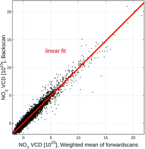
To analyse this effect, in Fig. 9 we compared the NSM backscan with the weighted 25

average of the respective forwardscans that it covers.

ACPD

Full Screen / Esc

Print Version Interactive Discussion

© EGU 2004

means that in contrast to our expectation the pixel size has almost no influence on

the mean NO₂ VCD. Partly, this could be explained by a significant amount of NO₂ above the clouds (Wenig, 2001; Richter and Burrows, 2002). On the other hand, it is obvious, that in many polluted regions the tropospheric NO_x is close to the ground. At present, we do not understand our findings and intend to present a detailed analysis 5

of the dependency of cloud fraction distributions on pixel size and the relating radiative transfer aspects in a future study. However, our finding has a high relevance on the quantitative interpretation of the results of GOME and its successors like SCIAMACHY, OMI or GOME II.

6. Conclusion and outlook

10

The analysis of the GOME observations in the narrow swath mode results in a global map of tropospheric NO₂with an unmatched spatial resolution (80×40 km2). The com-parison of forward- and backscans allows to correct for data fluctuations due to the patchy temporal sampling.

The resulting maps (Figs. 3c, 5 and 6) display many “hot spots” which are not visible 15

in the standard GOME observations. Most hot spots can directly be associated with cities. But, even large power plants like “Four Corners” in the USA can be detected. This demonstrates that satellite instruments are capable of detecting and monitoring local pollution and provide valuable additional information on the global distribution of NO_x sources which might be used for comparison and improvement of emission data 20

bases. The quite sharply localised hot spots also indicate a low lifetime of boundary layer NO_x of less than one day, even for cities like Moscow at 56◦N.

The problem of poor temporal coverage of the GOME measurements in the narrow swath mode will be resolved by SCIAMACHY (currently in its validation phase) with an even better spatial resolution (60×30 km2) and further satellite missions (OMI, GOME 25

II).

ACPD

Full Screen / Esc

Print Version Interactive Discussion

© EGU 2004

in size to the SSM) observations reveals that the pixel size has nearly no effect on themean NO₂ VCD. This is quite surprising, since the pixel size definitely affects the distribution of fractional cloud fraction. This finding has important consequences on the quantitative interpretation of SCIAMACHY and OMI data (and possible comparisons to GOME).

5

Acknowledgements. This study was funded by the German Ministry for Education and

Re-search as part of the NOXTRAM project (Atmospheric ReRe-search 2000). We like to thank the European Space Agency (ESA) operation center in Frascati (Italy) and the “Deutsches Zentrum f ¨ur Luft- und Raumfahrt” DLR (Germany) for providing the ERS-2 satellite data. Cloud data was taken from the HICRU data base provided by M. Grzegorski.

10

Edited by: A. Richter

References

Bednarz, F.: Global Ozone Monitoring Experiment (GOME) Users Manual, Eur. Space Agency Publ. Div., Noordwijk, The Netherlands, 1995.

15

Beirle, S., Platt, U., Wenig, M., and Wagner, T.: Weekly cycle of NO₂by GOME measurements: a signature of anthropogenic sources, Atmos. Chem. Phys. 3, 2225–2232, 2003.

Beirle, S., Platt, U., Wenig, M., and Wagner, T.: NOx production by lightning estimated with GOME, Adv. Space Res., accepted, 2003.

Burrows, J., Weber, M., Buchwitz, M., Rozanov, V., Ladstetter-Weienmayer, A., Richter, A., De 20

Beek, R., Hoogen, R., Bramstedt, K., Eichmann, K. U. , Eisinger, M., and Perner, D.: The Global Ozone Monitoring Experiment (GOME): Mission concept and first scientific results, J. Atmos. Sci., 56, 151–175, 1999.

Four Corners Power Plant:http://www.srpnet.com/power/stations/fourcorners.asp;http://www.

pnm.com/systems/4c.htm. 25

Grzegorski, M.: Determination of cloud parameters for the Global Ozone Monitoring Experi-ment with broad band spectrometers and from absorption bands of oxygen dimer, Diploma thesis, University of Heidelberg, Germany, 2003.

ACPD

Full Screen / Esc

Print Version Interactive Discussion

© EGU 2004

Heirtzler, J.: The future of the South Atlantic anomaly and implications for radiation damage in space, J. Atmos. Solar-Terr. Phys., 64, 1701–1708, 2002.

Lee, D. S., K ¨ohler, I., Grobler, E., Rohrer, F., Sausen, R., Gallardo-Klenner, L., Olivier, J. G. J., Dentener, F. J., and Bouwman, A. F.: Estimations of global NO_x emissions and their uncertainties, Atmos. Environ., 31, 1735–1749, 1997.

5

Leue, C., Wenig, M., Wagner, T., Klimm, O., Platt, U., and J ¨ahne, B.: Quantitative analysis of NO₂emissions from GOME satellite image sequences, J. Geophys. Res., 106, 5493–5505, 2001.

Martin, R. V., Chance, K., Jacob, D. J., Kurosu, T. P., Spurr, R. J. D., Bucsela, E., Gleason, J. F., Palmer, P. I., Bey, I., Fiore, A. M., Li, Q., Yantosca, R. M., and Koelemeijer, R. B. A.: An 10

improved retrieval of tropospheric nitrogen dioxide from GOME, J. Geophys. Res., 107, D20, 4437, doi:10.1029/2001JD001027, 2002.

Martin, R. V., Jacob, D. J., Chance, K., Kurosu, T. P., Palmer, P. I., Evans, M. J.: Global inventory of nitrogen oxide emissions constrained by space-based observations of NO₂ columns, J. Geophys. Res., 108, 4537, doi:10.1029/2003JD003453, 2003.

15

Platt, U.: Differential optical absorption spectroscopy (DOAS), in Air Monitoring by Spectromet-ric Techniques, edited by Sigrist, M., Chemical Analysis Series, 127, 27–84, John Wilsy, New York, 1994.

Richter, A. and Wagner, T.: Diffuser Plate Spectral Structures and their Influence on GOME Slant Columns, Technical Note,http://giger.iup.uni-heidelberg.de/thomas/diffuser gome.pdf, 20

January 2001.

Richter A. and Burrows, J.: Retrieval of Tropospheric NO₂ from GOME Measurements, Adv. Space Res., 29, 11, 1673–1683, 2002.

Velders, G.J.M., Granier, C., Portmann, R.W., Pfeilsticker, K., Wenig, M., Wagner, T., Platt, U., Richter, A., and Burrows, J.: Global tropospheric NO₂column distributions: Comparing 25

3-D model calculations with GOME measurements, J. Geophys. Res., 106, 12 643–12 660, 2001.

Wagner, T.: Satellite observations of atmospheric halogen oxides, Ph.D. thesis, University of Heidelberg, Germany, 1999.

Wagner, T., Leue, C., Wenig, M., Pfeilsticker, K., and Platt, U.: Spatial and temporal distribution 30

of enhanced boundary layer BrO concentrations measured by the GOME instrument aboard ERS-2, J. Geophys. Res., 106, 24 225–24 236, 2001a.

In-ACPD

Full Screen / Esc

Print Version Interactive Discussion

© EGU 2004

vestigation of Cloud Sensitive Parameters as Measured by GOME, TROPOSAT final report, Sounding the Troposphere from Space: a New Era for Atmospheric Chemistry, Springer, Berlin, 199–210, 2003.

Wenig, M.: Satellite Measurements of Long-Term Global Tropospheric Trace Gas Distributions and Source Strengths, Ph.D. thesis, University of Heidelberg, Germany,http://mark-wenig.

5

ACPD

Full Screen / Esc

Print Version Interactive Discussion

© EGU 2004

Table 1. Dates of measurements for the sites marked in Fig. 4. Bold typing indicates the burning season in Central Africa (June–September).

Site A Site B 05.09.1997 15.03.1998 25.09.1998 05.05.1998 05.07.1999 05.01.1999 25.08.1999 25.02.1999 25.10.1999 25.05.1999 25.08.2000 15.07.1999 25.07.2001 05.12.1999 25.01.2000 25.05.2000 15.10.2000 05.12.2000 05.04.2001 25.12.2001

ACPD

Full Screen / Esc

Print Version Interactive Discussion

© EGU 2004

Table 2. Comparison of NSM and SSM mean tropospheric NO₂ VCD (1015molec/cm2) for different cities/regions. The third column gives the ratio NSM/SSM, that is compared with the simulations in Fig. 7. City/region VCD SSM VCD NSM Ratio NSM/SSM Los Angeles 8.70 22.42 2.58 Phoenix 3.72 7.54 2.03 New York 4.98 8.30 1.67 Mexico City 4.88 15.66 3.21 Ruhr Area 3.94 5.74 1.46 Milan 5.68 8.30 1.46 South Africa 6.56 9.22 1.41 Dschidda 3.18 8.44 2.65 Rijad 4.32 9.68 2.24 Hongkong 6.16 12.86 2.09 Shanghai 4.32 7.84 1.81 Beijing 5.70 8.32 1.46 Seoul 5.46 10.24 1.88 Tokio 4.30 8.74 2.03 Istanbul 2.44 5.56 2.28

ACPD

Full Screen / Esc

Print Version Interactive Discussion © EGU 2004 110 115 120 −5 0 5 500 km

ERS−2 flight direction

SSM

NSM

Fig. 1. Spatial extension and geometry of the GOME ground pixels. A snapshot of the standard

size mode (SSM, 320×40 km2) and the narrow swath mode (NSM, 80×40 km2) is shown at the equator (Borneo). The forward scan pixels are green, the subsequent backscans, having triple length, red.

ACPD

Full Screen / Esc

Print Version Interactive Discussion

© EGU 2004

Figure 1: Spatial extension and geometry of the GOME ground pixels. A snapshots of the standard size mode (SSM, 320*40 km2) and the narrow swath mode (NSM, 80*40 km2) is shown at the equator (Borneo). The forward scan pixels are green, the subsequent backscans, having triple length, red.

Figure 2: Total number of GOME scans in the narrow swath mode (NSM) 1997-2001.

10

ACPD

Full Screen / Esc

Print Version Interactive Discussion © EGU 2004 A B C a) b) c) -1 0 1 2 3 4 5 6 Figure 3: Global mean of tropospheric NO2 VCD (1015 molecules/cm2), using a) all nominal

pixels 1996-2001 (no backscans), b) NSM pixels only 1997-2001, c) NSM pixels only (1997-2001), corrected for seasonal effects.

Fig. 3. Global mean of tropospheric NO₂VCD (1015molecules/cm2), using(a) all nominal pixels

1996–2001 (no backscans),(b) NSM pixels only 1997–2001, (c) NSM pixels only (1997–2001),

corrected for seasonal effects.

ACPD

Full Screen / Esc

Print Version Interactive Discussion

© EGU 2004

Figure 4: Zoom of Fig. 2b on Central Africa to explain the stripe like features. Two

neighbouring sites with high (A) and low (B) VCD of tropospheric NO

2

are compared. Table

1 reveals that for site (A) almost all (whereas for site (B) only 1) measurements took place

during the burning season.

12

Fig. 4. Zoom of Fig. 3b on Central Africa to explain the stripe like features. Two neighbouring

sites with high (A) and low (B) VCD of tropospheric NO₂ are compared. Table 1 reveals that for site (A) almost all (whereas for site (B) only 1) measurements took place during the burning season.

ACPD

Full Screen / Esc

Print Version Interactive Discussion

© EGU 2004

Figure 5: Zoom of Fig. 3c for North America (a) and Europe (b). Cities with more than 200000 (a) and 500000

(b) inhabitants are marked (cities within a 100 km distance are cumulated). The marked spots in (a) indicate NO2

pollution that does not coincide with a large city, but instead with large coal fired power plants (“Four Corners”, USA (white); “Piedras Negras”, Mexico (grey)). For Europe, also the 1 km altitude contour lines are shown illustrating mountains. The projections are equal-area for 35°N (a) and 45°N (b), respectively.

13

Fig. 5. Zoom of Fig. 3c for North America (a) and Europe (b). Cities with more than 200000 (a)

and 500 000 (b) inhabitants are marked (cities within a 100 km distance are cumulated). The marked spots in (a) indicate NO₂pollution that does not coincide with a large city, but instead with large coal fired power plants (“Four Corners”, USA (white); “Piedras Negras”, Mexico (grey)). For Europe, also the 1 km altitude contour lines are shown illustrating mountains. The projections are equal-area for 35◦N (a) and 45◦N (b), respectively.

ACPD

Full Screen / Esc

Print Version Interactive Discussion

© EGU 2004

Figure 6: Illustration of the smoothing effect of the GOME SSM pixels. A given pollution distribution (black), assumed to be Gaussian with different FWHM, is underestimated by GOME SSM (blue) over its maximum, but overestimated over its edges. This effect is much weaker for the NSM (red).

The dotted boxes indicate an individual measurement where the middle GOME pixel is centered at the pollution peak; the solid lines display the mean of a large number of measurements at different positions, i.e. the actual pollution distribution convoluted with the GOME resolution. The numbers give the ratio of the measured maximum in the NSM and the SSM.

Fig. 6. Illustration of the smoothing effect of the GOME SSM pixels. A given pollution

distribu-tion (black), assumed to be Gaussian with different FWHM, is underestimated by GOME SSM (blue) over its maximum, but overestimated over its edges. This effect is much weaker for the NSM (red). The dotted boxes indicate an individual measurement where the middle GOME pixel is centered at the pollution peak; the solid lines display the mean of a large number of measurements at different positions, i.e. the actual pollution distribution convoluted with the GOME resolution. The numbers give the ratio of the measured maximum in the NSM and the SSM.

ACPD

Full Screen / Esc

Print Version Interactive Discussion

© EGU 2004

Figure 7: Difference of the NSM forward- and backscan pixels (1015 _molec/cm2_{) for North} America (a) and Europe (b). Red spots show locations, where the tropospheric NO2 column is underestimated by the nominal viewing pixels from GOME (several cities), whereas it is overestimated for the blue spots (e.g. the Alpine mountains).

15 −2.5 −2 −1.5 −1 −0.5 0 0.5 1 1.5 2 2.5 0.5 0.6 0.7 0.8 0.9 1 1.1 1.2 1.3 1.4 1.5 0.5 0.6 0.7 0.8 0.9 1 1.1 1.2 1.3 1.4 1.5

Fig. 7. Difference of the NSM forward- and backscan pixels (1015molec/cm2) for North America

(a) and Europe (b). Red spots show locations, where the tropospheric NO₂column is underes-timated by the nominal viewing pixels from GOME (several cities), whereas it is overesunderes-timated for the blue spots (e.g. the Alpine mountains).

ACPD

Full Screen / Esc

Print Version Interactive Discussion

© EGU 2004

Figure 8: Shielding effect of clouds

For a cloudy scene, boundary layer NO

2

would be shielded and thus be „invisible“ for

GOME. Furthermore, since the cloud albedo is much higher than the ground albedo, the

observed light comes predominantly from the clouds, leading to a further underestimation of

boundary layer NO

2

.

For instance, in the given scene with 50% cloud cover the reflected light intensity would be

0.5*I*0.8 + 0.5*I*0.05=(0.4+0.025)*I. I.e., only 6% of the measured light comes from the

ground, i.e. has crossed the NO

2

profile. Therefore, in the backscan only 6% of the actual NO

2

column would be detected.

In the NSM forward scans there would be one totally cloudy pixel (seeing no NO

2

), one pixel

with 50% cloud cover (seeing 6% as for the backsacn) and one cloud free pixel (seeing 100%

of the actual NO

2

column!). In average, the NSM forward scans would detect

(0+0.06+1)/3=35% of the boundary layer NO

2

, i.e. 6 times as much as for the backscan

observation!

16

Fig. 8. Shielding effect of clouds For a cloudy scene, boundary layer NO₂would be shielded and thus be “invisible” for GOME. Furthermore, since the cloud albedo is much higher than the ground albedo, the observed light comes predominantly from the clouds, leading to a further underestimation of boundary layer NO₂. For instance, in the given scene with 50% cloud fraction the reflected light intensity would be 0.5×I×0.8+0.5×I×0.05=(0.4+0.025)×I. I.e. only 6% of the measured light comes from the ground, i.e. has crossed the NO₂profile. Therefore, in the backscan only 6% of the actual NO₂column would be detected. In the NSM forward scans there would be one totally cloudy pixel (seeing no NO2), one pixel with 50% cloud fraction (seeing 6% as for the backscan) and one cloud free pixel (seeing 100% of the actual NO2 column!). In average, the NSM forward scans would detect (0+0.06+1)/3=35% of the boundary layer NO₂, i.e. 6 times as much as for the backscan observation!

ACPD

Full Screen / Esc

Print Version Interactive Discussion © EGU 2004 0 5 10 15 20 0 5 10 15 20

NO

VCD [10

], Weighted mean of forwardscans

NO

VCD [10

], Backscan

linear fit

Fig. 9. Correlation of the mean NO₂ VCD of the NSM forwardscans and the respective backscan (all NSM observations over the US, Europe, China and Japan). The slope of the linear fit is 0.98.