Direct observation of two dimensional trace gas distribution with an airborne Imaging DOAS instrument

(1)

HAL Id: hal-00304268

https://hal.archives-ouvertes.fr/hal-00304268

Submitted on 13 Jun 2008

HAL is a multi-disciplinary open access

archive for the deposit and dissemination of sci-entific research documents, whether they are pub-lished or not. The documents may come from teaching and research institutions in France or abroad, or from public or private research centers.

L’archive ouverte pluridisciplinaire HAL, est destinée au dépôt et à la diffusion de documents scientifiques de niveau recherche, publiés ou non, émanant des établissements d’enseignement et de recherche français ou étrangers, des laboratoires publics ou privés.

Direct observation of two dimensional trace gas

distribution with an airborne Imaging DOAS instrument

K.-P. Heue, T. Wagner, S. P. Broccardo, D. Walter, S. J. Piketh, K. E. Ross,

S. Beirle, U. Platt

To cite this version:

K.-P. Heue, T. Wagner, S. P. Broccardo, D. Walter, S. J. Piketh, et al.. Direct observation of two di-mensional trace gas distribution with an airborne Imaging DOAS instrument. Atmospheric Chemistry and Physics Discussions, European Geosciences Union, 2008, 8 (3), pp.11879-11907. �hal-00304268�

(2)

ACPD

8, 11879–11907, 2008 Airborne imaging DOAS K.-P. Heue et al. Title Page Abstract Introduction Conclusions References Tables Figures ◭ ◮ ◭ ◮ Back Close

Full Screen / Esc

Printer-friendly Version

Interactive Discussion Atmos. Chem. Phys. Discuss., 8, 11879–11907, 2008

www.atmos-chem-phys-discuss.net/8/11879/2008/ © Author(s) 2008. This work is distributed under the Creative Commons Attribution 3.0 License.

Atmospheric Chemistry and Physics Discussions

Direct observation of two dimensional

trace gas distribution with an airborne

Imaging DOAS instrument

K.-P. Heue1, T. Wagner2, S. P. Broccardo3, D. Walter1, S. J. Piketh3, K. E. Ross4, S. Beirle2, and U. Platt1

1

Institut f ¨ur Umweltphysik (IUP), Universit ¨at Heidelberg, Heidelberg, Germany 2

Max Planck Institut f ¨ur Chemie, Mainz, Germany 3

Climatology Research Group, University of the Witwatersrand, Johannesburg, South Africa 4

Research and Innovation Department, Eskom, South Africa

Received: 26 March 2008 – Accepted: 30 May 2008 – Published: 13 June 2008 Correspondence to: K.-P. Heue (klaus-peter.heue@iup.uni-heidelberg.de)

(3)

ACPD

Full Screen / Esc

Interactive Discussion

Abstract

In many investigations of tropospheric chemistry information about the two dimensional distribution of trace gases on a small scale (e.g. tens to hundreds of meters) is highly desirable. An airborne instrument based on imaging Differential Optical Absorption Spectroscopy has been built to map the 2-D distribution of a series of relevant trace

5

gases including NO2, HCHO, C2H2O2, H2O, O4, SO2, and BrO on a scale of 100 m.

Here we report on the first tests of the novel aircraft instrument over the industri-alised South African Highveld, where large variations in NO2 column densities in the

immediate vicinity of several sources e.g. power plants or steel works, were measured. The observed patterns in the trace gas distribution are interpreted with respect to flux

10

estimates, and it is seen that the fine resolution of the measurements allows separate sources in close proximity to one another to be distinguished.

1 Introduction

Several methods exist to retrieve two dimensional trace gas distributions in the atmo-sphere on various scales. Satellite observations lead to two dimensional distribution

15

patterns on a global scale; however, the resolution is still rather coarse (several tens of km). On smaller scales (several km) tomographic inversion methods have been ap-plied. The resolution of this method strongly depends on the number of light paths. Therefore a fine resolution can only be achieved by installing a large number of instru-ments (Hartl et al.,2006). With the new airborne imaging Differential Optical Absorption

20

Spectrometer (iDOAS), trace gas distributions can be observed directly at a resolution of less than 100 m. The main species to be observed with iDOAS are NO2, HCHO,

C₂H₂O₂, H₂O, O₄, SO₂, and BrO. Based on the observed patterns, sources and sinks can be quantified and chemical processes including conversion rates and atmospheric lifetimes may be analysed.

25

(4)

ACPD

Full Screen / Esc

Interactive Discussion measurements (Bobrowski et al.,2007). On larger scales satellite data have been used

to quantify the strength of ship emissions based on the SCIAMACHY NO2distribution

patterns in the Indian Ocean (Beirle et al.,2004).

Due to the high spatial resolution of the airborne iDOAS instrument, independent sources located within small distances of one another may be resolved and quantified

5

separately. The results can be used for satellite and chemical transport model valida-tion. The variability within a satellite pixel is one of the major issues to be addressed with the imaging DOAS instrument.

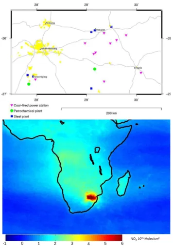
Results of tests of the iDOAS over the South African interior plateau, called the High-veld, are reported in this paper. The Highveld is the most highly industrialised region

10

in southern Africa (Fig.1), and satellite-detected NO₂column densities over the High-veld are the highest in the Southern Hemisphere and equivalent to those in the highly industrialised regions of east Asia, the Middle East, Europe and North America (Beirle

et al.,2006). Large power plants, synfuels refinery, metallurgical smelters, industries, mines and urban conglomerations on the Highveld are large area and point sources of

15

pollution. Stable atmospheric conditions in the region favour plumes to remain intact at large distances downwind of the sources. The Highveld is an ideal location to test the operation of a high resolution instrument like the airborne iDOAS

2 The measurement technique

The imaging DOAS technique was previously used in ground based applications ( Lo-20

hberger et al.,2004;Bobrowski et al.,2007) to map the trace gas distribution resulting from stack or volcano emissions. For that purpose the instrument was directed towards the interesting object (Fig.2). One section or column of the scene is imaged on the entrance slit of the spectrograph. The reflected and scattered sunlight is spectrally dispersed and recorded by a charge-coupled device (CCD). Each individual line of the

25

CCD chip corresponds to a spectrum and using the DOAS technique (Sect.2.3) results in one trace gas slant column density.

(5)

ACPD

Full Screen / Esc

Interactive Discussion The DOAS analysis yields a slant column density (SCD) which is the integrated

concentration along the light path (Sect. 2.3). In such a way, one section (column) of the respective trace gas distribution is observed. To obtain the two dimensional distribution of the slant column densities the instrument scans the scene perpendicular to the entrance slit (Fig. 2). In this study the results are mainly expressed as slant

5

column densities. They can be colour coded to illustrate the trace gas patterns. 2.1 Instrumental setup

The imaging DOAS instrument consists of an imaging spectrograph and a two dimen-sional detector i.e. a CCD camera. An optical system in front of the spectrograph focuses the incoming radiance onto the entrance slit. A large field of view (5−60◦_{) is}

10

mapped on the spectrograph. The height h of the entrance slit and the focal length f of the entrance optics determine the field of viewγ:

tan(γ/2) = h

2 · f (1)

The light entering the spectrograph is spectrally analysed and detected by the CCD. The DOAS analysis of the recorded spectra yields one column of trace gas information.

15

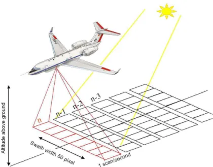
The instrument is installed on the aircraft with the entrance slit perpendicular to the flight direction. As the entrance optics generates a swath perpendicular to the flight direction, this technique is called push broom imaging. The principle is illustrated in Fig.3.

The aeroplane moves forward as a column of trace gas information is being recorded;

20

the resolution parallel to the flight direction is determined by the speed of the aircraft and the exposure time. After data from the CCD has been read out the next set of spec-tra is recorded. In the mean time the spec-trace gas contribution below the plane may have changed. In such a way, information about the two dimensional trace gas distributions below the aeroplane can be gained.

(6)

ACPD

Full Screen / Esc

Interactive Discussion The resolution perpendicular to the flight direction is determined by the

magnifica-tion of the optical system and the numbers of lines on the CCD chip i.e. 255 for our instrument. However due to the imperfect imaging qualities of the system (Sect.2.2) 8 lines have to be co-added, thus reducing the resolution to 32 lines perpendicular to the flight direction. Moreover the signal to noise ratio is improved, and the detection limit

5

reduced, when several CCD lines are co-added.

The instrumentation used for this study consists of an ACTON 300i imaging spectro-graph, which is a Czerny-Turner type with 300 mm focal length, an Andor DU-420BU CCD with 255 x 1024 pixel, and a mirror based entrance optics.

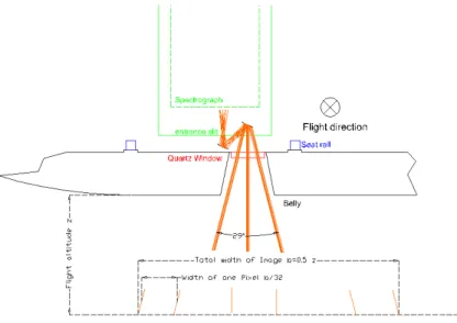
Details of the optical system are illustrated in Fig.4. The first mirror is convex with a

10

focal length of 51.5 mm and the second one is concave and has 25.6 mm focal length. The combination of both placed 70 mm apart results in the focal length of 13.7 mm. As the entrance slit is 6.9 mm high, according to Eq. (1) the total field of view is 28◦_{and the}

total field of view equals half the flight altitude above ground. As the sensitivity of the DOAS measurement strongly depends on the length of the light path through the trace

15

gas distribution, one might think that it would be more sensitive towards the edges of the images. However if the geometrical light path at the edges is compared to the nadir (centre), it is enhanced by 1/cos(14◦

)=1.03 i.e. only 3%.

In contrast to the ideal setup illustrated in Fig.4, the optical window in the aeroplane was a little bit too small, reducing the field of view to 24◦_{. Each swath was divided into}

20

27 ground pixels instead of 32. Assuming a standard flight altitude of 4500 m above ground level (a.g.l), the total swath was 1910 m wide and the lateral resolution was 71 m.

2.2 Characterisation of the instrument

To characterise the imaging quality of the instruments several tests with different light

25

sources were performed. Most artificial light sources had to be installed rather close to the instrument, hence the optical system tests was slightly different to the real mea-surements. One of the most convincing tests was to setup the instrument inside the

(7)

ACPD

Full Screen / Esc

Interactive Discussion hangar and direct it towards the doors. Each of the four doors was 4.5 m wide and the

distance to the instrument was 19 m. If the doors were opened by 30 cm, it resulted in three vertically extended light sources of 30 cm width separated by 4.5 m at a distance of 19 m from the instrument (Fig.5). The instrument’s total field of view is 9.5 m wide at the doors position.

5

A light source of 30 cm width at a distance of 19 m is expected to result in a spectrum of 255 pixels/9.5 m·0.3 m≈8 pixels on the CCD. The observed image is shown in Fig.6. The central spectrum has a full width of half maximum (FWHM) of 8 pixels. If the light source was made smaller (by closing the doors slightly) only a small decrease was observed, whereas if the doors were opened a clear increase in the width of the spectra

10

was visible. Therefore the minimum resolution of the complete system is approximately 8 pixels or 0.8◦

.

The minimum resolution along the flight direction is also determined by the optical system. If the motion of the plane is ignored or integration time is infinitely small, the instantaneous resolution would be 11 m at a flight altitude of 4500 m a.g.l. This has to

15

be added to the distance the plane travels during the actual integration time. In total the typical resolution ranges between 90 m and 200 m. A small gap (29 m) between the individual scans was caused by the CCD readout procedure, which lasted 0.4 s. The width of the gap also depends on the flight altitude; if the plane is flying low the gap is bigger, as the minimum resolution gets finer (Fig.10).

20

The iDOAS instrument was installed on the Rockwell Aerocommander 690A oper-ated by the South African Weather Service (ZS-JRA). The standard flight altitude was 6 km AMSL or 4.5 km a.g.l.; the speed ranged from 95 m/s to 135 m/s. The typical in-tegration time was about 1 seconds or less, hence the spatial resolution in the flight direction is about 100 m.

25

The exact instrument’s field of view relative to the aeroplane is very hard to de-termine, therefore the viewing direction is a bit uncertain, even if the exact roll and pitch angles were available. The total signal of the recorded light intensity divided by the integration time gives us a black and white image of the local surrounding

(8)

ACPD

Full Screen / Esc

Interactive Discussion which can be compared to more precise satellite images e.g. Google Earth images

http://earth.google.com. 2.3 DOAS Technique

To retrieve column densities from the observed spectra, the well known DOAS tech-nique (Platt,1994) is applied. The method is based on Lambert-Beer’s law.

5

The absorption cross section (σ) is a characteristic function of the wavelength λ

for the individual trace gases. The integrated concentration along the light path is called slant column density and is the result of the DOAS analysis. A normal in-flight spectrum in a remote and clean area is usually taken as the reference here. Thereby the Fraunhofer structures are removed from the fit and the stratospheric background

10

concentration is subtracted. However if the remote region is not as clear as expected, parts of the tropospheric signal are subtracted as well. Hence the results presented in Sect. 3 constitute lower limits of true tropospheric SCDs, they are usually referred to as differential slant column densities.

The wavelength range between 467 and 517 nm was chosen for the analysis and,

15

besides NO2, (Vandaele et al.,1997) the cross sections of water vapour (Rothman et

al.,1998), O₄(Hermans et al.,1999) and O₃(Burrows et al.,1999) were included. The filling in of the Fraunhofer lines due to inelastic Raman scattering (Ring effect) (Grainer

and Ring, 1962) was considered by using an appropriate cross section (Gomer et

al.,1996). The instrumental function varies across the CCD chip in both dimensions.

20

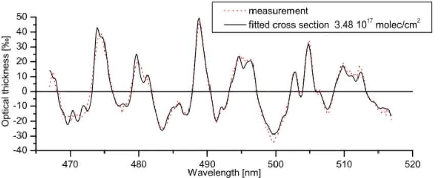
Therefore individual reference and ring spectra are applied in the fit for the spectra recorded in the respective regions of the CCD-chip. Moreover an individual calibration was used for each line. For the central CCD line a NO2 fit is shown in Fig. 7. The

spectrum was recorded on 5 October 2006 close to the synthetic oil refinery in Secunda (Fig.8and9).

25

The retrieved data is equivalent to the integrated concentration along the light path - the SCD. The tropospheric vertical column density (tVCD) is often a more accurate quantity for further analysis. It gives the integrated concentration across the altitude

(9)

ACPD

Full Screen / Esc

Interactive Discussion up to the mixing layer height and is therefore independent of the light path. The ratio

between slant and vertical column is called the air mass factor (AMF). It has to be simulated in a radiative transfer model. The complete light path between the instrument and the sun has to be considered for the model calculation. In this case the Monte Carlo-based radiative transfer model TRACY (Wagner et al.,2007;Deutschmann and 5

Wanger,2007) was used. The geometry of the setup including solar zenith angle was considered and the terrain altitude (1600 m) was included. The altitude is not quite correct for the entire Highveld, but within a range of 200 m no altitude dependency was observed in the simulation. Especially in dense plumes, aerosols can reduce the visibility; however, this effect was completely ignored here, as no significant change in

10

the O₄observation was detected. Due to emissions of water vapour clouds sometimes can be observed above power plants. This was not the case in the dry season on the Highveld. As the AMF calculation showed no strong variation between the different parts of the image, a constant AMF of 2.2 is used independent of the viewing direction. Most of the presented data are slant column densities. The flux estimate in Sect.3.3 15

is the only result where an AMF was applied.

3 Results

3.1 First measurement

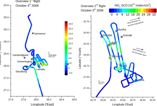
Three test flights over large pollution sources (coal-fired power plants, steel works and refineries) on the Highveld were flown on 4, 5 and 6 October 2006. The NO2 column

20

densities showed strong gradients in the immediate vicinity of various sources. An overview of the flight track from the first and the second flight (4 and 5 October 2006) is shown in Fig.8. The flight track and the observed NO2column densities of the third

flight are compared to SCIAMACHY data in Fig.14. Enhanced NO2column densities

are observed downwind of the plants. Here only the nadir direction (CCD-line 16) and

25

(10)

ACPD

Full Screen / Esc

Interactive Discussion During the 2nd flight the plume from Kendal power station was observed to merge

with the plumes from Matla and Kriel power stations to form one large plume which broadened with distance downwind. The plume of the synfuels refinery in Secunda was crossed three times at different distances downwind of the plant. The plume from the refinery is also observed to broaden and become more diffuse with distance from

5

the source.

3.2 Two dimensional NO₂distributions

Detailed 2-D images of the NO2 SCD close to selected sources are shown in Figs.9, 10and11.

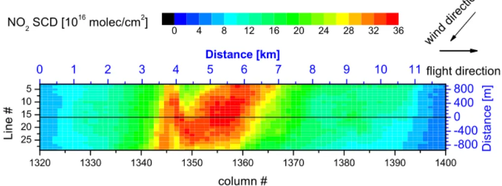
In Fig.9 the mixing of NO2 plumes originating from different sources in Secunda is

10

visible. Both plumes extend in different directions, which allows a qualitative altitude determination.

While the large plume seems to be close to the ground, according to the Eckmann spiral of wind direction the smaller one expands more perpendicular to the flight altitude and can therefore be expected to be at higher levels.

15

The spatial resolution at ground level theoretically increases when the flight altitude is lower. However, most of the point sources observed here do not emit the respective trace gases at ground level but at 250 m altitude. As the exit temperature of the emitted gases is usually quite high (on the order of 130◦

C for coal-fired power stations), effective stack height is several hundred metres above actual stack height, and there is a risk of

20

missing the plume or observing only parts of it when flying at lower altitudes.

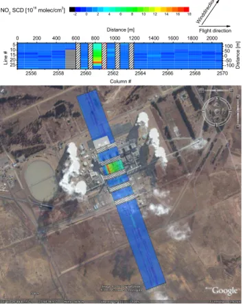
On 4 October 2007 the aircraft flew over Lethabo power plant in the Vereeniging area south of Johannesburg at 600 m a.g.l. (stack height 275 m; Fig. 10). The local enhancement in NO₂ column densities is observed in only a few pixels. Just north of the plant high intensity of reflected light (probably caused by the cooling tower or

25

the saturated plume above it) led to a blooming effect on the CCD, therefore no valid observation was made here. Although the plume was observed directly beneath the aeroplane and partly downwind, no widening of the plume perpendicular to the wind

(11)

ACPD

Full Screen / Esc

Interactive Discussion direction is observed. The plume broadens by less than one pixel (≈ 100m) at 150m

downwind of the stack, or it widens above the flight level and the effect cannot be observed by the downward looking imaging DOAS. Nevertheless the high resolution of 10 m perpendicular to the flight direction is still astonishingly good.

A typical plume expansion is observed close to the Majuba power plant (Fig.11top).

5

The image is overlaid in Fig.11(bottom) to a local satellite image (Google Earth). A strong enhancement in the NO2column is observed close to the stack. This is probably

caused by the long absorption path when looking on a rising plume from above. Further downwind the plume widens and the local column densities decrease as the plume turns from vertical to horizontal. The local enhancement at the downwind edge of the

10

image is not yet fully understood but seems to be a real change in the slant column density. It may be caused by the oxidation of NO to NO2 in the plume driven by the

mixing in of O3. Nitrogen oxides are mostly emitted as NO rather than NO2, typically

95% is NO. By reaction with O₃ it converts to NO₂ until the well known Leighton ratio establishes.

15

If the plume expands in vertical waves, this might again result in a locally extended absorption path through the plume. As the increase in the column density is higher than 3% the observation is not caused by the systematic difference in the sensitivity (Sect.2.1).

The position of the stack in Fig.11is determined based on the method described in

20

Sect.2.2.

3.3 Flux estimate

For the following flux estimate an AMF of 2.2 was applied to the SCD illustrated in Fig.11. To correct for a slightly enhanced background, the averaged column densities downwind of the power plant (first 8 lines of the image) were subtracted.

25

For selected distances downwind of Majuba the cross section of the vertical column densities are illustrated in Fig.12. The maximum of the column density is observed close to the stacks as mentioned above. The maximum flux (Fig. 13) however, is

(12)

ACPD

Full Screen / Esc

Interactive Discussion further downwind when the plume is wider.

After these preparations the flux was estimated by integrating the vertical column densities VCD along the local flight track (x-direction in Eq.2) considering the local wind speedvwindand wind directionα

flightdirection

wind relative to flight direction:

Φ = Z

VCD(x) · x · vwind· si n(α_windflightdirection) · dx (2)

5

The wind speed was not measured on board the plane but hourly averaged ground based observations are available in Majuba. The wind on this day 5 October 2006 was rather calm and blew with approximately 2.2 m/s from north western directions (≈ 296◦

) between 10:00 and 12:00 UTC. The observed NO2pattern (Fig.11) however,

indicates the wind direction was more from the north ≈ 330◦_{. The temporal variation in}

10

a 5 min interval can not be resolved by hourly averaged data, therefore during the mea-surements a northern wind direction does not contradict the measured wind direction in Majuba. Due to the high uncertainties in both methods the average wind direction (313◦_{) is considered in the flux estimates.}

Downwind of the source a linear increase in the total NO2flux is observed (Fig.13).

15

This of course does not necessarily indicate that additional sources are observed downwind, but it mainly results from the above mentioned NO oxidation and a parallel O3destruction.

Upwind of the source the flux is not zero. This might be caused by turbulent mixing near the buildings. It might also be caused by an insufficient background correction,

20

although the flux further away from the plume is far less. Instrumental effects should also not be neglected here. The exact direction in which the instrument is pointed cannot be determined; therefore the position of the enhanced NO₂columns relative to the real source might be shifted. As the resolution of the IDOAS instrument is quite good the observed increase cannot be explained by a sampling effect.

(13)

ACPD

Full Screen / Esc

Interactive Discussion 3.4 Comparison with SCIAMACHY

A first comparison of the iDOAS measurements with SCIAMACHY tropospheric slant columns is shown for the flight on 7 October 2006 in Fig. 14. The finer resolution iDOAS data can be averaged perpendicular to the flight direction for comparison with the satellite instrument.

5

South of Johannesburg in the industrial region around Vereeniging high column den-sities were observed. The enhanced local concentrations also lead to an increase in the SCIAMACHY NO2 data. The large field of view of SCIAMACHY however, is

domi-nated by the low column densities outside the industrial areas. Hence we can estimate the NO2variability inside one SCIAMACHY pixel to be rather high, as the enhancement

10

seems to be caused by high column densities in a small area, whereas the surrounding areas seems to be much cleaner.

For the detailed interpretation the temporal mismatch has to be considered. The aeroplane arrived at Sasolburg at 09:55 and returned at 11:25 UTC. ENVISAT (SCIA-MACHY) crossed the same area 2 h previously at 07:46 UT. Within these 2 morning

15

hours the atmospheric conditions might have changed significantly.

4 Conclusions

We presented the first direct observations of two dimensional NO₂ distributions over the industrialised Highveld in South Africa. Based on the observed NO2patterns two

different sources in close proximity to one another can be distinguished, and qualitative

20

altitude determination can be made.

NO2 flux estimates are possible on the basis of vertical columns and the wind data.

Athough the maximum column density partly decreases with distant to the stack, an overall increase in the NO₂ flux is observed. Both the widening of the plume and the NO to NO₂conversion attribute to this effect. A radiative transfer model was used for

25

(14)

ACPD

Full Screen / Esc

Interactive Discussion plume have not yet been considered. These data could also be compared to data

provided by the plant operators.

Slant column densities were compared to satellite data (SCIAMACHY). Although the different spatial resolution of satellite instruments results in large discrepancies be-tween finer resolution iDOAS measurements and coarser resolution satellite

measure-5

ments (Heue et al.,2005), detailed knowledge about the local distribution inside the satellite pixels is of great interest. For a more quantitative comparison special flights have to be performed, during which the flight is coordinated with satellite overpass time.

To improve the pointing accuracy of the iDOAS, a digital camera will be installed next

10

to the spectrometer. This will give additional information on the area over which the flight is conducted.

The actual wavelength range of the instrument is optimised for NO2, but several

in-teresting trace gases e.g. SO₂ and HCHO show strong absorption bands in the UV (300–400 nm). Future measurement flights will use a slightly different instrument

opti-15

mised for the observation of these trace gases as well.

Additional measurement flights in the Highveld (South Africa) were performed in August 2007 and March 2008, in order to validate the satellite retrievals on a regional scale and investigate individual sources on a local scale. The analysis of this data is still in progress.

20

Acknowledgements. Financial support for this research project was provided by Eskom Cor-porate Services as part of their Research and Development Programme and is gratefully given credits. Thanks to the South African Weather Service for the support of the aeroplane and the logistical support in Bethlehem, including the daily weather briefing.

References 25

Bobrowski, N., Glasow, R.v., Aiuppa, A., Inguaggiato, S., Louban, I., Ibrahim, O. W., and Platt, U.: Reactive Halogen Chemistry in Volcanic Plumes, J. Geophys. Res., 112, D06311,

(15)

ACPD

Full Screen / Esc

doi:10.1029/2006JD007206, 2007. 11881

Beirle, S., Platt, U., von Glasow, R., Wenig, M., and Wagner, T.: Estimate of nitrogen ox-ide emission from shipping by satellite remote sensing, Geophys. Res. Lett., 31, L18102,

doi:10.1029/2004GL020312, 2004. 11881

Beirle, S., Platt, U., and Wagner, T.: Potential of monitoring nitrogen oxides with satel-5

lite instruments, Procceeding of The 2006 EUMETSAT Meteorological Satellite Confer-ence, Helsinki, Finland, http://www.eumetsat.int/Home/Main/Publications/Conference and

Workshop Proceedings/groups/cps/documents/document/pdf conf p48 s4 02 beirle v.pdf 12–16 June 2006, last access: 3 June 2008. 11881,11894,11907

Burrows, J. P., Richter, A., Dehn, A., Deters, B., Himmelmann, S., Voigt, S., and Orphal, J.: 10

Atmospheric remote-sensing reference data from GOME: Part 2. Temperature-dependent absorption cross-sections of O₃ in the 231–794 nm range, J. Quant. Spectrosc. Ra., 61,

509–517, 1999. 11885

Deutschmann, T. and Wagner, T.: Tracy User manual, Universit ¨at Heidelberg, 2007.11886

Grainger, J. and Ring, J.: Anomalous Fraunhofer line profiles, Nature, 193, 762, 1962.11885

15

Gomer, T., Brauers, T., Heintz, F., Stutz, J., and Platt, U.: MFC 1.98 m User Manual. Institut f ¨ur

Umweltphysik, 1996. 11885

Hartl, A., Song, B. C., and Pundt, I.: 2-D reconstruction of atmospheric concentration peaks from horizontal long path DOAS tomographic measurements: parametrisation and geometry within a discrete approach, Atmos. Chem. Phys., 6, 847–861, 2006,

20

http://www.atmos-chem-phys.net/6/847/2006/. 11880

Heue, K.-P., Richter, A., Bruns, M., Burrows, J. P., Friedeburg, C. v., Platt, U., Pundt, I., Wang, P. and Wagner, T., Validation of SCIAMACHY tropospheric NO2-columns with AMAXDOAS measurements, Atmos. Chem. Phys., 5, 1039–1051, 2005,

http://www.atmos-chem-phys.net/5/1039/2005/. 11891

25

Heue, K.-P., Wagner, T., Broccardo, S. P., Piketh, S. J., Ross, K. E., and Platt, U.: Direct Obser-vation of two dimensional trace gas distribution with an airborne Imaging DOAS instrument, Proceedings of the ESA Conference on Rockets and Balloons and related research, 4th–7th

June 2007, Visby, Sweden, 2007. 11902

Hermans, C., Vandaele, A. C., Carleer, M., Fally, S., Colin, R., Jenouvrier, A., Coquart, B. and 30

Mrienne, M. F.: Absorption-cross sections of atmospheric constituents: NO₂, O₂ and H₂O, Environ. Sci. Pollut. Res., 6, 3, 151–158, 1999.11885

(16)

absorp-ACPD

Full Screen / Esc

tion spectroscopy of atmospheric gases, Appl. Optics, 43, 24, 4711–4717, 2004. 11881,

11895

Rothman, L. S.: The HITRAN molecular spectroscopic database and HAWKS (HITRAN Atmo-spheric Workstation): 1996 edition, J. Quant. Spectrosc. Ra., 60, 5, 665–710, 1998. 11885

Platt, U.: Differential Optical Absorbtion Spectroscopy (DOAS), in: Monitorting by spectroscopic 5

techniques, edited by: Sigrist, M. W., New York: John Wiley & Sons, Inc, 1994.11885

Vandaele, A. C., Hermans, C., Simon, P. C., Carleer, M., Colin, R., Fally, S., Mrienne, M.-F., Jenouvrier, A., and Coquart, B.: Measurements of the NO2 Absorption Cross-section from 42 000 cm−1 _{to 10 000 cm}−1 _{(238–1000 nm) at 220 K and 294 K, J. Quant. Spectrosc. Ra.,}

59, 171–184, 1997.11885

10

Wagner, T., Burrows, J. P., Deutschmann, T., Dix, B., von Friedeburg, C., Frieß, U., Hendrick, F., Heue, K.-P., Irie, H., Iwabuchi, H., Kanaya, Y. Keller, J., McLinden, C. A., Oetjen, H., Palazzi, E., Petritoli, A., Platt, U., Postylyakov, O., Pukite, J., Richter, A., van Roozendael, M., Rozanov, A., Rozanov, V., Sinreich, R., Sanghavi, S., and Wittrock, F.: Comparison of box-air-mass-factors and radiances for Multiple-Axis Differential Optical Absorption Spectroscopy 15

(MAX-DOAS) geometries calculated from different UV/visible radiative transfer models,

At-mos. Chem. Phys., 7, 1809–1833, 2007, http://www.atmos-chem-phys.net/7/1809/2007/.

(17)

ACPD

Full Screen / Esc

NO21015Molec/cm2

0 1 2 3 4 5

-1 6

Fig. 1. Map of the Heighveld including the position of the main industries. Averaged

(18)

ACPD

Full Screen / Esc

(19)

ACPD

Full Screen / Esc

(20)

ACPD

Full Screen / Esc

Fig. 4. Details of the mirror based entrance optics looking from the back of the aircraft. The

total swath width equals half the flight altitude and is divided into 32 pixels. Due to obstruction from the belly only 27 pixels receive a significant signal.

(21)

ACPD

Full Screen / Esc

Fig. 5. Ground setup used to characterise the optical properties of the airborne iDOAS. Each

hangar door was 4.5 m wide and the small openings in between were 30 cm, hence the total distance between the light sources was 9.9 m (edge to edge).

(22)

ACPD

Full Screen / Esc

Fig. 6. CCD image of the three hangar doors. Only parts of the outermost slits are observed.

This is expected as the distance between the doors and the instrument is less than double the distance between light sources. The total chip is 255 lines wide and the illuminated area in the centre covers 8 lines.

(23)

ACPD

Full Screen / Esc

Printer-friendly Version Interactive Discussion 470 480 490 500 510 520 -40 -30 -20 -10 0 10 20 30 40 50 O p ti ca l th ickn e ss [‰] Wavelength [nm] measurement

fitted cross section 3.48 1017

molec/cm2

Fig. 7. Example fit of the DOAS Analysis for NO₂. The analyzed spectrum was observed on 5 October 2006 downwind of Secunda synfuel refinery (spectrum 1355 line 16).

(24)

ACPD

Full Screen / Esc

Printer-friendly Version Interactive Discussion 27.6 27.8 28.0 28.2 28.4 28.6 -27.2 -27.0 -26.8 -26.6 -26.4 -26.2 -26.0 -25.8 Vanderbijlpark Vereeninging Sasolburg L a ti tu d e [° S o u th ] Longitude [°East] -2.0 0 2.0 4.0 6.0 8.0 10.0 12.0 14.0 16.0 18.0 Overview 1st flight October 4th 2006 Lethabo Samancor 10 km 28.75 29.00 29.25 29.50 29.75 30.00 30.25 -27.25 -27.00 -26.75 -26.50 -26.25 -26.00 -25.75 Duvha Kendal Komati Kriel Majuba Matla Tutuka Secunda Wind dire ction in

the free tropo

sphere Lati utde [° S outh] Longitude [°East] Wind d_irection in the bou ndary layer NO₂ SCD [1016 molec/cm2 ] 10 km Overview 2nd flight October 5th 2006 0 4 8 12 16 20 24 28 32

Fig. 8. Overview of the tracks of the flight on 4 and 5 October 2006 close to pollution sources.

(25)

ACPD

Full Screen / Esc

Printer-friendly Version Interactive Discussion 0 1 2 3 4 5 6 7 8 9 10 11 -800 -400 0 400 800 5 10 15 20 25 1320 1330 1340 1350 1360 1370 1380 1390 1400 column # L in e # 0 4 8 12 16 20 24 28 32 36 NO₂ SCD [1016 molec/cm2] flight direction win d di rect ion D is ta n c e [ m ] Distance [km]

Fig. 9. NO₂ SCD close to the synthetic fuel refinery in Secunda, showing the mixing of two plumes (Heue et al.,2007). Both plumes probably originate from the refinery but from different sources, however they can clearly be resolved. The gaps (Fig.10) between the individual columns are not shown as they are rather small due to the flight altitude

(26)

ACPD

Full Screen / Esc

Printer-friendly Version Interactive Discussion 0 200 400 600 800 1000 1200 1400 1600 1800 2000 -100 -50 0 50 100 5 10 15 20 25 2556 2558 2560 2562 2564 2566 2568 2570 Column # L in e # -2 0 2 4 6 8 10 12 14 16 18 NO₂ SCD [1016 molec/cm2 ] Distance [m] D is ta n c e [ m ] Flight direction Win ddire ctio n

Fig. 10. Enhanced NO₂SCDs over the stack of Lethabo power station 4 October 2006. The CCD was partly oversaturated leading to a blooming effect; hence no data are shown just north of the plant. No spectra are observed during the read out process indicated by the hashed areas. This also holds for the rest of the observation but is only shown close to the power plant. Compared to Fig.9and Fig. 11the flight altitude is significantly lower, therefore the pixels are smaller here. An overlay to a Google Earth map is shown in the lower panel.

(27)

ACPD

Full Screen / Esc

Printer-friendly Version Interactive Discussion 0 500 1000 1500 2000 2500 3000 3500 4000 4500 5000 5500 6000 -800 -600 -400 -200 0 200 400 600 800 5 10 15 20 25 4380 4385 4390 4395 4400 4405 4410 4415 4420 Column # lin e # 0 2 4 6 8 10 12 14 16 18 20 22 24 NO₂ SCD [1016 molec/cm2 ] flight direction w in_d d ire_c tio_n D is ta n c e [ m ] Distance [m]

Fig. 11. NO₂SCD (top) around the Majuba power plant (5 October 2006) overlay over a local map (bottom). Same flight level as Fig.9, hence the pixels are wide again and the gaps are not shown. The arrows in the top figure indicate the position of the respective cross sections shown in Fig.12. The circle shows the approximate position of the plant.

(28)

ACPD

Full Screen / Esc

Printer-friendly Version Interactive Discussion 1000 2000 3000 4000 5000 -1 0 1 2 3 4 5 6 7 8 9 10 V e rt ic a l c o lu m n d e n si ty [1 0 1 6 m o le c/ cm 2 ]

Distance (x) along the flight [m]

CCD8 CCD14 CCD18 CCD23 CCD28

Fig. 12. Cross sections through the plume along the flight direction. The respective line are

(29)

ACPD

Full Screen / Esc

Printer-friendly Version Interactive Discussion -200 0 200 400 600 800 1000 0.0 0.5 1.0 1.5 2.0 # 14 # 18 # 23 F lu x [ 1 0 2 4 m o le c /s ]

Approximated distance down wind of the stacks [m] NO

2 Flux

Linear Fit # 28

Fig. 13. NO₂flux downwind of the Majuba power plant. Upwind of the stack the NO₂columns are slightly enhanced. Perhaps the positions of the stacks are not known precisely enough or the low wind speeds allows some turbulent mixing close to the buildings.

(30)

ACPD

Full Screen / Esc

Fig. 14. Comparison between SCIAMACHY tropospheric SCD (Beirle et al., 2006) and the averaged iDOAS column density data from 6 October 2006. Strongly enhanced column densi-ties were observed by the Imaging DOAS instrument in the industrial area around Vereeniging. Due to the large sampling area of SCIAMACHY the local enhancement affect the satellite ob-servations only slightly.