Cheap talk and costly consequences

Cheap Talk and Costly Consequences

by

Isabella Loaiza Saa

Submitted to the Program in Media Arts and Sciences,

at the School of Architecture and Planning,

in partial fulfillment of the requirements for the degree of

Master of Science in Media Arts and Sciences

at the

MASSACHUSETTS INSTITUTE OF TECHNOLOGY

September 2019

@Massachusetts

Institute of Technology 2019. All rights reserved.

Author

...

Signatureredacted

Program in Media Arts and Sciences,

at the School of Architecture and Planning,

August 18, 2019

Signature redacted

C ertified by ...

V' ~ex('Sandy') Pentland

Toshiba Professor of Media Arts and Sciences

Thesis Supervisor

Signatureredacted

Accepted by ...

MASSACHUSETTS INSTITUTE

Tod

achover

OFTECHNOLOGY

Academic H

d, Program in Media Arts and Sciences

OCT

0 4

2019

Cheap Talk and Costly Consequences

by

Isabella Loaiza Saa

Submitted to the Program in Media Arts and Sciences, at the School of Architecture and Planning, on August 18, 2019, in partial fulfillment of the

requirements for the degree of

Master of Science in Media Arts and Sciences

Abstract

In this thesis, we use data on political interactions between country pairs to predict changes in trade. We implemented and applied a new feature selection algorithm called Boruta to build a compact set of predictor variables for this task. After finding a consistent set of features we used a Random Forest Classifier to predict bilateral changes in trade between 1998-2014. To better understand the contribution of each of the predictor variables used in the model we employ three different methods for calculating feature importance. Our results suggest that political and diplomatic interaction at at least as important (if not more) as distance and for predicting changes in trade.

Thesis Supervisor: Alex ('Sandy') Pentland

Cheap Talk Costly Consequences

by

Isabella Loaiza Saa

This dissertation/thesis has been reviewed and approved by the following committee members

Signature redacted

Thesis advisor ...

Alex ('Sandy') Pentland Toshiba Professor of Media Arts and Sciences Program in Media Arts and Sciences

Signature redacted

T hesis reader...

EstanMoro Associate Professor Universidad Carlos III de Madrid

Thesis reader

...

Signature redacted

....

Moshe Hoffman Research Scientist

Acknowledgments

I would like to thank my thesis advisor Alex Pentland for his guidance and patience in this journey. I would also like to thank my thesis readers for their time and help.

I am thankful for my friends and colleagues Areen, Abdulrahman, Andres, Carlos

R., Cesar U., Dhaval, Eduardo C., Jonas, Judy, Leo, Morgan, Nelson G., Pedro C., Sam H., Samantha G., Sandro, Tara, and Zivvy, who have helped and supported me through difficult times. Thanks to the members of the MIT Colombian Association and our friends at the Harvard Student Society of Colombia for making Boston feel a bit more like home.

Finally, I'd like to thank my family for their encouragement, love and understand-ing.

Contents

1 Introduction . . . . 15 2 Related W ork . . . . 17 2.1 Liberal Peace . . . . 17 2.2 Economic Diplomacy . . . . 18 3 Data . . . . 19 4 M ethods . . . . 23 4.1 Feature Selection . . . . 23 4.2 Prediction . . . . 26 4.3 Accuracy Benchmarks . . . . 26 4.4 Feature Importance . . . . 28 5 Results . . . . 30

5.1 Prediction Accuracy Benchmarks . . . . 30

5.2 Feature Significance . . . . 31

5.3 Feature Importance . . . . 33

6 Limitations . . . . 37

List of Figures

1 Distributions of predictor features. . . . . 21

2 Distributions of predictor features and target variable . . . . 22

3 Model Accuracy by Year. . . . . 30

4 Average Accuracy for training set . . . . 31

5 Average Accuracy for test set. . . . . 31

6 Feature Importance Boxplot. . . . . 34

7 Feature Importance Boxplot 2 . . . . 35

8 Permutation Importances using accuracy score as target metric. . . 35

9 Dropping Column Importances with F1 score as target metric. .... 36 10 Dropping Column Importances with Accuracy score as target metric. 36

List of Tables

1 ParameterSetsforGridSearch. . . . . 26

1

Introduction

The relationship between international trade flows and the political and social in-teractions between countries has interested political scientists and economists alike. This relationship has mostly been studied in one direction: How does trade affect international conflict or cooperation. Considered as one of the elements of 'liberal peace' or 'Kantian peace' inquiries into the impact of trade on international relations has had a long tradition dating back to the 1 8th Century. Thinkers like Montesquieu and Kant already posed the idea that trade fostered peaceful interactions between nations. A closer examination of the relationship between trade and conflict in the opposite direction, however, is still required.

Interest in unpacking the effects of political relations on international trade has recently been revived thanks to the recent financial crisis, the increase in economic interdependence, and the growing relevance of centrally planned economies in inter-national markets [26]. The current conditions, thus, give way to the re-emergence of the field of economic diplomacy. Economic diplomacy can roughly and briefly be understood as 'the management of relations between states that affect international economic issues intending to foster prosperity.' Research in this area has sought to quantify the effects of diplomatic and political interactions in international trade using the infrastructure of embassies and consulates

1341,

official diplomatic visits between governments

13],

UN voting behavior

114],

and political interactions. Most of the work fits into categories 1 and 2, in part because of how these can be interpreted as signal-ing the health of the diplomatic relation between the countries involved. However, we still need to better understanding how more transitory, 'less costly', non militarized interactions affect trade between countries.

Studying the political interactions under the third category is especially relevant in a world where the digital revolution has made some scholars and practitioners question the utility and functions of a network of diplomatic posts

121].

Further, because digital news sources reporting on political and diplomatic events can be accessed almost anywhere, digital media has become an unquestionable channel for

diplomatic communication and has reshaped the practice of diplomacy globally 12, 9]. As technology has brought fundamental changes to diplomacy, it has too changed economic diplomacy [2].

This work seeks to quantify the effect of political interactions in international trade flows on a global scale. In particular, it sheds some light on the questions: What is the effect of foreign political relations in changes in bilateral trade? How does the predictive power of verbal political interactions differ from the predictive power of the whole set of political interactions when forecasting changes in trade?

In addition to studying how political interactions alter changes in trade in the context of the information age, this work is relevant because it uses a large-scale data set that encompasses many countries across the globe. According to [40], studies in economic diplomacy have provided limited evidence since most of the data sets used for research only include a selected group of countries, rendering their evidence more limited. Some authors report similar shortcomings in a meta-analysis of 32 papers relating to economic diplomacy [291. We contribute by expanding these studies by including over 50 number of countries in our analysis, 1399 country pairs or dyads over 16 years. Our data set is also more recent; much research on this question has been carried out using older data sets, for example

[301

used data from 1885 to 1992. These data sets pre-date essential events that have shaped the current state of global security and international trade like September 11 and the 2008 credit crunch.

The current work is organized as follows: First, we briefly summarize related work. Second, we explain the data used together with the methods. We continue with a description of our results, and a section about the limitations of this work. We finalize with a discussion and suggestions about future work.

2

Related Work

2.1

Liberal Peace

The power of trade as a deterrent of war is among the most fundamental ideas in political science and economics. As early as the 1 8t' Century, de Montesquieu

1151

claimed that trade forged a peaceful union between nations driven by mutual neces-sities. Two hundred years later, this idea helped promote the consolidation of the European Union [16]. Today, the World Trade Organization (WTO) lists supporting peace and stability as one of the benefits of trade between nations [1]. In spite of three hundred years of coming into the mainstream of classical economic thought, the idea that trade promotes peace has recently been put up for debate

1181.

Some studies found that trade 'follows the flag' suggesting that political interests precede trade and therefore its effect as a deterrent of war are insignificant [24, 39]. Other work presents a milder counter-argument claiming that this idea is only partially correct [251. As more research in response to these discrepancies continues to provide evidence of the pacifying effects of trade interdependence [20, 221, there seems to be room for further contributions to this topic.

The roots of the myriad of mechanisms proposed as drivers of the hampering effect of trade on war range from fundamental economic theory to community-based arguments to social learning. Mechanisms stemming from economics include strict or relative [31, 33]dependency, access to goods

[41

raised opportunity costs of war [37], and gains from the growth of domestic economies through international commerce

[35] are among the first and most widely studied mechanisms. The second set of

mechanisms found in the literature are community-based mechanisms that explain the pacifying effects of trade from the sentiment of belonging to a global community. The following group of mechanisms has recently received attention thanks to the rise of network analysis methodologies, which allowed the study of direct and indirect effects trading ties and trading blocs [28]. In contrast, social learning mechanisms such as the flow of information, the alignment of national incentives, and the creation of mutual understanding, while introduced during the latter part of the 1 9thCentury

have not been studied empirically but are frequently mentioned in the literature

[171.

2.2

Economic Diplomacy

As previously mentioned, the term economic diplomacy has been used in recent years to refer to the use of political or diplomatic tools to achieve economic goals by reducing intangible trade barriers like government frictions or institutional differences.

Economic diplomacy might have traditionally concerned the foreign policy agenda, but with globalization, the line between the domestic and foreign is increasingly blurred. Similarly, the digital age has increased the velocity with which political events are communicated, and it has reinforced the role of non-state actors such as NGOs, activists, and firms in political and diplomatic discussions regarding the

economy [21, 7].

While the link between politics and trade might not be readily apparent [40] describe three different ways in which the government might get involved in trade:

1. The type of product might require the involvement of the government. An

example of this instance is the purchase of military equipment.

2. Intervention via state/public enterprises. Here, recent evidence supports the hypothesis that trade with state-owned companies is more sensitive to political relations than trade originating from private companies

114].

3. Signaling from high ranking political actors about the desirability (or not) to

develop commercial relationships with other nations.

The research in economic diplomacy using diplomatic posts has found even dice of positive effects of economic diplomacy in trade [23, 34]. However, such results need to be extended for the types of interactions we seek to study in the present work.

3

Data

To study the effects of political interactions in trade, we combine data sets about political interactions, international trade, distance, and country GDPS.

To measure political interactions, we use the open-source ICEWS dataset [10]. ICEWS is a large-scale, event-driven data set that aggregates daily interactions be-tween many actors in over 100 countries. Mined from diverse news sources around the world, it encodes over 300 types of events and classifies them according to the Conflict and Mediation Event Observations taxonomy (CAMEO). This classification helps map interactions to a Goldstein Score

[191,

which describes the event's level of cooperation or hostility. Goldstein Scores range between -10 and 10, where nega-tive scores signal conflict and posinega-tive ones signal cooperanega-tive actions. By taking the average Goldstein Score per year, we built directed time series of political relations between 1399 country-pairs between 1998-2013.

Particularly interesting to the work proposed here is the ability to cross-reference the kinds of actions taken by aggregated generic actors (e.g., police, government, activist, business) within nations. As digital technologies have increased the par-ticipation of non-state actors in political affairs, we use all interactions in the data set regardless of the source actor. Including all interactions and not just those com-ing from government officials allows us to capture diplomatic interactions in a more realistic way as opposed to a void where only government actors interact.

The data on international trade comes from, the Observatory of Economic Com-plexity {5]. This data contains trade flows disaggregated by origin and destination from 1962 to 2014. For our predictive model, we use exports, as opposed to total trade. Using exports reflects the directed aspect of the political interaction time-series. Thus, we aggregate exports by year regardless of product type and create time series for all of our country pairs. Future work could aim at taking advantage of the trade classifications in this data - HS and SITC - and quantifying the effect of political relations to different types of products or commodities.

on distance between country is measured as the distance between country capitals. Our unit of analysis for this research is the yearly country pair, comprised by the source country the target country. To clean and merge the data for prediction, we decided to drop pairs that have less than four, consecutive yearly interactions, because we considered that would be a very sparse political relationship. We also removed country pairs for which we did not have data on the GDP of one or both countries. Since the ICEWS data is directed, we don't use total trade, but instead, we use only exports, rendering pair (A, B) different from pair (B,A).

To prepare our target variable for our prediction task, we correct the total exports from Country A to Country B by dividing it into the product of the countries' GDPs for that year. Then, we take the percent change between that year yt and the previous year yt-1. The purpose of doing this is two-fold: First, this helps us intuitively binarize our target variable, and it also makes it stationary.

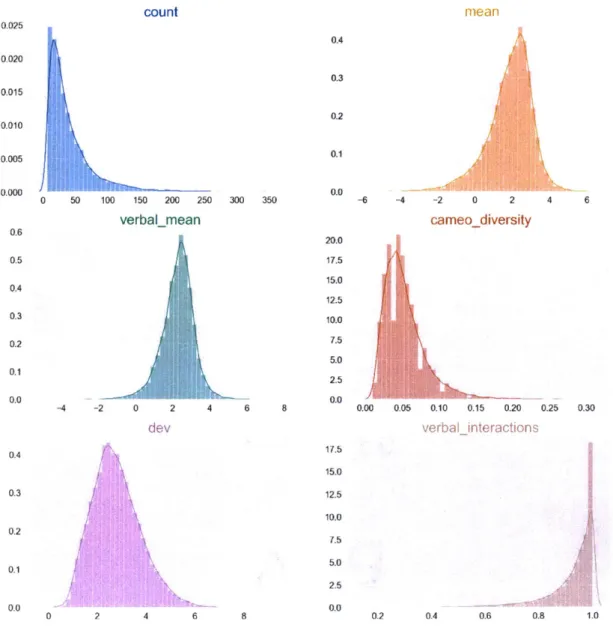
After cleaning our data, we check if the variable distributions are well behaved. The distributions are depicted in Figures 1 and 2.

count I 0.000 0 50 100 150 200 250 300 350 verbalmean 0.6 0.5 0.4 0.3 0.2 0.1 -4 -2 0 2 4 6 dev 0 2 6 8 8 0.4 0.3 0.2 0.1 0.0 20.0 17.5 15.0 12.5 10.0 7.5 5.0 2.5 0.0 17.5 15.0 12.5 10.0 7.5 5.0 2.5 0.0 mean 11 -6 -4 -2 0 2 cameodiversity

a4

4 6 0.00 0.05 0.10 0.15 0.20 0.25 0.30 verbalinteractions 0.2 0.4 0.6 0.8 1.0

Figure 1: Distributions of predictor features.

This figure shows the distribution plots of the predictor features used in the classifier. All were computed using ICEWS data and capture some aspect of the political interactions

between country pairs.

0.025 0.020 0.015 0.010 0.005 0.0 0.4 0.3 0.2 0.1 0.0

gdpasym -10 -5 0 5 10 exports-lagged M 1.5 1.0 0.5 0.0 - """ -0.75 -0.50 -0.25 0.00 0.25 0.50 0.75 changegdp-b 3.5 3.0 2.5 2.0 1.5 1.0 ,. export 1.0 0.8 0.6 0.4 0.2 0.0 0.0 0.5 1.0 1.5 2.0 2.5 3.0 3.5 4.0 changegdp_a 3.5 3.0 2.5 2.0 1.5 1.0 0.5 0.07 - -.--0.75 -0.50 -0.25 0.00 0.25 0.50 0.75 1.00 1.25 0.5 -0.75 -0.50 -0.25 0.00 0.25 0.50 0.75 1.00 1.25 "

Figure 2: Distributions of predictor features and target variable

This figure shows the distribution plots of the predictor features and the target variable

exports lagged used in the classifier. GDP data was take from the World Bank.

22 0.14 0.12 0.10 0.08 0.06 0.04 0.02 0.00

4

Methods

Our goal is to understand the effects of political interactions on international trade and predict the changes in trade levels between countries in our data using information about their political relations. By predicting changes in trade instead of the quantity or value of goods that are traded, the prediction task becomes a more straightforward, binary classification task. Hence, we use a Random Forest classifier

[11]

that we train on features about political interactions extracted from ICEWS as well as other macro-economic related features.

As it is usual for prediction tasks where the set of features that could be used is reasonably large, we first build a set of plausible features and perform feature selection to keep the ones with the highest predictive power. Since our goal is not just to build a black-box model, but gain insights into the relationship between our predictor variables and target, we create a compact set of twelve features using our expert knowledge and previous findings on the field of international relations. From this initial set, we only keep the features deemed significant by our feature selection algorithm and use those in our model. Keeping in mind the impact of choice of features over the choice of the model on performance led us to spend considerable effort on feature selection and feature engineering. In line with our research goals, we chose an all-relevant feature selection algorithm over a minimal set feature selector.

4.1

Feature Selection

Feature selection was an essential part of the present work, especially for the multitude of explanatory variables that could dictate changes in international trade. Keeping in mind that model interpretability and understanding the dynamics between politics and international trade is the goal here, an all-relevant feature section algorithm is best suited for our needs. All-relevant algorithms are better for understanding the relationship between the features and the target because they can detect all the features relevant for the phenomenon at hand, instead of only the non-redundant ones, even the features that are only relevant when used in conjunction with others.

We use the Boruta algorithm [27] that has quickly become a popular choice for this kind of feature selection. It is built around random forest classifiers or regressors, making it robust to overfitting and its level of false positives is low, with on average less than one falsely relevant variable detected in the different tests by 1361.

As opposed to methods that find the minimal set of features to optimize prediction accuracy, Boruta assumes that while the degradation of the classification accuracy after the removal of the feature from the predictor set, is enough to deem the feature important, the lack of this effect is not sufficient to deem it unimportant.

Boruta consists of the following steps:

1. Creation of at least five shadow features: New shadow features are added

to the data set by permuting the original features. By permuting the observa-tions in the shadow, features should be as good at predicting the target variable as random noise while maintaining some properties of the original features like its distribution.

2. Find feature importance: The importance of all features in the extended

data set is measured by obtaining their Z-scores after running a Random Forest classifier.

3. Recording hits: Find the maximum Z-score among the shadow features, or

MZSA. For each original feature, check whether or not its Z-score is larger than the MZSA. If so, record this as a hit.

4. Detecting statistically significant features: Steps 1-3 are repeated for n iterations. The importance measure itself varies due to the stochasticity of the Random Forest Classifier. Therefore, we need to repeat the re-shuffling procedure to obtain statistically valid results. After the nth iteration, all original features have a list recording the number hits.Any original feature can have at most n hits, which means that it outperformed the best shadow feature in all n iterations. Most often,a given feature is going to have a number of hits between zero and n. To test if each feature is performing statistically better than the

best shadow feature, Boruta employs a bimodal test. If the null hypothesis is rejected, the feature is classified as significant. If the null hypothesis is accepted, the feature is classified as insignificant.

In summary, Boruta creates shadow features as a benchmark to compare features, thus measuring their relative importance. However, instead of comparing the original features to random noise, by creating noisy features out of the original ones, the shadow features keep specific characteristics that are unobserved to the researcher. Since the shadow feature retains these properties, the probability that original feature outperforms its respective shadow feature by the solely because of this characteristic is very low.

Boruta also includes some corrections for testing the significance of a feature against the shadow feature, since a simple hypothesis test cannot be performed due to the following reasons:

1. Features are not tested against a single alternative; instead, they are tested

against the maximum score among all shadow features. If there are many

shadow features, it might be likely that one of the shadow features is extraor-dinarily large. Thus, an important feature might be falsely rejected. The algo-rithm accounts for this by applying a Benjamini Hochberg False Discovery Rate correction term, to guard against what is known as Type I Errors in statistics. 2. At iteration n, the tests have been performed n - 1 times. If n is large enough,

a non-important feature can be detected as important by the sheer number of tests that have been performed. The algorithm corrects for this by using a Bonferroni correction term.

Due to the 'relative importance' fashion of determining significant features, Boruta could potentially deem a feature as significant even though it should not be. To gather a more consistent set of significant features, we explore a rather small set of parameters settings and only keep features that have been classified as significant for more than 60% of the parameter settings. To prevent data leakage caused by using the entire dataset for feature selection, we only use Boruta on the training data set.

4.2

Prediction

We applied a Random Forest classifier to predict the sign of change in trade between country pairs. We chose to use a Random Forest Classifier because they are widely used, relatively robust to overfitting, easily parallelizable, and provide variable impor-tance measures. While it has been shown that Random Forests don't fit time-series data well because of their inability to detect increasing or decreasing trends found in many time-series, this isn't a concern in our model. Our target time series is station-ary because the target variable is changes in trade, not the volume of trade between country pairs.

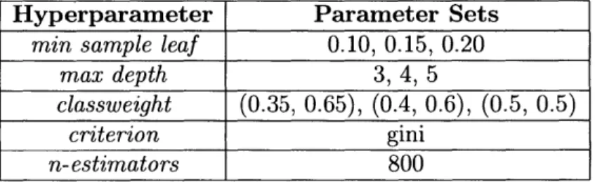
To tune the model hyperparameters, we use scikit learn' s grid search with a relatively small set of parameters to explore. In conjunction with GridSearch, we also use 10-fold cross-validation to avoid overfitting. The best model kept for prediction is the one that scored higher using the area under the curve as the metric of choice. Table 1 shows the parameters that were used with GridSearch to determine the best model for our task.

Hyperparameter Parameter Sets

min sample leaf 0.10, 0.15, 0.20

max depth 3,4,5

classweight (0.35, 0.65), (0.4, 0.6), (0.5, 0.5)

criterion gini

n-estimators 800

Table 1: Parameter Sets for GridSearch.

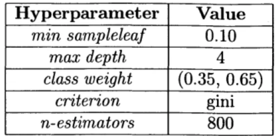
The best model hyperparameters used in the final model are shown in Table 2. Since the target variable is binary, we provide the model with more information by using the absolute value of the target as sample weights.

4.3

Accuracy Benchmarks

After training our Random Forest Classifier with 60% of our yearly data, we contrast its performance with three benchmarks. The first one is random chance. As a binary classification task, the random chance benchmark lies at 50%. The second benchmark

Hyperparameter Value min sampleleaf 0.10 max depth 4 class weight (0.35, 0.65) criterion gini n-estimators 800

Table 2: Best Model Hyperparameters.

is a model that always predicts the majority class. This benchmark provides accurate predictions approximately 40% of the time.

Models in computer science are often compared against both of these benchmarks. However, we wanted to contrast our model against a model that better captured the economic reality of trade. Hence, inspired by the gravity model [81 and the literature that draws on this work

[13],

we designed our third benchmark.

The gravity model adds distance as an essential dimension in international trade. In synthesis, the gravity model predicts trade flows between a pair of countries based on the size of their economy and distance between two. The gravity model was spec-ified by Bergstrand [81 as follows:

PXij = 00(Y)" (Yja (Dij)13(Asj I

(uij)

Where PXij is the dollar value of the trade flow between countryi to countryj, (Yi) the nominal value of the GDP in countryi, (Y) the nominal value of the GDP in countryj, (Dij) is the distance between economic center i and economic center

j,

(Aij) is any other factor helping or hampering trade between the two and (uij) is the

error term.

It's important to note that the gravity model is used for explaining international trade flows, not the changes in trade. Thus, we would need to modify that equation for studying changes in trade, but this is the topic of future research and exceeds the scope of the present work.

Our third benchmark can be considered a gravity-inspired distance-scaled momen-tum model. For more clarity in the language used. We refer to the third benchmark

as the gravity benchmark from hereon. Our gravity benchmark, thus, uses three variables: the changes in the GDP of both countries in the dyad and the distance between the two. These predictor variables are then passed through a Random Forest Classifier to measure its accuracy.

4.4

Feature Importance

We base our analysis on the interpretability of the model. We want to understand the importance of our predictor variables in predicting changes in trade. Hence, we want to make sure that we have robust measures of feature importance. As a first approach, we examine the importances computed by the default method in the sci-kit learn Random Forest Classifier. These feature importances are computed using mini importance or Mean Decrease in Impurity (MDI). This mechanism works by measur-ing how effective a particular feature is at reducmeasur-ing uncertainty. More specifically, it works by adding up the weighted impurity decreases for all nodes, averaged over all the estimators in the forest. The higher the value, the more important the feature.

Parr and colleagues [32] argue, however, that the issue with this procedure lies in that while fast, it might not always provide an accurate depiction of importances depending on the data used for prediction. Others have also found the MDI is bi-ased towards some predictor variables [38]. Therefore, we use sci-kit learns built-in importances as a basis but complement the study of feature importances with other two methods: Mean Decrease in Accuracy (MDA) and the Decrease in Accuracy after dropping features.

The MDA or permutation importance was proposed by {11, 12] to evaluate the importance of a feature for prediction by randomly permuting features in the test set. It works similarly to Boruta, by permuting the values in a feature to break the correlation with the target variable. This method measures the importance of a feature by establishing a baseline accuracy with a validation set. The values in one feature are permuted and passed through the already trained Random Forest to recompute the accuracy. The importance of that feature is the difference between the baseline and the drop in overall accuracy caused by the permutation of the values.

The third method to quantify feature importance works by quantifying the drop in prediction accuracy after systematically dropping each feature. This method works

by obtaining a baseline performance accuracy from the model with all the predictor

variables and then comparing that baseline with the performance of the model after dropping one the features. The importance of that feature then is the difference between the performances of the two models. While this method is one of the best for computing feature importance, it is very computationally taxing because it requires the re-training of the model as many times as there are features. Thus, it is not a scalable method for extensive data sets. Since our data is not large, we can afford the re-training time to gain a better understanding of how important each of our features is.

5

Results

5.1

Prediction Accuracy Benchmarks

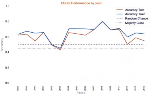
On average, our model outperforms the first two benchmarks in terms of accuracy for the years in our data set as shown in Figure 3.

Model Performance by year

10 - Accuracy Test - Accuracy Train ---- Random Chance 0.8 ••••• M Chs 0.6 0.4 0.2 0.0 Years

Figure 3: Model Accuracy by Year.

Since our data spans the years between 1998 to 2013, it includes economic crisis years 2007-2008. To check if the model performed equally well in somewhat stable economic conditions, we subsequently left out these years from the data and re-trained the Random Forest using the same features. Figure 4 shows that for the the train set, the average accuracy of our model is slightly less that the benchmark gravity model if we include crisis years (4a). However, if we don't include crisis years our model outperforms the benchmark gravity model in most cases(4b) with a significantly smaller variation. For the accuracy on the out of sample data or test set, both models perform very similarly with our model performing only slightly better on average.

Average Model Accuracy Train Set 0.8 07 06 05 0.4 0.3 0.2 0l1 00 our model 0.80 075 070 0.65 0.60 0.56 gevuty

(a) Average accuracy with crisis train set.

Average Model Accuracy (Tram set)

L

0,50#

0.45 0

(b) Average accuracy without crisis train set.

Figure 4: Average Accuracy for training set

This figure shows the average model accuracy on the training data when including or excluding crisis years from the data set.

Average Model Accuracy Test Set 0.80 075 0.70 065 0.60 0.55 050 045 our model

Average Model Accuracy (Tet sel)

0.80 0.75 070 065 060 055 050 045

gavdy our model

(a) Average accuracy with crisis test set (b) Average accuracy without crisis test set

Figure 5: Average Accuracy for test set.

This figure shows the average model accuracy on the test data when including or excluding crisis years from the data set.

5.2

Feature Significance

The significant features for predicting changes in trade identified by Boruta organized in alphabetical order are:

1. Change in GDP A: Changes in the GDP of the source country. The

impor-tance of this feature is expected since a country's ability to export is in part determined by its domestic economy and the state of its productive apparatus.

2. Change in GDP B: Changes in the GDP of the target country. Similarly

to the previous feature, how much trade occurs between any pair of countries will also be in part determined by the ability of the target country to acquire exported goods. We can measure this ability by using the changes in the GDP of the receiving country.

3. Deviation: This feature captures how consistent a particular political

rela-tionship is. That is the degree to which a relarela-tionship is comprised of similarly weighted actions, or is it comprised of very extreme (very cooperative and very conflictive actions).

4. Distance: Distance between the country capitals. This feature is inversely related to the amount of trade between the two countries and is part of the canonical gravity model.

5. GDP Asymmetry: This variable partially captures the power asymmetries

between countries, computed as the difference of GDPs corrected by the source's country's GDP. Since we want to preserve the information about the direction of trade, we don't take the absolute difference and keep the sign. A dyad made up of a developing country exporting goods to a wealthy country has a negative

GDP asymmetry.

6. Max Difference: This variable captures the range of intensity of actions taken

towards the target country in any given year, normalized by the maximum value this feature could take. The maximum difference between Goldstein Scores is 20, for country pairs that have taken extremely cooperative and extremely conflictive actions towards each other. Since this feature is very similar to 'Deviation' we consider it should be removed from future analysis.

7. Mean Goldstein Score (also referred to as Mean): The mean describes

the average 'temperature' or 'intensity' of actions directed towards the target country. As the average of Goldstein scores it can take values between -10 and

10, being -10 the temperature of a very conflictive relationship. The Mean is 32

one of the variables we are most interested in, as it reflects the political and diplomatic relations between the countries in the pair. It includes material and verbal interactions.

8. Verbal Mean: This feature is similar to the previous one, with the difference

that it only includes verbal actions directed towards the target country.

5.3

Feature Importance

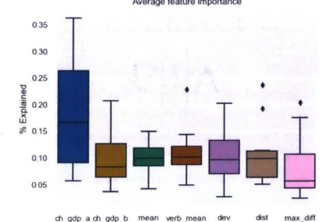
Figure 6 shows the average importance of each feature after aggregating all the MDI importance scores obtained from the yearly models. The most crucial feature for all years is the change in the GDP of the source country. On average it contributes approximately 16% out of the total in each year, but it can explain up to 35% in a given year. Intuitively this result makes sense, mainly because we are using exports, and exports are tightly coupled with the source country's GDP. Together, the changes in GDP for both countries in the dyad explain om average 24-30%.

The mean and the verbal mean follow the changes in GDP in importance. The deviation and distance between countries are next in importance, with the distance performing more consistently than the deviation. Finally, the max difference and verbal interactions are the lowest ranking for MDI importance.

Since the importance of the source country's GDP is larger than most other im-portances, we remove that in Figure 7 to show further detail in the other importances. From plot 7 we notice that on average the importance of the mean and the verbal mean is higher than that of the changes in GDP of the target country. We can also see that on average the importance of the verbal mean is slightly higher that the mean. However, further evidence is needed to be able to assert or quantify the degree to which the two features are interchangeable or if the verbal mean can be used as 'quick and dirty' proxy for the mean. We can also see that the the distribution of importances for the mean and the verbal mean seems to be more narrow than the distribution of distance. Both Mean and Verbal mean seem to have similar or higher importance scores when compared to distance.

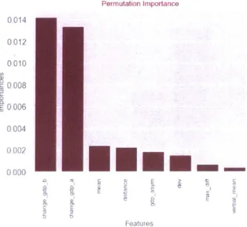
Figure 8 shows the importances as computed using the permutation importance method. Results are similar to results from the MDI method with some differences. First, the GDP of the target country has a higher importance than the one captured with MDI. Accordingly with what we observe from the previous figure, we see that mean and distance seem to have a similar importance, with the mean having a slight advantage.

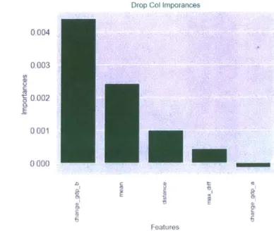
The last method for calculating feature importance reinforces the observations from the past two methods. We show bar plots depicting feature importances using the F1 9 and accuracy score 10 as metrics. Both plots show that the changes in GDPs of the target country are important for model accuracy. With the difference that the GDP of the source country seems to be more important for the F1 metric than for the accuracy score. However, cosnsitently with the previous two methods both the mean stands as one of the top important features. In both cases, the mean is deemed more important than distance.

Average feature importance

0.35 030 0.25 A0.2 w e 0-15

0.10U

005

digdpa

e

gdpb mean verb_mean dev dat max_diff

Figure 6: Feature Importance Boxplot.

This boxplot shows the quarterlies of feature importances calculated using MDI.

Average feature importance

T

4

T

T

dgdpb mean verb_mewn dmv ist maxdiff wfbnt

Figure 7: Feature Importance Boxplot 2

This boxplot shows the quarterlies of feature importances calculated using MDI, without the changes in the GDP of the source country. This boxplot better shows the importances

of other features. Permutation Importance 0014 0012 0010 c 0008 0.006 0.004 0.002 0000

El

C

t

K--> Features

Figure 8: Permutation Importances using accuracy score as target metric. 020 015 'S S

T

0.10

005 1

I I

A I I

Drop Col Imporances 00200 0.0175 0.0150 S0.0125 0.0100 8. 0.0075 0.0050 0.0025 0.0000 Features

Figure 9: Dropping Column Importances with F1 score as target metric.

Drop Col Imporances

0004 0,003 S0002 E 0001 0000 OD 46 Features

Figure 10: Dropping Column Importances with Accuracy score as target metric.

36

6

6

Limitations

The ICEWS data set is biased to include events that are reported by the media. Hence, we cannot recover information about diplomatic interactions that take place in the private sphere between any pair of countries.

Similarly, data about some countries will be underrepresented in our data set. For instance, countries that are not frequently singled out by the media or lead rather uneventful relationships with other countries might not have the same amount of data when compared to more vocal or 'newsworthy' countries like the US. Consequently, certain relationships that originate in some regions of the world like Africa and Latin America will not have less data and might not be included in our analysis.

7

Discussion and Future Work

We build a Random Forest Classifier that predicts changes in exports between country pairs. Our model consistently outperforms two of our benchmarks and performs as well or, in some cases better, than our gravity model benchmark.

We found evidence to that shows that the average intensity of verbal and material political interactions (captured by our feature Mean) are consistently among the top two or three important features for predicting the changes in trade. Our results also suggest that the mean of verbal interactions, as defined by the CAMEO taxonomy, has similar predictive power to the mean. Further work will need to further dive into this result. Finally, our feature importance analysis shows that the intensity of political and diplomatic interactions might be at least as significant as the distance between two countries to predict changes in their trade. In this regard, it might be interesting to measure the importance of distance in time and compare it to the importance of political interactions. Some authors have suggested that political interactions have differential effects on country pairs based on their their income. We did focus on these differential effects, but it seems like a promising avenue for future work. In our work we found that the GDP asymmetry was picked as significant by Boruta. This hints at the possibility that there might be different effects that these scholars are referring to. Yet, it always ranked very low in our importance analysis, thus, we focused on the most relevant features for our analysis.

Bibliography

[1] World trade organization website. https://www.wto.org/english/thewto-e/

whatise/wto_dg_stat_e.htm. Accessed: 2019-08-12.

[2] Olubukola S Adesina. Foreign policy in an era of digital diplomacy. Cogent Social

Sciences, 3(1):1297175, 2017.

13]

ER Afman and M Maurel. Diplomatic relations and trade reorientation in tran-sition countries. Cambridge University Press, 2010.

[4] Mary Ansell. The happy garden. Cassell & co., ltd., 1912.

[51

The Growth Lab at Harvard University. International Trade Data (HS, 92), 2019.

[61

World Bank. https://data.worldbank.org/indicator/ny.gdp.mktp.cd?

view=map. Accessed: 2019-01-11.

171

Nicholas Bayne and Stephen Woolcock. The new economic diplomacy: decision-making and negotiation in international economic relations. Ashgate Publishing,

Ltd., 2011.

[81

Jeffrey H Bergstrand. The gravity equation in international trade: some mi-croeconomic foundations and empirical evidence. The review of economics and

statistics, pages 474-481, 1985.

[91 Corneliu Bjola and Marcus Holmes. Digital diplomacy: Theory and practice. Routledge, 2015.

[10] Elizabeth Boschee, Jennifer Lautenschlager, Sean O'Brien, Steve Shellman,

James Starz, and Michael Ward. ICEWS Coded Event Data, 2015.

[11] Leo Breiman. Random forests. Machine learning, 45(1):5-32, 2001.

[12] Leo Breiman. Manual on setting up, using, and understanding random forests v3. 1. Statistics Department University of California Berkeley, CA, USA, 1:58, 2002.

113]

Maurice JG Bun and Franc Klaassen. The importance of dynamics in panel gravity models of trade. Available at SSRN 306100, 2002.

[14]

Christina L Davis, Andreas Fuchs, and Kristina Johnson. State control and the effects of foreign relations on bilateral trade. Journal of Conflict Resolution, 63(2):405-438, 2019.

[15] Charles De Montesquieu. Montesquieu: The spirit of the laws. Cambridge

Uni-versity Press, 1989.

[16] Representation in Cyprus Directorate-General for Communication. 60

good reasons for the eu. why we need the european union. Avail-able at https://publications.europa.eu/en/publication-detail/-/ publication/f1e5e635-2659-11e7-ab65-0laa75ed7lal/language-en(2017-04-20).

[17] Han Dorussen and Hugh Ward. Trade networks and the kantian peace. Journal

of Peace Research, 47(1):29-42, 2010.

[18] Erik Gartzke. The capitalist peace. American journal of political science,

51(1):166-191, 2007.

[19] Joshua S Goldstein. A conflict-cooperation scale for weis events data. Journal

of Conflict Resolution, 36(2):369-385, 1992.

[20] HAvard Hegre, John R Oneal, and Bruce Russett. Trade does promote peace: New simultaneous estimates of the reciprocal effects of trade and conflict. Journal

of Peace Research, 47(6):763-774, 2010.

121]

Brian Hocking and Jan Melissen. Diplomacy in the digital age. Clingendael, Netherlands Institute of International Relations, 2015.

[22] Matthew 0 Jackson and Stephen Nei. Networks of military alliances, wars, and international trade. Proceedings of the National Academy of Sciences,

112(50):15277-15284, 2015.

[23] Kichun Kang. Overseas network of export promotion agency and export

perfor-mance: the korean case. Contemporary economic policy, 29(2):274-283, 2011. [24] Omar MG Keshk, Brian M Pollins, and Rafael Reuveny. Trade still follows the

flag: The primacy of politics in a simultaneous model of interdependence and armed conflict. The Journal of Politics, 66(4):1155-1179, 2004.

[25] Hyung Min Kim and David L Rousseau. The classical liberals were half right (or

half wrong): New tests of the 'liberal peace', 1960-88. Journal of Peace Research, 42(5):523-543, 2005.

[26] Przemyslaw Kowalski, Max Bige, Monika Sztajerowska, and Matias Egeland.

State-owned enterprises. (147), 2013.

[27] Miron B Kursa, Witold R Rudnicki, et al. Feature selection with the boruta

package. J Stat Softw, 36(11):1-13, 2010. 40

[28] Yonatan Lupu and Vincent A Traag. Trading communities, the networked

struc-ture of international relations, and the kantian peace. Journal of Conflict

Reso-lution, 57(6):1011-1042, 2013.

[29]

Selwyn JV Moons and Peter AG van Bergeijk. Does economic diplomacy work? a meta-analysis of its impact on _{trade and investment. The World Economy,}

40(2):336-368, 2017.

[30] John R Oneal and Bruce Russett. The kantian peace: The pacific benefits of democracy, interdependence, and international organizations, 1885-1992. World

politics, 52(1):1-37, 1999.

[31] John R Oneal and Bruce Russett. Clear and clean: The fixed effects of the liberal peace. International Organization, 55(2):469-485, 2001.

[321

Terence Parr, Kerem Turgutlu, and Jeremy Howard. Beware default random

forest importances. https://explained.ai/rf -importance/index.html. Ac-cessed: 2019-08-12.

[33] Solomon W Polachek, John Robst, and Yuan-Ching Chang. Liberalism and

interdependence: Extending the trade-conflict model. Journal of Peace Research, 36(4):405-422, 1999.

[34]

Andrew K Rose. The foreign service and foreign trade: embassies as export promotion. World Economy, 30(1):22-38, 2007.

135]

Richard N Rosecrance. The rise of the trading state: Commerce and conquest in

the modern world. New York: Basic Books, 1986.

[36] Witold R Rudnicki, Mariusz Wrzesiei, and Wieslaw Paja. All relevant feature

selection methods and applications. In Feature Selection for Data and Pattern

Recognition, pages 11-28. Springer, 2015.

[37] Edward P Stringham. Commerce, markets, and peace: Richard cobden's

endur-ing lessons. The Independent Review, 9(1):105-116, 2004.

[38] Carolin Strobl, Anne-Laure Boulesteix, Achim Zeileis, and Torsten Hothorn.

Bias in random forest variable importance measures: Illustrations, sources and a solution. BMC Bioinformatics, 8(1):25, Jan 2007.

[39] Michael D Ward, Randolph M Siverson, and Xun Cao. Disputes, democracies,

and dependencies: A reexamination of the kantian peace. American Journal of

Political Science, 51(3):583-601, 2007.

140]

Mina Yakop and Peter AG van Bergeijk. Economic diplomacy, trade and devel-oping countries. Cambridge Journal of Regions, Economy and Society,