Demand Forecasting and Inventory Management for Spare Parts

Demand Forecasting and Inventory Management for Spare Parts

by Gaurav Chawla B.E., Mechanical Engineering

Punjab Engineering College, Chandigarh, 2007 M.B.A., Global Logistics and Supply Chain Management SP Jain School of Global Management, Singapore, 2011

and

Vitor Machado Miceli B.E., Industrial Engineering Federal University of Rio de Janeiro, 2013

M.Sc., Business Administration Federal University of Rio de Janeiro, 2015

SUBMITTED TO THE PROGRAM IN SUPPLY CHAIN MANAGEMENT IN PARTIAL FULFILLMENT OF THE REQUIREMENTS FOR THE DEGREE OF

MASTER OF APPLIED SCIENCE IN SUPPLY CHAIN MANAGEMENT AT THE

MASSACHUSETTS INSTITUTE OF TECHNOLOGY JUNE 2019

© 2019 Gaurav Chawla, Vitor Machado Miceli. All rights reserved.

The authors hereby grant MIT permission to reproduce and to distribute publicly paper & electronic copies of this capstone document in whole or in part in any medium now known or hereafter created. Signature of Author: ____________________________________________________________________

Department of Supply Chain Management May 10, 2019 Signature of Author: ____________________________________________________________________ Department of Supply Chain Management

May 10, 2019 Certified by: __________________________________________________________________________ Dr. Nima Kazemi Postdoctoral Associate Capstone Advisor Accepted by: __________________________________________________________________________

Prof. Yossi Sheffi Director, Center for Transportation and Logistics Elisha Gray II Professor of Engineering Systems Professor, Civil and Environmental Engineering

Demand Forecasting and Inventory Management for Spare Parts by

Gaurav Chawla and

Vitor Machado Miceli

Submitted to the Program in Supply Chain Management on May 10, 2019 in Partial Fulfillment of the

Requirements for the Degree of Master of Applied Science in Supply Chain Management ABSTRACT

Spare parts management is an essential operation in the supply chain of many companies, owing to its strategic importance in supporting equipment availability and continuity of operations. In many supply chains, the demand of spare parts is inherently more uncertain compared to traditional fast-moving products. This is due to the fact that spare parts demand is highly intermittent, mostly observed with a long period between consecutive orders, where a no demand period is followed by a period of an order signal. As spare parts are critical to the continuity of operations, companies tend to stock more inventories to mitigate the risk of irregular demand pattern. Gerber Technology, a manufacturing company that sells industrial machines and the spare parts that support them, faces challenges in its spare parts demand forecast quality and inventory management. This challenge has recently been negatively impacting the company’s inventory costs and customer service level, where the actual inventory is consistently higher than the targeted level. Meanwhile, higher inventory levels are not being translated into higher service level to its customers. In summary, the company has seen increased costs with a lower service level. Therefore, the aim of this project was to improve the demand forecast accuracy and the spare parts service level of the company while optimizing inventory costs. For this purpose, we used SKU classification for demand categorization and inventory control. With these categorizations, we then allocate the recommended demand forecasting techniques and optimize the inventory levels of the company. By following these processes, we achieved an improvement between 7% to 14% in forecasting accuracy measured by the Root Mean Squared Error (RMSE). We could also gain up to 3% improvement in service level leading to $1.3M additional revenue opportunity.

Capstone Advisor: Dr. Nima Kazemi Title: Postdoctoral Associate

ACKNOWLEDGMENTS

This project would not have been possible without the kind support and help of many individuals and organizations. We would like to extend our sincere thanks to all of them.

We are specially thankful to Nima Kazemi for his guidance and constant supervision as well as for providing necessary information and support in completing the project.

We would like to express our gratitude towards our families for their kind co-operation and encouragement which help us complete this project.

We would like to express our special gratitude and thanks to Gerber Technology for providing us the opportunity to work in this insightful project and for all their time and attention dedicated to this project. Finally, our thanks and appreciations also go to MIT for making all of this possible and to our colleagues for making part of this great journey.

TABLE OF CONTENTS

LIST OF FIGURES ... 5

LIST OF TABLES ... 5

1 INTRODUCTION ... 6

2 LITERATURE REVIEW ... 8

2.1 SPARE PARTS MANAGEMENT ... 8

2.2 PRODUCT CLASSIFICATION FOR DEMAND FORECASTING ... 9

2.3 DEMAND FORECASTING FOR SPARE PARTS ... 10

2.4 PRODUCT CLASSIFICATION FOR INVENTORY CONTROL ... 11

2.5 CONCLUSION ... 12 3 METHODOLOGY ... 13 3.1 SCOPE ... 13 3.2 ANALYSIS PROCESS ... 13 3.3 DATA COLLECTION ... 16 3.4 SKUCLASSIFICATION ... 17

3.4.1 Classification for Demand Forecasting ... 17

3.4.2 Classification for Inventory Management ... 18

3.5 MODEL ... 21

3.6 OPTIMIZATION TOOL ... 22

4 RESULTS ... 26

4.1 DEMAND PLANNING RESULTS ... 26

4.2 INVENTORY CLASSIFICATION RESULTS ... 31

4.2.1 Comparison with conventional ABC classification: ... 32

4.2.2 Final classification summary ... 33

4.2.3 Impact on Inventory levels, Service Level and Revenue ... 34

5 CONCLUSIONS ... 35

BIBLIOGRAPHY ... 37

LIST OF FIGURES

Figure 1 - Descriptive framework for OR in spare parts management. ... 9

Figure 2- Categorization of different approaches proposed for inventory classification. ... 11

Figure 3 - Analysis Process ... 14

Figure 4 - Demand Classification Categories ... 18

Figure 5 - Demand Classification Categories and Suggested Forecasting Technique ... 18

Figure 6 - Proposed Model for Demand Planning ... 24

Figure 7 - Gerber Inventory Optimization tool: Input Dashboard ... 25

Figure 8 - Gerber Inventory Optimization tool: Output Dashboard ... 25

Figure 9 - SKU Classification Results ... 26

Figure 10 - Percent Forecast Difference in RMSE – Plants 0435 and 0445 ... 28

Figure 11 - Percent Forecast Difference in RMSE – Plants 0446 and 0471 ... 29

Figure 12 - Percent Forecast Difference in RMSE – Plant 0480 ... 29

Figure 13 – Comparison of each group with conventional ABCDS group ... 32

Figure 14 – Number of SKUs that advanced and receded during new classification ... 33

Figure 15 - Final classification of four groups and share of the revenue for each group ... 33

Figure 16 - Impact on inventory levels, Service level and Annual Revenue ... 34

LIST OF TABLES Table 1 – SKU Classification Results ... 26

Table 2 – Proportion of Non-Classified SKU’s per Plant ... 27

Table 3 – Current Forecasting Techniques ... 28

Table 4 – Median Improvement in RMSE ... 30

Table 5 – Negative Performance Analysis ... 31

1 Introduction

The management of spare parts is an important activity for companies in many different sectors (Boylan & Syntetos, 2010). The spare parts category tends to have a higher level of demand uncertainty when compared to traditional fast-moving products, given the nature of the demand itself. Customers only look for the product when the current part is not functioning anymore and this can occur within the lifespan of a machinery, which can last for decades. This demand behavior is reflected and characterized by an intermittent pattern (i.e. long periods of time between two demand signals). Furthermore, given the complex nature and variety of machinery, spare parts tend to have a high number of stock keeping units (SKU's). In addition to the aforementioned factors, the fact that many spare parts are critical to the continuity of operations lead companies to hold higher inventory levels in order to mitigate risk. (Hu, Boylan, Chen, & Labib, 2018).

Gerber Technology is a manufacturing company that designs, sells, and services industrial machines. In addition to the main industrial machines, the company also sells the software that operates them, and the spare parts that support them. The company ships more than 50,000 orders per year into 150 countries to 5,500 customers. More than 10,000 SKUs, coming from 400 vendors, are stored currently in 6 hubs globally (Gerber, 2018). This project will focus on Gerber’s Asian-Pacific region (APAC), which has approximately 3,700 SKU's in its portfolio being stored and delivered to 1,200 customers across its two distribution facilities.

In its spare parts segment, the company faces challenges in its demand forecast quality due to the high uncertainty of customers’ orders, caused by the lack of predictability of order pattern and the fact that a big part of the APAC market is comprised of customers without service contracts. This uncertainty has been negatively impacting the company’s inventory costs in recent years, where the actual inventory is consistently higher than what had been targeted. Meanwhile, higher inventory levels are not being

translated into higher service level to its customers. In summary, the company has seen increased costs with a lower service level.

The goal of this project is to improve the demand forecast accuracy and the spare parts service level of the company while minimizing inventory costs. We will work closely with the on-site team to better understand the business needs, and also to collect the data required to carry out the necessary analysis and develop models. We will use SKU classification for demand categorization and inventory control. With these categorizations, we then allocate the recommended demand forecasting techniques and optimize the inventory levels. By following these processes, we expect to achieve our project goal and also leave a contribution to companies that deal with spare parts items on how to approach them with a step-by-step guide.

2 Literature Review

In this chapter, we begin by explaining how spare parts management differs compared to other types of products. We also discuss studies that explore the framework and guiding steps when dealing with such type of products to create a reference of analysis for the project. Furthermore, we discuss in more detail each part of the process, addressing specifically: (i) product classification for demand forecasting, (ii) demand forecasting for spare parts, and (iii) product classification for inventory control. 2.1 Spare Parts Management

The relevance of the management of spare parts, and its impact on inventory costs among several industries, especially manufacturing, have been discussed in the literature (Gallagher, Mitchke, & Rogers, 2005). The appropriate inventory management is of critical importance in every industry. However, the spare parts segment has two significant particularities that make its management even more challenging: (i) intermittent demand patterns, characterized by sequences of zero demand observations interspersed by occasional and variable non-zero demands (Boylan & Syntetos, 2010), and (ii) the number and variety of spare parts needed to support a single product (Hu et al., 2018).

To better address these characteristics, Hu, Boylan, Chen, & Labib (2018) developed a framework of spare parts management over the lifecycle of the products, highlighting Operations Research (OR) disciplines that support the process. As Figure 1 shows, among the disciplines, the authors suggest in their framework the need to classify every SKU using multicriteria classification techniques that includes two steps: classification for forecasting and classification for inventory control. As a second step, a forecasting technique supported by the classification for each SKU is developed. Finally, the whole portfolio is optimized to satisfy the service level targets with minimal costs (Hu et al., 2018).

Figure 1 - Descriptive framework for OR in spare parts management. Source: Hu, Boylan, Chen, & Labib (2018)

2.2 Product Classification for Demand Forecasting

Williams (1984) was the first to address the categorization of products in order to allocate better demand forecasting techniques for each of the groups. The author used three factors to classify demand: (i) mean number of lead times between demand signals, (ii) a factor of ‘lumpiness’ of demand, and (iii) variation of lead-time. With these factors, the author then classified products in three categories: (i) smooth, (ii) sporadic, and (iii) slow-moving.

A. A. Syntetos (2001) classified demand patterns into four categories: (i) intermittent, (ii) slow-moving, (iii) erratic, and (iv) lumpy by using two factors: (i) average demand interval (ADI), and (ii) square coefficient of variation of demand sizes (CV2_{). The first item is the average time between demand signals} (i.e., how long it takes on average between demand signals appear) whereas the second item is calculated based on the demand signals (i.e., when demand is greater than zero).

Eaves & Kingsman (2004) classified demand in a similar manner, but with a higher level of granularity. In addition to demand variation and the time between demand signals, the authors use the replenishment lead-time as a classification factor. Based on these, five demand patterns emerge (i) smooth, (ii) irregular, (iii) slow-moving, (iv) mildly intermittent, and (v) highly intermittent.

Building upon the previous work, Syntetos, Boylan, & Croston (2005) classified demand for spare parts items in four categories: (i) erratic, (ii) lumpy, (iii) intermittent, and (iv) smooth. The classification was based on the values of the same two factors: (i) squared coefficient of variation, and (ii) average inter-demand interval.

Other classification methods can be found in the literature but the overall objective of demand classification is to identify which demand forecasting technique is more appropriate to be used for each SKU.

2.3 Demand Forecasting for Spare Parts

Forecasting techniques, specifically for spare parts, have its origins with Croston (1972), who argues that significant errors can occur when traditional techniques such as exponential smoothing and moving average are used in the context of intermittent demand, leading to excessive inventory. The author suggests a new algorithm when dealing with such items, taking into consideration the size of the demand when it occurs and the inter-arrival time. It has been shown that the proposed method led to a reduction in forecasting bias and inventory levels for slow-moving items (Croston, 1972).

Syntetos & Boylan (2001) recognized the value of Croston's method when dealing with intermittent demand but showed that the method could lead to only marginal performance gains, or even loss when compared to traditional techniques. The authors then argue that this is due to a mathematical mistake in Croston's derivation and proposed a corrected version of the technique. Then, by using simulation, the authors showed that the updated methods lead to a reduction in forecasting bias.

Others and more complex methods, such as bootstrapping (Zhou & Viswanathan, 2011) are also applied to the context of spare parts demand, showing improvements into specific contexts. However, the industry standard is still considered Croston's method (Hu et al., 2018).

2.4 Product Classification for Inventory Control

Fortuin & Botter (1998) challenged the traditional ABC classification and proposed a new classification called VED (vital, essential and desirable) classification approach that is based on two criteria – functionality and demand rate and furthers develops the stocking strategy based on this classification. Ruud H. Teunter, M. Zied Babai, & Aris A. Syntetos, (2010) proposed an approach for ABC classification that takes into account the demand rate, holding cost, shortage cost, and average order quantity. Millstein, Yang, & Li (2014) proposed a mixed-integer linear programming (MILP) approach to optimize inventory grouping decision based on any desired criteria, including but not limited to, service level targets, inventory spending budget.

Hu, Boylan, Chen & Labib (2018) reviewed different product classification approaches for efficient inventory control that are applied in multiple research papers. The key approaches are summarized in Figure 2.

Figure 2- Categorization of different approaches proposed for inventory classification. Source: Adapted from Hu, Boylan, Chen & Labib (2018)

Classification for Inventory Control

Single Criteria based

classification Multiple Criteria based classification

Fixed no. of classification groups

ABC

Classification ClassificationVED

Optimal no. of classification groups

MILP based grouping

Historically, companies have mainly classified products into A, B and C groups, called ABC classification based on one single criterion – annual cost usage of the spare part, which is calculated as spare part cost multiplied by demand volume (Hu et. Al., 2018). However, many dimensions of spare parts management are ignored while using a single criterion classification.

Other classifications can be found in the literature but the underline conclusion for effective inventory classification for a company is to agree on strategic objectives for inventory management in line with the business strategy that would outline the different criteria for classification thereby defining the final approach for inventory classification.

2.5 Conclusion

The studies presented in this chapter discussed the best practices and concepts that companies should consider when dealing with intermittent items.

In the demand classification area, we decided to follow Syntetos, Boylan, & Croston (2005) approach, since their method was as later corroborated by Van Wingerden, Basten, Dekker, & Rustenburg (2014) as using the most important characteristics (CV2 _{and p) to classify demand.}

In the inventory classification area, we learned through the literature review that none of the papers considers business-oriented parameters in inventory classification. Through our study, we decided to address that gap and by using normalized weighted average approach for multi-criteria inventory classification. This approach enabled us to incorporate both direct parameters like cost of product, revenue potential, and indirect parameters like ship complete, cost of out of stock . This incorporation of parameters captures practical decisions in line with the business strategy.

However, in this study we aim to provide a specific framework that helps companies to manage their demand forecast and inventory of spare part items efficiently. The framework proposes a step-by-step and clear methodology that can be easily adopted by any companies having the same issue in demand forecasting and inventory management.

3 Methodology

In this section, we describe the current forecasting techniques utilized by the company, its current SKU classification, and its inventory management policies. We then propose a model for defining the new SKU classification, in terms of both demand forecasting and inventory management. We also measure the impact of new inventory classification on inventory levels and service level.

The chapter is structured in the following order: (i) definition of the scope of the project, (ii) data collection and analysis, (iii) SKU classification, and (iv) model.

3.1 Scope

As discussed in the introduction section, in addition to its main business line of selling industrial machines and its software, the company also sells the spare parts to support the machine’s operations. This spare parts business has been growing in importance within the company, achieving a relevant position in the revenue share. The Asian-Pacific region (APAC) represents the highest growing market of the spare parts business. However, the cost of this section of the business has also been growing with the increased demand, mainly due to inventory levels. In order to better manage these increasing costs and remain efficient in its spare parts business, the sponsor company wants to achieve this by improving its forecast accuracy for the demand of the spare parts and also optimize its inventory levels. The scope of the project involves finding a forecasting method that is more accurate than the techniques currently used by the company. Moreover, the scope will entail finding the optimal inventory levels. The project is limited to the SKU’s and demand in the APAC region of the company, since they present the most immediate challenges and complexities. Therefore, the other regions that the company operates globally are not analyzed in this study.

3.2 Analysis Process

Figure 3 - Analysis Process

We first identified the company’s current practices. In the case of demand planning, that meant analyzing each forecasting method currently used for each SKU in each plant. For the supply planning side, that meant analyzing the current SKU categorization in terms of A, B, C, D, and S classes. The current forecasting method and SKU categorization techniques established the baseline of our study and this baseline served as the basis when comparing the impacts of the proposed changes.

The second step was improving both the demand and supply planning. For the demand, we classified each SKU in each plant into one of the four demand categories (erratic, lumpy, intermittent, and smooth), and assigned the suggested demand forecasting by the literature review. For the products categorized in the Smooth quadrant, we allocated Croston’s method for the forecast; for all the remaining products we allocated the Syntetos and Boylan Approximation (SBA) method. We used the R package ‘tsintermittent’ to generate both the classification and also the forecasts using the 3-year demand history data.

Finally, we compared the results generated by our model with the baseline. This baseline is defined by what the company is currently using as forecasting method for each product. They are defined by choosing among many different forecasting methods those that generate the least mean absolute percent error (MAPE) in the training set (3-year demand history).

For demand forecasting, the comparison with the current situation was done using the RMSE metric. This error metric is widely used as a standard to asses model performance in many different applications and it also cited in the literature, making it one the most popular error metrics (Chai & Draxler, 2014). This metric is defined by the following equation:

𝑅𝑜𝑜𝑡 𝑀𝑒𝑎𝑛 𝑆𝑞𝑢𝑎𝑟𝑒𝑑 𝐸𝑟𝑟𝑜𝑟 (𝑅𝑀𝑆𝐸) = 2∑>9?@(𝐴𝑐𝑡𝑢𝑎𝑙 𝐷𝑒𝑚𝑎𝑛𝑑9− 𝐹𝑜𝑟𝑒𝑐𝑎𝑠𝑡𝑒𝑑 𝐷𝑒𝑚𝑎𝑛𝑑9)=

𝑁 (1)

We also used the geometric root mean squared error (GRMSE) and mean absolute scaled error (MASE) metrics, defined below, to assess how the new method improved or actually decrease the forecast accuracy based on these metrics. Although not so popular as the RMSE, these are also the error metrics recommended by Syntetos, Boylan, & Croston (2005) when analyzing the results of their forecasting techniques. However, some limitations were found along the way, leaving the final comparison to be done based on the RMSE. These limitations are explained below.

𝐺𝑅𝑀𝑆𝐸 = CD(𝐴𝑐𝑡𝑢𝑎𝑙 𝐷𝑒𝑚𝑎𝑛𝑑9− 𝐹𝑜𝑟𝑒𝑐𝑎𝑠𝑡𝑒𝑑 𝐷𝑒𝑚𝑎𝑛𝑑9)= > 9?@ EF (2) 𝑀𝐴𝑆𝐸 = 1 𝑁∗ I |𝐴𝑐𝑡𝑢𝑎𝑙 𝐷𝑒𝑚𝑎𝑛𝑑9− 𝐹𝑜𝑟𝑒𝑐𝑎𝑠𝑡𝑒𝑑 𝐷𝑒𝑚𝑎𝑛𝑑9| |𝐴𝑐𝑡𝑢𝑎𝑙 𝐷𝑒𝑚𝑎𝑛𝑑₉− 𝑁𝑎𝑖𝑣𝑒 𝐹𝑜𝑟𝑒𝑐𝑎𝑠𝑡𝑒𝑑 𝐷𝑒𝑚𝑎𝑛𝑑₉| > 9?@ (3) Given the multiplicative nature of the GRMSE, any time a specific forecast is correct (i.e. the forecasted demand is equal to the actual demand), the whole series is returned as zero, as if the whole average error was zero. The fact that a zero value would compromise the metric should not pose a problem, since exact forecasts are not common. However, in the current setup of the forecasting system of the company, if a specific forecasting technique is not able to generate forecasts, it will return a series of zeroes instead of generating a series of “not available” values. In this setting, when the future demand is actually zero (very common in the sporadic demand context), the forecasted demand will then be equal

to the actual demand, bringing the whole series to an average of zero, even if errors existed in other points of the forecast. This fact limits the application of this metric and distorts the comparison.

MASE, being a metric calculated over the reference of the errors using a Naïve forecast method, gives a good reference for the performance of the model, but for business purposes, it is more limited than RMSE due to its dimensionless characteristics.

For these reasons, we decided to use the RMSE when reporting the differences in terms of performances, and also because RMSE gives a better parameter to see the impact of the demand forecast improvement in terms of inventory levels.

For the inventory planning, we proposed a multi-criteria inventory classification based on a total of 6 parameters (average unit cost, annual revenue, lead time, ship complete index, cost of out-of-stock, and strategic importance). The first step was to collect the absolute value of each parameter for every SKU. Next, the parameters were classified as direct and indirect parameters and normalized value of each index was calculated for every SKU based on the weight defined for each parameter. Afterwards, the net index value based on the direct and indirect index was calculated and the classification of the SKUs was done based on the number of groups desired. This simulation was done for various combinations of parameters weightage and number of groups to find the best solution in line with business needs and ease of practical implementation. Finally, we measured the impact in expected inventory levels for Gerber for one of the simulation. Using the inventory policy currently used by Gerber, we calculated the change in inventory levels required due to change in classification for every SKU. The expected Service level due to change in inventory was also calculated to estimate the increased revenue opportunity due to improved service level.

3.3 Data Collection

To perform our analysis in the demand planning and supply planning, we needed to gather different types of data. The first collected data was the demand. We collected demand history for every

SKU in every plant of the APAC region for the past three years, which is the period that the company currently uses for demand forecasting purposes. Since the demand data was received in daily level, we had to aggregate the demand data in monthly level to be consistent with the planning period that the company currently uses. Additionally, we gathered the current inventory SKU classification (A, B, C, D, and S) and their respective service levels, the unit cost and price for each SKU in order to evaluate their financial impacts. The last collected data was lead time values – which were given by the company for each product.

3.4 SKU Classification

3.4.1 Classification for Demand Forecasting

The first step in the analysis phase was to classify each spare part commercialized by the company based in its demand pattern. By following Syntetos (2005) approach we classified demand based on two criteria: (i) squared coefficient of variation (CV2_{), and (ii) average inter-demand interval (p). The first item} is calculated based on the demand signals (i.e. when demand is greater than zero), whereas the second item is the average time between demand signals (i.e. how long it takes on average for demand signals to appear). For every SKU, in every single plant, each of these parameters was calculated. Based on their values, the demand pattern was classified into one of four categories: (i) erratic, (ii) lumpy, (iii) intermittent, or (iv) smooth. Demand pattern is said to be erratic if its CV2 _{is greater than 0.49 and its p is} lower or equal to 1.32. For lumpy demand, CV2 _{is greater than 0.49 and p is greater than 1.32. Intermittent} demand is classified by a CV2 _{is lower or equal to 0.49 and p is greater than 1.32. Finally, smooth demand} is classified by a CV2 _{is lower or equal to 0.49 and p is lower or equal to 1.32 (Syntetos, Boylan, & Croston,} 2005). This scheme is summarized by the structure shown in Figure 4.

Figure 4 - Demand Classification Categories Source: Adapted from Syntetos, Boylan, & Croston (2005)

Furthermore, for each of the four quadrants, the authors determined which forecasting method is better suited to it. With the exception of the Smooth quadrant, the SBA is the suggested forecasting method to deal with these types of products. For the Smooth category, Croston’s method is the suggested one. Figure 5 shows the four classifications with their suggested forecasting technique.

Figure 5 - Demand Classification Categories and Suggested Forecasting Technique Source: Adapted from Syntetos, Boylan, & Croston (2005)

3.4.2 Classification for Inventory Management

The first step in inventory management was the classification of the SKUs based on business requirements. As discussed in the literature review, the conventional classification for the SKUs is ABC classification, which is based only on revenue. Using only a single criterion for classification does not serve

Erratic Lumpy Intermittent Smooth Erratic Lumpy Intermittent Smooth

well in spare parts industry because many spare parts are desired to be in stocks not only to provide higher revenue but also to ensure customers will receive their orders (along with other items) without delay. Such business decisions play a major role in inventory classification in the spare parts industry. Therefore, we decided to use multi-criteria inventory classification, which is believed to yield better results as it considers more parameters that impact inventory holding. We considered 6 parameters as defined below: 1. Average Unit Cost (USD): AC

Average unit cost is the standard cost of 1 unit of each product. It includes purchasing cost and logistics cost to bring the item from supplier to Gerber facility. In some cases, the unit cost is in a different currency. The standard exchange rate is then used to convert the price into USD.

2. Annual Revenue (USD): AR

Annual Revenue is the revenue generated by each product in a full year. In other words, it is the number of units sold times the average selling price for each product. If a product is sold free of cost (or complementary with another product), then Annual Revenue can either be assumed as “zero” or equal to the total cost of the product. However, whatever assumption is made, it should be standard across the catalog.

3. Lead Time: LT

Lead time is the planned delivery time in days. It is the time from order to delivery of any product from the supplier facility to the local Gerber facility.

4. Ship Complete: SC

The ship complete criterion is specific to Gerber requirements. Many products (A, B or C class) sometimes wait for a D class product (which is not stocked locally) or vice-a-versa for the shipment to be completed. The unavailability of the product impacts the overall service level if any of the product is not available. Ship complete criterion is defined as the number of orders that include D class SKU divided by total number of orders for each product.

5. Cost of out-of-stock: CO

Cost of out-of-stock is the missed opportunity of selling a product by Gerber when the product is out of stock. Usually, it is the margin of the product unless unavailability of the product also impacts sales of other complementary product. In such cases, the loss of profit from the complementary product is also added in the cost of out-of-stock of the current product.

6. Strategic Importance: SI

Certain products are strategically important and companies. In general, companies tend to store more units to ensure they are never out of stock. The need to have 100% availability can be due to marketing needs, long lead-time or criticality of the product. Strategic importance of a SKU is defined by three numerical values: 1 = low importance, 2 = medium importance, 3 = high importance. By default, all SKUs are considered to be 1.

Direct and Indirect Parameters: To understand how much each of the parameter defined above can influence the classification of each SKU, it is important to know whether the specific parameter impacts the classification directly or indirectly. Hence, we have categorized the 6 parameters into two kinds of parameters: Direct and Indirect Parameter.

The direct parameters are the ones that have a predefined value for each SKU and cannot be manipulated under any circumstances. For example, landed cost of the product cannot change on day to day basis unless product sourcing is changed. AC, AR and LT are defined as direct parameters. The indirect parameters are the ones whose value can be improved or redefined based on the business situation. For example, the strategic importance of an SKU can be high during launch period or peak period and then can be reduced post launch or lean period to ensure the inventory is reduced accordingly. SC, CO and SI are defined as indirect parameters as they do not directly influence the importance of the SKU but can be manually manipulated based on the business decision that can impact their importance. Once the value for each parameter is defined for the full catalogue we run the model as explained in the next section.

3.5 Model

Our proposed model is a combination of all the methods that we gathered in our literature review, but shown in a way that can be applied by managers when dealing with the context of spare parts in case of irregular demand. Figure 6 shows workflow in the context of the demand planning.

For inventory management, the direct index and indirect index are calculated using the values of the 6 parameters defined in section 3.4.2 for every SKU.

𝐷𝑖𝑟𝑒𝑐𝑡 𝐼𝑛𝑑𝑒𝑥 = O_{𝐴𝑣𝑔(𝐴𝐶)}𝐴𝐶 R ∗ 𝑊(𝐴𝐶) + O 𝐴𝑅 𝐴𝑣𝑔(𝐴𝑅)R ∗ 𝑊(𝐴𝑅) + O 𝐿𝑇 𝐴𝑣𝑔(𝐿𝑇)R ∗ 𝑊(𝐿𝑇) (4) 𝐼𝑛𝑑𝑖𝑟𝑒𝑐𝑡 𝐼𝑛𝑑𝑒𝑥 = O_{𝐴𝑣𝑔(𝑆𝐶)}𝑆𝐶 R ∗ 𝑊(𝑆𝐶) + O 𝐶𝑂 𝐴𝑣𝑔(𝐶𝑂)R ∗ 𝑊(𝐶𝑂) + O 𝑆𝐼 𝐴𝑣𝑔(𝑆𝐼)R ∗ 𝑊(𝑆𝐼) (5) 𝑁𝑒𝑡 𝐼𝑛𝑑𝑒𝑥 = 𝐷𝑖𝑟𝑒𝑐𝑡 𝐼𝑛𝑑𝑒𝑥 + 𝐼𝑛𝑑𝑖𝑟𝑒𝑐𝑡 𝐼𝑛𝑑𝑒𝑥 (6) where:

AC, AR, LT, SC, CO, SI are the parameters as defined in section 3.4.2 𝐴𝑣𝑔(𝑥) = Average of parameter ‘x’ across the catalogue

𝑊(𝑥) = Weighted percentage of parameter ‘x’

Once the direct index and indirect index are calculated, the net index is calculated as the sum of the two indexes. The reason we calculated the direct index and indirect index separately is to understand the impact of direct and indirect parameters on the net index. Once the net index is calculated for each SKU, the catalog is classified into the desired number of groups based on the cutoff percentage set for each group.

To be able to generate a multi-criteria inventory classification in different settings, we have developed a simulation tool using Visual Basic that provides the classification of the SKUs based on the inputs entered by the user. The step by step explanation of each element of the tool is explained in the next section.

3.6 Optimization Tool

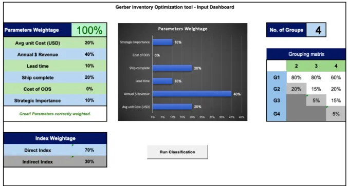
Figure 7 shows a typical dashboard of the model for inventory classification. The explanation of each lever is as below:

§ Parameters Weightage

This table includes all the parameters discussed in 3.4.2. The user needs to provide the weight for each parameter. If the sum of the provided weight is not 100%, the tool will prompt the user to correct and adjust the values to meet 100%.

§ Index Weightage

The Index Weightage table shows the split between the direct and indirect indexes. The direct index incorporated all the direct parameters while the indirect index incorporated all the indirect parameters as defined in section 3.4.2. The index value for each SKU is calculated based on the sum product of the deviation of each parameter from the mean and the weight of each parameter as input by the user.

§ No. of Groups

This table requires the desired number of groups in which the inventory need to be classified. This ranges from 1 to 4.

§ Grouping matrix

Grouping matrix defines the cut off cumulative percentage for each group based on a cumulative net index. This can be manually adjusted as per business decisions.

Once the parameters are set, the model is run to assign a group number to each SKU based on input parameters. The modeling is done in VBA and the code is provided in the Appendix section.

Based on the new classification, we then compared the shift of SKUs from lower class in old classification (ABCDS) to higher class in new classification (G1, G2, G3, G4) and vice versa. This shift of SKUs from one class to another will have both positive and negative impact on inventory levels. Hence,

the net impact on inventory will depend on the input parameters chosen for the classification and the extent of shift of SKUs from one class to another. We used the current R,S policy as used by Gerber to calculate the net inventory requirement, however the model provides the flexibility to set different service level targets for each group to finally calculate the total inventory requirement and overall service level expected. The results of one such simulation are provided in the Results section.

Figure 7 - Gerber Inventory Optimization tool: Input Dashboard

4 Results

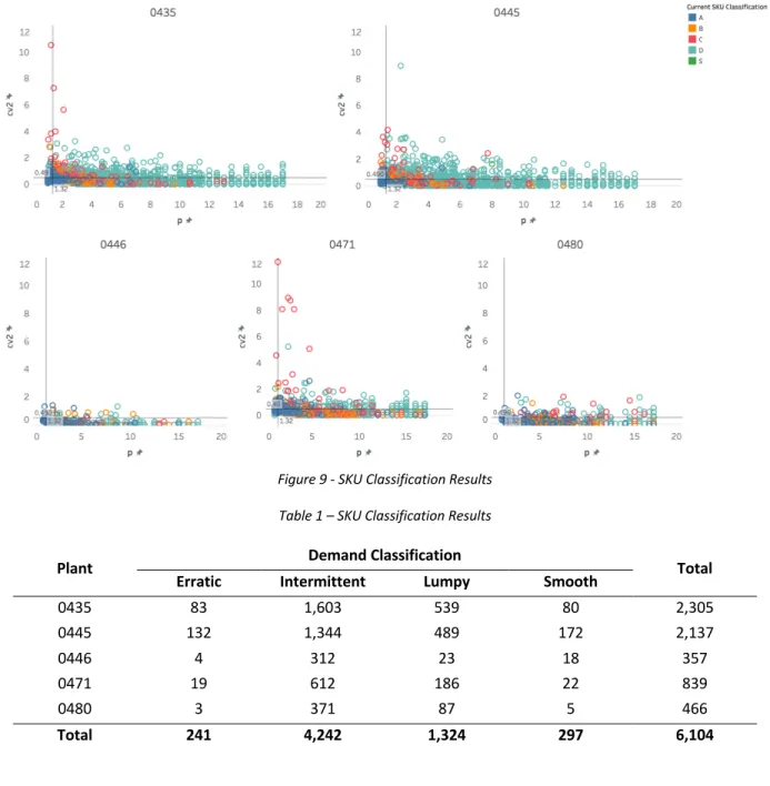
Figure 6, the first step in our process was to analyze the company’s portfolio of production at each of their plants and classify them accordingly for demand forecast purposes. Figure 9 shows graphically the final results of this classification step for each company’s plant that actually holds inventory and therefore it is impacted by the demand forecast. Table 1 summarizes these values.

Figure 9 - SKU Classification Results Table 1 – SKU Classification Results

Plant Demand Classification Total

Erratic Intermittent Lumpy Smooth

0435 83 1,603 539 80 2,305 0445 132 1,344 489 172 2,137 0446 4 312 23 18 357 0471 19 612 186 22 839 0480 3 371 87 5 466 Total 241 4,242 1,324 297 6,104

Most of the SKU’s were classified in the intermittent or lumpy category, with fewer occurrences in the smooth and erratic categories, showing the complexity that the company faces regarding the demand pattern for their spare parts business.

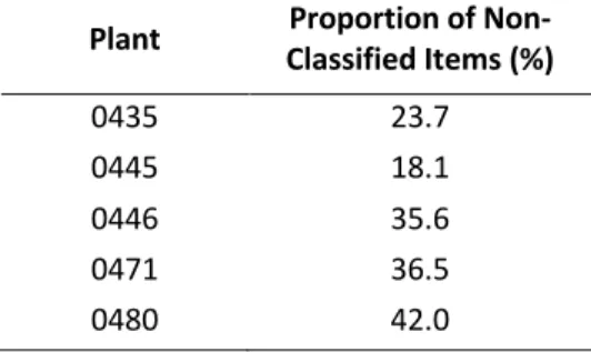
Moreover, many products were not classified in one of the four categories since they did not have enough demand signals in the past 3 years. Table 2 summarizes the proportion of SKU’s per each plant that was not able to be classified (i.e. did not have at least two demand signals over the past 3 years):

Table 2 – Proportion of Non-Classified SKU’s per Plant

Plant _{Classified Items (%)} Proportion of

Non-0435 23.7

0445 18.1

0446 35.6

0471 36.5

0480 42.0

Since the company works with a monthly forecast period, our classification took this fact into account and we grouped all the demand data for each SKU and plant into monthly periods. If one particular SKU in a particular plant had an order in only one month or did not have an order at all, we were not able to classify it. This non-classification happens because at least two demand signals are required to calculate an average inter-demand interval (p). Furthermore, this is the reason we do not see any plant with the number of 3,703 SKU’s initially mentioned (which is the number of unique active products in the company). Moreover, not all products are commercialized in all plants.

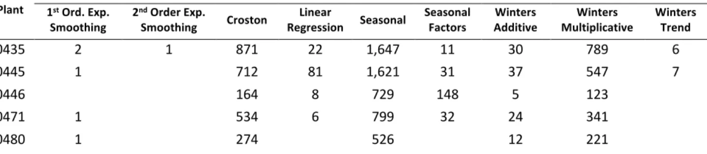
Table 3 summarizes the current forecasting techniques used currently by the company. Table 3 – Current Forecasting Techniques

Plant Forecast Procedures 1st _{Ord. Exp.} Smoothing 2nd _{Order Exp.} Smoothing Croston Linear Regression Seasonal Seasonal Factors Winters Additive Winters Multiplicative Winters Trend 0435 2 1 871 22 1,647 11 30 789 6 0445 1 712 81 1,621 31 37 547 7 0446 164 8 729 148 5 123 0471 1 534 6 799 32 24 341 0480 1 274 526 12 221

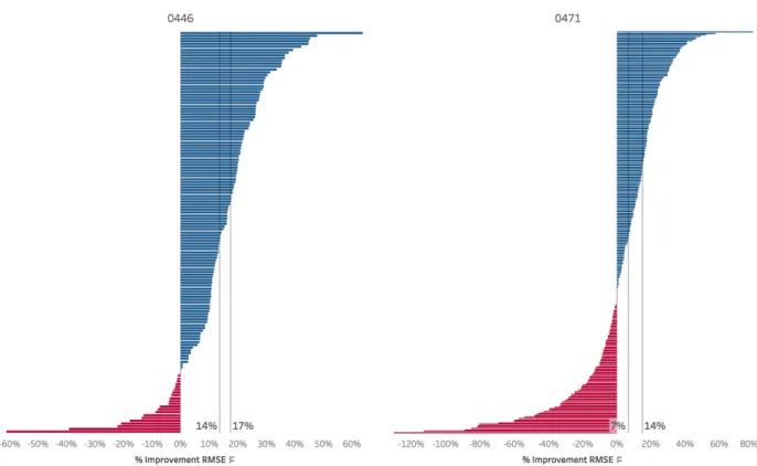
Figure 10 to 12 shows the relative difference in percent terms of the proposed methods over the baseline forecasting techniques. Blue bars indicate a positive improvement (i.e. lower RMSE) and red bars indicate negative performance (i.e. higher RMSE).

Figure 11 - Percent Forecast Difference in RMSE – Plants 0446 and 0471

Figure 12 - Percent Forecast Difference in RMSE – Plant 0480

As can be seen from the graphs, the overall results are an increase in forecast accuracy in every plant measured by the RMSE when using the suggested forecasting methods. However, there are still many SKUs that actually have their accuracy worsened when changing the current forecasting technique to the suggested. To this reason, we aggregated the results in two ways: (i) calculating the median improvement in RMSE using all SKUs, and (ii) calculating the median improvement in RMSE using only SKUs that actually had a better forecast. Table 4 summarizes these results:

Table 4 – Median Improvement in RMSE

Plant Median Improvement RMSE – Positive Cases Median Improvement RMSE – All Cases

0435 15% 13%

0445 13% 10%

0446 17% 14%

0471 14% 7%

0480 17% 11%

As can be seen, by following the classification method for demand and the suggested forecasting technique for each SKU, we were able to increase the forecasting accuracy in the range of 7% to 14% in the plants. If we account only for the positive cases (i.e. don’t change the forecast method if the current performs better), we see a median improvement range of 13%-17%. This can potentially represent a direct impact on the company’s safety stock value, depending on the value of each product and its improved accuracy.

However, as mentioned earlier, we still had some cases of items that had its accuracy worsened. To understand where most of these cases are happening, we analyzed the relative amount of these cases by SKU category (A, B, C, D, and S) and by demand classification (Erratic, Intermittent, Lumpy, and Smooth). Table 5 summarizes these findings:

Table 5 – Negative Performance Analysis

SKU Category

Demand Classification

Total Erratic Intermittent Lumpy Smooth

A 4% 11% 5% 8% 28%

B 1% 12% 5% 1% 19%

C 2% 25% 20% 1% 47%

S 5% 1% 0% 6%

We can see that most cases are happening within the C category and within the Intermittent and Lumpy categories. These results are reasonable given the fact that the Intermittent and Lumpy category are the ones with a higher period of time between demand signals, making its prediction challenging. Furthermore, on the business side, it is best that most of these cases are happening in the C category, due to its lower relative value of products compared to the other categories.

4.2 Inventory Classification Results

Once the optimization model is successfully run, the final grouping of the SKUs is generated. The new groups are classified as G1, G2, G3, G4 (as against ABCD in conventional classification) in the order where G1 represents the most important SKUs and G4 represents the least important SKUs. Figure 8 shows the typical output dashboard of the model. The results are measured in 3 categories:

1) Shift of SKUs to higher or lower classification vs conventional ABC classification (Fig 13) 2) Share of revenue by each group in new classification

4.2.1 Comparison with conventional ABC classification:

Figure 13 – Comparison of each group with conventional ABCDS group

Figure 13 compares the conventional ABC with model output (G1, G2, G3, G4). Most of the SKUs that were previously classified as A class fall under G1 category. This is expected as the A class SKUs are clearly the most important SKUs in terms of revenue generation and inventory management. However, we also noticed 341 SKUs, previously classified as D class, are now proposed by the model under G1 group. These are the SKUs that despite being small in revenue generation, have a big impact on service level due to other parameters like ship complete as explained in section 3.4.2. For instance, a D class SKU needs to be shipped together with A class SKU, if out of stock impacts the service level of A class SKU as well.

Table 6 – Conventional vs New Classification matrix

Conventional Classification New Classification G1 G2 G3 G4 A 166 18 1 1 B 109 140 21 7 C 15 73 200 87 D 341 665 769 293 S 2 3 7 6

Table 6 compares the matrix of conventional classification the new highlighted in green are the ones whose class was advanced and the cells highlighted in red are the ones whose class was receded. The movement of D class SKUs is highlighted as all D class SKUs were not stocked by default in the

166 18 _{1 1} 109 140 21 ₇ 15 73 200 87 341 665 769 293 2 3 7 6 G1 G2 G3 G4

COMPARISON VS CONVENTIONAL ABC

Figure 14 – Number of SKUs that advanced and receded during new classification

Considering ABC classes only, 197 SKUs were proposed to be in higher class while 135 SKUs were proposed to be in a lower class than before (ref. Figure 14). This is due to the influences of parameters other than revenue (refer to Section 3.4.2).

4.2.2 Final classification summary

Figure 15 - Final classification of four groups and share of the revenue for each group

Figure 15 shows the number and percentage of SKUs grouped under each group and a corresponding share of the revenue. 88% of revenue is covered by 22% of SKUs classified as G1. Hence, it makes sense to only focus on G1 and G2 in terms of inventory management as they contribute to almost 98% of revenue. Almost half of the catalog (47%) falls under G3 and G4 that only contribute to 2% of the revenue. Hence, service level requirement need not be very stringent for these groups.

197

SKUs

SKUs

135

Class r

ece

de

d

4.2.3 Impact on Inventory levels, Service Level and Revenue

Figure 16 - Impact on inventory levels, Service level and Annual Revenue

Figure 16 shows the impact on inventory levels, service level and annual revenue with the new classification. We observe an increase in inventory by $271K mainly driven by D class SKUs which were previously not stocked at all. However, the increase in inventory is justified by the expected gain in service level and hence revenue. We expect an improved of approx. 3% in Service level with additional revenue opportunity of $1.3M with the improved service level.

$235 $1,201 $36 $150 $ $200 $400 $600 $800 $1,000 $1,200 $1,400 $1,600 Increase in Inventory Annual Gain in Revenue Th ou sa nd s Impact on inventory and expected revenue with improvement in Service Level D Class ABCS Class 55% 88.80% _86% 84.90% 89.10% 89% 0% 10% 20% 30% 40% 50% 60% 70% 80% 90% 100%

D Class ABCS Class Total

Improvement in Service Level for ABCDS class SKUs

5 Conclusions

In this project, we researched the literature to find best practices for companies when dealing with the scope of managing spare parts. In this research, we focused on main topics that companies have to address in this context. The first one is with regards to their demand forecasting practices and the second one is with regards to their inventory management practices.

Within the demand forecasting scope, we followed the recommendations provided by Syntetos, Boylan, & Croston (2005). The recommendation is based on the classification of each SKU into four categories and allocating the appropriate forecasting method to the respective classification.

Within the inventory management scope, we followd the multi-criteria inventory classification and used normalized weighted average approach to incorporate the business priorities in inventory planning. The final deliverable in inventory management is the optimization tool that simulates the inventory planning based on different inputs and provides the new classification for the SKUs for inventory holding. The tool also measures impact on inventory level, service level and revenue in different scenarios.

By following the described method, we were able to improve the forecast accuracy in RMSE terms for the company’s plants in the range of 7% to 14%, which is reflected in a reduction of the company’s safety stock.

Furthermore, by changing the inventory classification method, we were able to improve the service level by 3% leading to an additional revenue opportunity of approximately $1.3M with the current demand pattern. The inventory mix will change due to the shift of SKUs from one class to another, however this would improve the overall quality of inventory and help in better service level and inventory management. Although the new inventory classification proposed an increase in inventory, driven mainly by D class SKUs that were not previously stocked, the net impact on inventory, with the implementation of both demand planning and supply planning recommendations, is expected to be favorable.

We recommend Gerber to do a pilot study with the new forecasting method of the proposed SKUs and new inventory classification of key SKUs and measure the impact of the same on business. Furthermore, using the optimization tool with different business scenarios (and values for indirect parameters for key SKUs) would also help to get more accurate results in line with business needs.

BIBLIOGRAPHY

Boylan, J. E., & Syntetos, A. A. (2010). Spare parts management: A review of forecasting research and extensions. IMA Journal of Management Mathematics, 21(3), 227–237.

Chai, T., & Draxler, R. R. (2014). Root mean square error (RMSE) or mean absolute error (MAE)? -Arguments against avoiding RMSE in the literature. Geoscientific Model Development, 7(3), 1247– 1250.

Croston, J. D. (1972). Forecasting and Stock Control for Intermittent Demands. Journal of the

Operational Research Society, 23(3), 289–303.

Eaves, A. H. C., & Kingsman, B. G. (2004). Forecasting for the ordering and stock-holding of spare parts,

Journal of the Operational Research Society, . 55, 431–437.

Fortuin, L., & Botter, R. (1998). Stocking strategy for service parts - a case study. International Journal of

Operations & Production Management, 33.

Gallagher, T., Mitchke, M. D., & Rogers, M. C. (2005). Profiting from spare parts. The McKinsey Quarterly,

2(Exhibit 2), 1–4.

Gerber. (2018). No Title.

Hu, Q., Boylan, J. E., Chen, H., & Labib, A. (2018). OR in spare parts management: A review. European

Journal of Operational Research, 266(2), 395–414.

Millstein, M. A., Yang, L., & Li, H. (2014). Optimizing ABC inventory grouping decisions. International

Journal of Production Economics, 148, 71–80.

Ruud H. Teunter, M. Zied Babai, & Aris A. Syntetos. (2010). ABC Classification: Service Levels and Inventory Costs. Production and Operations Management, 19(3), 343–354.

Syntetos, A. A. (2001). Forecasting of intermittent demand. Dissertation, 1–495.

Syntetos, A. A., Boylan, J. E., & Croston, J. D. (2005). On the categorization of demand patterns. Journal

of the Operational Research Society, 56(5), 495–503.

Syntetos, A., & Boylan, J. E. (2001). On the bias of intermittent demand estimates. International Journal

of Production Economics, 71(2), 457–466.

Van Wingerden, E., Basten, R. J. I., Dekker, R., & Rustenburg, W. D. (2014). More grip on inventory control through improved forecasting: A comparative study at three companies. International

Journal of Production Economics, 157(1), 220–237.

Williams, T. M. (1984). Stock Control with Sporadic and Slow-Moving Demand. Journal of the

Operational Research Society, 35(10), 939–948. Retrieved from

Zhou, C., & Viswanathan, S. (2011). Comparison of a new bootstrapping method with parametric

approaches for safety stock determination in service parts inventory systems. International Journal

APPENDIX A

Visual Basic Code for the model:

Sub Grouping()

'' This code does the grouping based on input parameters '' Keyboard Shortcut: Option+Cmd+g

' Sheets("Classification").Select Cells.Select Selection.Delete Worksheets("Dashboard").Range("B6:C12").Copy Worksheets("Classification").Range("B3").PasteSpecial Paste:=xlPasteValues Sheets("Dashboard").Select Range("B17:C19").Select Application.CutCopyMode = False Selection.Copy Sheets("Classification").Select Range("E3").Select

Selection.PasteSpecial Paste:=xlValues, Operation:=xlNone, SkipBlanks:= _ False, Transpose:=False

Sheets("Dashboard").Select Range("L6:N6").Select Application.CutCopyMode = False Selection.Copy Sheets("Classification").Select Range("H3").Select

Selection.PasteSpecial Paste:=xlValues, Operation:=xlNone, SkipBlanks:= _ False, Transpose:=False

Sheets("Data").Select Worksheets("Data").Range("B4:D2928,N4:N2928").Copy Worksheets("Classification").Range("B13").PasteSpecial Paste:=xlPasteValues Sheets("Classification").Select Application.CutCopyMode = False ActiveWorkbook.Worksheets("Classification").Sort.SortFields.Clear ActiveWorkbook.Worksheets("Classification").Sort.SortFields.Add Key:=Range("E14:E2938") _ , SortOn:=xlSortOnValues, Order:=xlDescending, DataOption:=xlSortNormal

With ActiveWorkbook.Worksheets("Classification").Sort .SetRange Range("B13:E2938") .Header = xlYes .MatchCase = False .Orientation = xlTopToBottom .SortMethod = xlPinYin .Apply EndWith Sheets("Classification").Select Range("F13").Select

ActiveCell.FormulaR1C1 = "Cumulitive %age" Range("F14").Select ActiveCell.FormulaR1C1 = "=RC[-1]/SUM(C[-1])" Range("F15").Select ActiveCell.FormulaR1C1 = "=R[-1]C+RC[-1]/SUM(C[-1])" Range("F15").Select Selection.AutoFill Destination:=Range("F15:F2938") Range("F15:F2938").Select Sheets("Classification").Select Range("G13").Select ActiveCell.FormulaR1C1 = "Groups" Range("G14").Select ActiveCell.FormulaR1C1 = "=IF(R3C10=2,IF(RC[-1]<=Dashboard!R10C13,""G1"",""G2""),IF(R3C10=3,IF(RC[-

1]<=Dashboard!R10C14,""G1"",IF(RC[-1]>(Dashboard!R10C14+Dashboard!R11C14),""G3"",""G2"")),IF(R3C10=4,IF(RC[- 1]<=Dashboard!R10C15,""G1"",IF(AND(RC[-1]>Dashboard!R10C15,RC[-1]<=(Dashboard!R10C15+Dashboard!R11C15)),""G2"",IF(RC[-1]>SUM(Dashboard!R10C15:R12C15),""G4"",""G3""))))))" Range("G14").Select Selection.AutoFill Destination:=Range("G14:G2938") Range("G14:G2938").Select Sheets("Classification").Select Range("B2").Select

ActiveCell.FormulaR1C1 = "Simulation Parameters" Range("B2").Select Selection.Font.Bold = True ExecuteExcel4Macro "PATTERNS(1,0,9,TRUE,2,4,0,0.399975585192419)" Selection.Font.Size = 16 Range("B2:J2").Select With Selection .HorizontalAlignment = xlCenter .VerticalAlignment = xlBottom .WrapText = False .Orientation = 0 .AddIndent = False .ShrinkToFit = False .MergeCells = False EndWith Selection.Merge Range("B2:J9").Select Selection.Borders(xlDiagonalDown).LineStyle = xlNone Selection.Borders(xlDiagonalUp).LineStyle = xlNone With Selection.Borders(xlEdgeLeft) .LineStyle = xlContinuous .Weight = xlMedium .ColorIndex = xlAutomatic EndWith With Selection.Borders(xlEdgeTop) .LineStyle = xlContinuous .Weight = xlMedium .ColorIndex = xlAutomatic EndWith With Selection.Borders(xlEdgeBottom) .LineStyle = xlContinuous .Weight = xlMedium .ColorIndex = xlAutomatic EndWith With Selection.Borders(xlEdgeRight) .LineStyle = xlContinuous .Weight = xlMedium .ColorIndex = xlAutomatic EndWith Selection.Borders(xlInsideVertical).LineStyle = xlNone Selection.Borders(xlInsideHorizontal).LineStyle = xlNone Range("B13:G13").Select Selection.Font.Bold = True ExecuteExcel4Macro "PATTERNS(1,0,9,TRUE,2,4,0,0.399975585192419)" Selection.Font.Size = 16 Columns("B:G").Select Columns("B:G").EntireColumn.AutoFit Range("B13:G2938").Select Selection.Borders(xlDiagonalDown).LineStyle = xlNone Selection.Borders(xlDiagonalUp).LineStyle = xlNone With Selection.Borders(xlEdgeLeft) .LineStyle = xlContinuous .Weight = xlMedium .ColorIndex = xlAutomatic EndWith

With Selection.Borders(xlEdgeTop) .LineStyle = xlContinuous .Weight = xlMedium .ColorIndex = xlAutomatic EndWith With Selection.Borders(xlEdgeBottom) .LineStyle = xlContinuous .Weight = xlMedium .ColorIndex = xlAutomatic EndWith With Selection.Borders(xlEdgeRight) .LineStyle = xlContinuous .Weight = xlMedium .ColorIndex = xlAutomatic EndWith Selection.Borders(xlInsideVertical).LineStyle = xlNone Selection.Borders(xlInsideHorizontal).LineStyle = xlNone Range("I22").Select ActiveCell.FormulaR1C1 = "Summary" Range("I23").Select ActiveCell.FormulaR1C1 = "Group" Range("J23").Select

ActiveCell.FormulaR1C1 = "No. of SKUs" Range("I24").Select ActiveCell.FormulaR1C1 = "G1" Range("I25").Select ActiveCell.FormulaR1C1 = "G2" Range("I26").Select ActiveCell.FormulaR1C1 = "G3" Range("I27").Select ActiveCell.FormulaR1C1 = "G4" Range("J24").Select ActiveCell.FormulaR1C1 = "=COUNTIF(C[-3],RC[-1])" Range("J24").Select

Selection.AutoFill Destination:=Range("J24:J27"), Type:=xlFillDefault Range("J24:J27").Select Range("I22").Select ExecuteExcel4Macro "PATTERNS(1,0,9,TRUE,2,4,0,0.399975585192419)" Selection.Font.Bold = True Selection.Font.Size = 16 Range("I22:J27").Select Selection.Borders(xlDiagonalDown).LineStyle = xlNone Selection.Borders(xlDiagonalUp).LineStyle = xlNone With Selection.Borders(xlEdgeLeft) .LineStyle = xlContinuous .Weight = xlMedium .ColorIndex = xlAutomatic EndWith With Selection.Borders(xlEdgeTop) .LineStyle = xlContinuous .Weight = xlMedium .ColorIndex = xlAutomatic EndWith With Selection.Borders(xlEdgeBottom) .LineStyle = xlContinuous .Weight = xlMedium .ColorIndex = xlAutomatic EndWith With Selection.Borders(xlEdgeRight) .LineStyle = xlContinuous .Weight = xlMedium

EndWith Selection.Borders(xlInsideVertical).LineStyle = xlNone Selection.Borders(xlInsideHorizontal).LineStyle = xlNone Range("I22:J22").Select With Selection .HorizontalAlignment = xlCenter .VerticalAlignment = xlBottom .WrapText = False .Orientation = 0 .AddIndent = False .ShrinkToFit = False .MergeCells = False EndWith Selection.Merge Range("I23:J27").Select With Selection .HorizontalAlignment = xlLeft .VerticalAlignment = xlBottom .WrapText = False .Orientation = 0 .AddIndent = False .IndentLevel = 0 .ShrinkToFit = False .MergeCells = False EndWith With Selection .HorizontalAlignment = xlCenter .VerticalAlignment = xlBottom .WrapText = False .Orientation = 0 .AddIndent = False .ShrinkToFit = False .MergeCells = False EndWith Range("I23:J23").Select Selection.Font.Bold = True Sheets("Dashboard").Select Range("AA14").Select ActiveCell.FormulaR1C1 = "=Classification!R[10]C[-17]" Sheets("Dashboard").Select Range("AA15").Select ActiveCell.FormulaR1C1 = "=Classification!R[10]C[-17]" Sheets("Dashboard").Select Range("AA16").Select ActiveCell.FormulaR1C1 = "=Classification!R[10]C[-17]" Sheets("Dashboard").Select Range("AA17").Select ActiveCell.FormulaR1C1 = "=Classification!R[10]C[-17]" Sheets("Dashboard").Select Sheets("Dashboard").Select Range("AD14").Select ActiveCell.FormulaR1C1 = _ "=COUNTIFS(Classification!C7,Dashboard!RC29,Classification!C4,Dashboard!R13C)" Range("AE14").Select ActiveCell.FormulaR1C1 = _ "=COUNTIFS(Classification!C7,Dashboard!RC29,Classification!C4,Dashboard!R13C)" Range("AF14").Select ActiveCell.FormulaR1C1 = _ "=COUNTIFS(Classification!C7,Dashboard!RC29,Classification!C4,Dashboard!R13C)" Range("AG14").Select ActiveCell.FormulaR1C1 = _ "=COUNTIFS(Classification!C7,Dashboard!RC29,Classification!C4,Dashboard!R13C)"

Range("AH14").Select ActiveCell.FormulaR1C1 = _ "=COUNTIFS(Classification!C7,Dashboard!RC29,Classification!C4,Dashboard!R13C)" Range("AD15").Select ActiveCell.FormulaR1C1 = _ "=COUNTIFS(Classification!C7,Dashboard!RC29,Classification!C4,Dashboard!R13C)" Range("AE15").Select ActiveCell.FormulaR1C1 = _ "=COUNTIFS(Classification!C7,Dashboard!RC29,Classification!C4,Dashboard!R13C)" Range("AF15").Select ActiveCell.FormulaR1C1 = _ "=COUNTIFS(Classification!C7,Dashboard!RC29,Classification!C4,Dashboard!R13C)" Range("AG15").Select ActiveCell.FormulaR1C1 = _ "=COUNTIFS(Classification!C7,Dashboard!RC29,Classification!C4,Dashboard!R13C)" Range("AH15").Select ActiveCell.FormulaR1C1 = _ "=COUNTIFS(Classification!C7,Dashboard!RC29,Classification!C4,Dashboard!R13C)" Range("AD16").Select ActiveCell.FormulaR1C1 = _ "=COUNTIFS(Classification!C7,Dashboard!RC29,Classification!C4,Dashboard!R13C)" Range("AE16").Select ActiveCell.FormulaR1C1 = _ "=COUNTIFS(Classification!C7,Dashboard!RC29,Classification!C4,Dashboard!R13C)" Range("AF16").Select ActiveCell.FormulaR1C1 = _ "=COUNTIFS(Classification!C7,Dashboard!RC29,Classification!C4,Dashboard!R13C)" Range("AG16").Select ActiveCell.FormulaR1C1 = _ "=COUNTIFS(Classification!C7,Dashboard!RC29,Classification!C4,Dashboard!R13C)" Range("AH16").Select ActiveCell.FormulaR1C1 = _ "=COUNTIFS(Classification!C7,Dashboard!RC29,Classification!C4,Dashboard!R13C)" Range("AD17").Select ActiveCell.FormulaR1C1 = _ "=COUNTIFS(Classification!C7,Dashboard!RC29,Classification!C4,Dashboard!R13C)" Range("AE17").Select ActiveCell.FormulaR1C1 = _ "=COUNTIFS(Classification!C7,Dashboard!RC29,Classification!C4,Dashboard!R13C)" Range("AF17").Select ActiveCell.FormulaR1C1 = _ "=COUNTIFS(Classification!C7,Dashboard!RC29,Classification!C4,Dashboard!R13C)" Range("AG17").Select ActiveCell.FormulaR1C1 = _ "=COUNTIFS(Classification!C7,Dashboard!RC29,Classification!C4,Dashboard!R13C)" Range("AH17").Select ActiveCell.FormulaR1C1 = _ "=COUNTIFS(Classification!C7,Dashboard!RC29,Classification!C4,Dashboard!R13C)" Range("A61").Select EndSub