Demand Uncensored:
Car-Sharing Mobility Services Using Data-Driven
and Simulation-Based Techniques
by
Evan Fields
B.A., Pomona College (2013)
Submitted to the Sloan School of Management
in partial fulfillment of the requirements for the degree of Doctor of Philosophy in Operations Research
at the
MASSACHUSETTS INSTITUTE OF TECHNOLOGY February 2019
Massachusetts Institute of Technology 2019. All rights reserved.
Signature redacted
A uthor ...Sloanqchool of Management September 14, 2018
Certified by
...
Signature
redacted
Carolina Osorio Associate Professor hesis Supervisor
Signature
redacted-A ccepted by ... ...
MASSACHUSETTS INSTITUTE k.D itris Bertsimas OFTEHNOG Boeing Professor of Operations Research
MAR
1,6 2019
Co-Director, Operations Research CenterLIBRARIES
ARCHIVES
Demand Uncensored: Inferring Demand for Car-Sharing
Mobility Services Using Data-Driven and Simulation-Based
Techniques
by
Evan Fields
Submitted to the Sloan School of Management on September 14, 2018, in partial fulfillment of the
requirements for the degree of
Doctor of Philosophy in Operations Research
Abstract
In the design and operation of urban mobility systems, it is often desirable to un-derstand patterns in traveler demand. However, demand is typically unobserved and must be estimated from available data. To address this disconnect, we begin by proposing a method for recovering an unknown probability distribution given a cen-sored or truncated sample from that distribution. The proposed method is a novel and conceptually simple detruncation technique based on sampling the observed data according to weights learned by solving a simulation-based optimization problem; this method is especially appropriate in cases where little analytic information about the unknown distribution is available but the truncation process can be simulated. The proposed method is compared to the ubiquitous maximum likelihood (MLE) method in a variety of synthetic validation experiments where it is found that the proposed method performs slightly worse than perfectly specified MLE and competitively with slight misspecified MLE.
We then describe a novel car-sharing simulator which captures many of the im-portant interactions between supply, demand, and system utilization while remaining simple and computationally efficient. In collaboration with Zipcar, a leading car-sharing operator in the United States, we demonstrate the usefulness of our detrun-cation method combined with our simulator via a pair of case studies. These tools allow us to estimate demand for round trip car-sharing services in the Boston and New York metropolitan areas, and the inferred demand distributions contain actionable insights.
Finally, we extend the detruncation method to cover cases where data is noisy, missing, or must be combined from different sources such as web or mobile appli-cations. In synthetic validation experiments, the extended method is benchmarked against kernel density estimation (KDE) with Gaussian kernels. We find that the proposed method typically outperforms KDE, especially when the distribution to be estimated is not unimodal. With this extended method we consider the added utility
of search data when estimating demand for car-sharing. Thesis Supervisor: Carolina Osorio
Acknowledgments
The PhD is a journey, and I am foremost indebted to Carolina, who has been my guide and companion all the while. I would not have made it through this journey without the unwavering support of family and friends. Special thanks are due to my parents, who equipped me to be here, and to Michael, Francie, and most of all Leyla, who have cheered me on the ups and consoled me during the downs. I certainly would never have made it to MIT without the inspiration and advocacy of my undergraduate advisors Erica Flapan and Tzu-Yi Chen.
MIT is a supporting community. I would like to thank Tauhid Zaman and Patrick Jaillet for serving on my thesis committee, Emilio Frazzoli and Saurabh Amin for serving on my general exam committee, and Laura Rose and Roberta Pizzinato for support in matters large and small. Tianli has been a model collaborator, Angie has guided me through the program, and Clark has been a wellspring of mathematical ideas and moral support.
Much of the work in this thesis is a collaboration with Zipcar, and I am delighted to acknowledge Lauren Alexander, Stephen Moseley, Arvind Kannan, and Aaron Doody for their insight and support over the years. The research in this thesis was funded in part by the UPS Doctoral Fellowship and the Ford-MIT Alliance project "Car-sharing services: optimal network expansions to integrate automotive with mass-transit systems and to mitigate congestion at the metropolitan scale." I am grateful for that support.
Contents
1 Introduction 15
2 Detruncation
2.1 M otivation . . . . 2.2 Detruncation in the literature . . . .
2.3 Problem statement and proposed method . . . . 2.4 Validation experiments . . . . 2.4.1 One dimensional experiments . . . . 2.4.2 Case study inspired validation experiments . .
2.5 Conclusion . . . .
3 Car-sharing model
3.1 Key simulator ideas . . . .
3.2 Simulator details: generating desired reservations . . 3.2.1 Choosing weights w . . . .
3.3 Simulator details: attempting a reservation . . . . 3.4 Simulator details: calibrating user choice parameters
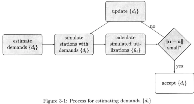
3.5 Simulator details: inferring demands di . . . .
3.6 Validation . . . . 3.6.1 Expert-identified trends . . . . 3.6.2 Reproducing historically observed data . . . .
3.6.3 Stable demands . . . . 17 . . . . 17 . . . . 18 . . . . 26 . . . . 30 . . . . 31 . . . . 40 . . . . 44 47 . . . . 48 . . . . 50 . . . . 52 . . . . 53 . . . . 54 . . . . 57 . . . . 61 . . . . 62 . . . . 63 . . . . 64
4 Case studies
4.1 Boston Case Study . . . . 4.1.1 Choosing weights w . . . .
4.1.2 Inferred demands . . . . 4.2 Manhattan Case Study . . . . 4.3 Conclusion . . . .
5 Search data
5.1 Introduction . . . .
5.2 Search data ... ...
5.3 Search data and data fusion in the literature
5.3.1 Search data . . . .
5.3.2 Data fusion . . . . 5.4 Proposed method . . . . 5.4.1 Discussion . . . . 5.4.2 Remixing strengths and weaknesses .
5.5 Validation . . . . 5.5.1 Density estimation . . . .
5.5.2 Learning weights . . . .
5.5.3 Dependency graph . . . .
5.6 Boston case study . . . .
5.6.1 Remixing structure . . . .
5.6.2 Study region . . . .
5.6.3 Results . . . . 5.6.4 Mixing reservation and search data .
5.7 Conclusion . . . . 6 Conclusion
A Wasserstein distances
B Additional Validation Results
67 68 68 70 73 77 79 79 80 84 84 87 89 92 95 96 96 106 108 113 113 114 115 119 121 123 127 131
C Multivariate Normal Validation Details 135 C.1 Inspiration ... ... 135 C.2 Implementation challenges for MLE . . . . 136 D Grid Search for Reservation Duration Coefficient a 139
List of Figures
2-1 Wasserstein errors of the resampling and MLE methods when D is
exponentially distributed . . . . 36
2-2 Wasserstein errors of the resampling and MLE methods when D is a W eibull distribution . . . . 36
2-3 Wasserstein errors of the resampling and MLE methods when D is norm ally distributed . . . . 37
2-4 Wasserstein errors of the resampling and MLE methods when D is log-normally distributed . . . . 37
2-5 Case study inspired experiment results. The solid line represents er-rors of the MLE method, and the dotted line represents erer-rors of the resam pling method. . . . . 43
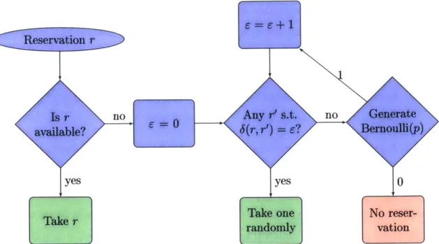
3-1 Process for estimating demands
{di}
. . . . 493-2 Attempting a reservation r . . . . 55
4-1 Density of di - u . . . ... . . . . 72
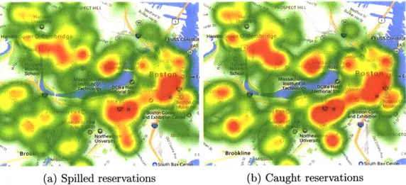
4-2 Density of spilled and caught reservations . . . . 73
4-3 Inferred Manhattan demand, April to June 2017 . . . . 76
5-1 Case study dependency graph . . . . 84
5-2 Wasserstein errors of the remixing and KDE methods for density esti-mation when D is normal or folded-normal . . . . 101
5-3 Wasserstein errors of the remixing and KDE methods for density esti-mation when log(D) is normal or folded normal . . . . 103
5-4 Wasserstein errors of the remixing and KDE methods for density
esti-mation when D is bivariate exponential . . . 105
5-5 Wasserstein distances to D when inferring weights . . . . 109
5-6 Wasserstein distances to D when inferring weights . . . . 110
5-7 Dependency graphs G tested . . . 111
5-8 Search features for tested dependency graphs . . . . 112
5-9 Case study dependency graph . . . . 114
List of Tables
2.1 Average Wasserstein errors under distributional misspecification . . . 38 2.2 Lowest errors of the MLE method under location misspecification of 0.05 39
2.3 Lowest errors of the MLE method under location misspecification of 0.1 39 2.4 Lowest errors of the MLE method under location misspecification of 0.2 40 4.1 Summary of station-wise discrepancies between estimated demand di
and average daily served reservation-hours ui in June 2014 . . . . 71 5.1 Summary of estimated Wasserstein distances between simulated and
historical station-wise usage . . . 120
B.1 Wasserstein errors when D is exponentially distributed with location
param eter 0 . . . . 133
B.2 Wasserstein errors when D has a Weibull distribution with location param eter 0 . . . . 133
B.3 Wasserstein errors when D is normally distributed with location pa-ram eter 0 . . . . 133
B.4 Wasserstein errors when D is log-normally distributed with location param eter 0 . . . . 133
B.5 Wasserstein errors when D is exponentially distributed with location param eter 0.1 . . . . 134 B.6 Wasserstein errors when D has a Weibull distribution with location
B.7 Wasserstein errors when D is normally distributed with location
pa-ram eter 0.1 . . . . 134 B.8 Wasserstein errors when D is log-normally distributed with location
Chapter 1
Introduction
Urban populations are growing as the global population expands and moves into cities. Urban mobility systems must therefore serve the basic needs of ever-more peo-ple while contending with ever-greater congestion. Further, the mobility landscape is evolving as alternatives to private car ownership become increasingly prevalent; these include traditional alternatives such as transit, newer modes such as bike-sharing and ride-sharing, and perhaps imminently arriving modes such as on-demand autonomous vehicles. Additionally, urban transportation has historically been very carbon inten-sive, and combating climate change requires mobility systems which create fewer greenhouse gas emissions.
Given these concerns, it is important to design and optimize transportation sys-tems to be as usable, efficient, and emissions-free as possible. Doing so often requires knowledge about demand: information such as where users are located, where users are traveling to, trip mode preferences, and price sensitivity. Demand information is particularly important when designing new services, which should be implemented to serve unmet transportation needs or incentivize users to switch towards more efficient
forms of mobility.
In this thesis, we study urban mobility from the perspective of car-sharing, a
transportation service in which travelers use cars that they do not own; the vehicles are thus shared between users of the car-sharing service. We focus on round-trip station-based car-sharing, which is one of the most common types of car-sharing
worldwide
14].
In round-trip car-sharing, users must return the vehicle they use to the location where they picked up the vehicle; the alternatives are known as one-way service and free-floating service. 'Station-based' means vehicles are available for pickup and dropoff only at predesignated stations, unlike free-floating car-sharing where vehicles can be found or returned anywhere throughout a defined service region. Though car-sharing originated in Europe in the mid-20th century, it has only become widely popular in the last decades, especially in the United States [5,27].In the round-trip car-sharing context, demand is the number of users who would like to reserve a vehicle. More precisely, demand is a function over reservation at-tributes such as location, duration, vehicle class, and price that specifies the expected number of users who would like a reservation matching those attributes. Demand is not-and cannot be-directly observed, and so it must be inferred from available data. Thus, demand can be considered a latent (unobserved) factor which gives rise to observed data.
In Chapter 2, we propose and validate a general simulation-based method for inferring such a latent distribution; our method is designed for and appropriate in the urban mobility context. We then turn to case studies performed in collaboration with Zipcar, the largest car-sharing operator in the United States. Throughout this thesis we rely on data and domain expertise provided by our Zipcar colleagues. In Chapter 3 we present a custom car-sharing simulator which captures the key mechanics of users competing for reservations. Then in Chapter 4 we describe case studies in the Boston and New York areas which combine the methods of Chapters 2 and 3 with Zipcar data to estimate demand for Zipcar services. In Chapter 5 we consider the extension of our method to search data, i.e. information about what car-sharing reservations users search for. Finally, we conclude in Chapter 6 by considering future trends in mobility analytics.
Chapter 2
Detruncation
2.1
Motivation
When making short-term operational decisions or long-term strategic decisions, the operator of a mobility service might like to know the spatio-temporal patterns in demand for their service. Note that throughout this chapter we use car-sharing as an example of a mobility service; we hope this will enhance the reader's intuition in Chapters 3-5. Nonetheless, the techniques presented in this chapter are quite general and can be naturally applied to other mobility services or beyond the transportation field.
For example, a mobility service operator such as a car-sharing operator (CSO) with knowledge of the temporal patterns in demand for car-sharing may be able to efficiently rotate vehicles in or out of the car-sharing fleet to meet periods of high demand such as holidays and weekends. Understanding spatial patterns in demand is especially important for planning network expansion; the CSO may wish to open new stations near areas of underserved demand.
However, a CSO can never directly observe demand. The ways in which users interact with a car-sharing network are fundamentally an interaction between supply and demand. Potential users are bound by capacity constraints-they cannot use a vehicle when no vehicle is available-and, critically, engage in complicated substi-tution behaviors. When a user cannot use the car-sharing network in the desired
manner (time, location, type of vehicle, etc.), they may choose another use of the system and in doing so affect the capacity available to all other potential users. In light of these supply-demand interactions, data on user actions (such as reservation data) should not a priori be taken as a reliable estimate of demand for car-sharing services.
We understand from our colleagues at Zipcar that with the proliferation of con-sumer smartphones and big data technologies, it has become increasingly common for CSOs and other mobility operators to record data on user searches: instances in which a potential user inquires about the availability or cost of mobility resources. In Chapter 5 we investigate the use of such data in a car-sharing setting. While search data may intuitively seem to be a better proxy for user demand than reservation data, it is also an imperfect measure of demand. For example, a potential car-sharing user might learn that their first choice reservation is unavailable and then search for a substitute reservation; it is not clear to what extent this substitute search repre-sents that user's demand. Additionally, the physical constraints of collecting search data often lead to noise or bias. For example, consider the case where a mobile ap-plication user swipes a map showing availability of car-sharing vehicles: is the user interested in vehicles at the new location to which they moved the map, or did they just accidentally brush their smartphone screen?
Since demand cannot be directly observed, it must be inferred from available data. To the extent that car-sharing usage data can be considered a truncated sample of demand, this can be seen as a detruncation problem. In the remainder of this chap-ter, we consider existing detruncation approaches while noting their strengths and challenges in the car-sharing context. We then propose a simulation-based method and test this method via synthetic validation experiments.
2.2
Detruncation in the literature
The problem of inferring a distribution given an imperfect sample from that distri-bution arises in fields ranging from the natural sciences to management science to
transportation. The relevant problem formulations and even the vocabulary used to describe the problems vary tremendously, but here we highlight some common statis-tical nomenclature
[32,
Ch. 3]. A set of observations from an underlying distribution D is considered censored if the observations are constrained to lie in some set R;draws from D which do not lie within R are projected onto R before being observed. For example, this situation arises naturally in medical studies examining patient mor-tality. The observed survival time of each patient is constrained to lie in the interval from zero to the duration of the study, and the actual survival time for patients who survive to the end of the study is not observed. In contrast, a set of observations is said to be truncated if only those draws from D which lie in R are observed, and no projection is done. For example, asking visitors to a website how frequently they visit the website yields a truncated sample from the distribution of how often all people visit the website; individuals who do not visit are not observed. One can also imagine a situation wherein draws from D are not subject to strict censoring or truncation but are instead modified through some process (possibly non-independent and/or proba-bilistic) before being observed. We are not aware of a common term describing this wide variety of possibilities.
In the car-sharing context, all these mechanisms are at play. Suppose that the underlying distribution D describes car-sharing reservations users would like to make, and the observed data are the reservations actually made. There is censoring because a user who wants a reservations the system cannot serve may instead take the most similar available reservation. There is truncation when a user cannot find an accept-able reservation and thus exits the system without leaving a record in the observed data. And there are a variety of subtler processes arising from price incentives, fleet rebalancing, and so forth. For example, if a vehicle is temporarily removed from ser-vice due to a mechanical problem, all reservations for that vehicle during the serser-vice period must be replaced with roughly comparable reservations. For brevity and clar-ity, throughout the rest of this thesis we use the word "truncation" to describe any combination of censoring, truncation, or other pre-observation modification of data.
recov-ering a latent (i.e. unobserved, but giving rise to observed data) distribution subject to known truncation
[52,
Ch. 91. A likelihood function for observed data is written by assuming a parametric form for the latent distribution and the truncation process,and then the maximum likelihood parameters are inferred. This approach is taken for example in the well-known vending machine study [21 where the unobserved arrival rate of customers is estimated by assuming a simple customer choice model along with a Poisson process for the customer arrival process. The popularity of maximum likelihood approaches is well deserved. MLE techniques are usually computationally efficient whether implemented by directly maximizing the log-likelihood or by using the expectation-maximization algorithm (see e.g. [6, Ch. 9j). In some cases, no max-imization procedure is required because the maximum likelihood parameters can be computed in closed form. Further, the maximum likelihood estimator is known to have asymptotically optimal convergence properties (under mild regularity conditions, see e.g. [30, Ch. 9, 161). Additionally, maximum likelihood estimation often performs well in practice. For a recent comparison of MLE to other inference methods, see [201. However, MLE is not without its challenges. For example, the parameters max-imizing the likelihood can correspond to a pathological or physically meaningless solution. Notably, this is a danger when fitting Gaussian mixture models: infinite likelihood can be attained by having one component of the mixture "collapse" towards a zero-variance singularity at a single data point [6, p4341. In addition, this approach is ill-suited to the car-sharing case because the intricate interdependence of customers' decisions makes writing an analytic likelihood impractical. To illustrate one facet of this interdependence, note that in a car-sharing context, it is common for multiple distinct reservations to be mutually exclusive. For example, the reservations "vehicle
i from 2pm-4pm" and "vehicle i from 3pm-5pm" are distinct products for which there
is likely separate demand, but if a customer takes one of these reservations, no other customer can choose the other. This introduces a complicated time and space de-pendency between reservations: the result of a user searching for a given reservation depends not just on whether that particular reservation is available, but also on the availability of all other reservations the user might accept. As a consequence, the
order in which desired reservations arrive matters and thus reservations are not ex-changeable; this significantly complicates writing a likelihood function which captures the reservation dynamics.
Maximum likelihood techniques typically require practitioners to incorporate spe-cialized domain knowledge when assuming the parametric form of the latent distri-bution and truncation procedure. In the case of car-sharing, such knowledge is often not available. In our case study, for example, a plausible parametric form of the distribution of car-sharing demand is not known a priori, and we arc unable to make plausible distributional assumptions.
There has been some work on using nonparametric methods together with maxi-mum likelihood; for example,
[45]
infers a truncated bivariate density by assuming the only interaction effect between the variables is the simple product of those variables, though the author also suggests using a physically motivated interaction term. This technique would be difficult to apply to the car-sharing demand distribution because demand depends on many factors including day of week, time of day, location, dura-tion, and so forth. Therefore the number of potential interaction terms is large, and we don't a priori know plausible forms for these interaction terms.The problem of recovering a truncated distribution also occurs frequently in rev-enue management where it is often referred to as 'unconstraining': the number of sales of a product is constrained to be less than or equal to the stock of that prod-uct, and a retailer would like to know the unconstrained demand. See [52, Ch. 9 for an overview of common unconstraining methods in revenue management, includ-ing an outline of how the expectation-maximization algorithm is commonly applied to maximum likelihood techniques for unconstraining. For a more recent high-level overview of unconstraining in revenue management, see
[541.
Occasionally, nonpara-metric unconstraining methods are used in revenue management. For example, the classic Kaplan-Meier estimator [291 is a nonparametric estimate of survival probabil-ities given censored survival data. Advantages of the Kaplan-Meier estimator include wide applicability, ease of computation, and ease of interpretation. However, the Kaplan-Meier estimator requires information on when censoring occurred, and thisinformation is not readily available in the car-sharing context. For example, in a rev-enue management context the Kaplan-Meier estimator can be used to estimate total demand; the data required are how many of a product sold each day and whether the sales were right-censored on each day because sales equaled available stock. However, in car-sharing, there are combinatorially many partially substitutable reservations, and it's not a priori clear when a particular reservation type is "out of stock" in the sense that no acceptable substitute reservation is available.
The revenue management literature also contains machine learning-based non-parametric techniques for unconstraining. 1181 use sales data from products which did not sell out to construct nonparametric curve estimates of the portion of total sales as a function of the time a product has been available, and these curves are used to infer total demand for products which did sell out. In car-sharing, we might consider a reservation sold out if that reservation and all acceptable substitutes are taken. Since substitution preferences are not well known in the car-sharing context, the information on which reservations effectively sold out is not readily available.
Our proposed detruncation procedure provides the following methodological con-tributions. Our method is applicable in cases where the parametric form of the latent distribution is unknown, when the latent distribution may be high-dimensional or have non-real support, and when the available data does not indicate when trunca-tion occurred. Thus our resampling method is appropriate in many contexts beyond car-sharing. We do, however, require knowledge of the truncation procedure, or at least a plausible proxy thereof. This knowledge can be in the form of a simulator; an analytic likelihood is not needed. In addition, our method is highly data-driven: it requires fitting few parameters (e.g., one and two parameters are used in the case studies of Sections 4.1 and 4.2, respectively) and no explanatory models. The prin-ciple disadvantages of our method are that: (i) it requires detailed knowledge of the truncation procedure; (ii) it is most applicable when the latent distribution and trun-cated data have similar support; (iii) for some problems, it is more computationally expensive than other methods, though we note that a single standard laptop has enough computational power to apply our method to the Boston and Manhattan
area case studies (Sections 4.1 and 4.2).
Our method is philosophically and intuitively similar to inverse probability weight-ing [25, 46] (IPW) because, like IPW, our method assigns a weight to each post-truncation observation. IPW is a technique for performing analyses on data sampled non-uniformly from a population; the classic application is the Horvitz-Thompson estimator for population means
[25]
given non-uniform sampling from a population. Frequently, IPW is used to correct for missing data: an analysis is to be performed on data from several subjects, and each subject is either a complete case or has some observations missing. Under IPW, the analysis is limited to complete cases, and each case is weighted by the estimated inverse probability of it being complete; this probability must be modeled using additional information about each case. Classic applications of IPW arise in medical research. For example, some patients in a study may not complete every scheduled office visit, in which case patients with full data could be weighted by the inverse probability of having completed every office visit. In this sense, IPW is commonly compared to imputation as a technique for dealing with missing data. For a recent survey of inverse probability weighting methods, see [461. Recent medical research papers which use inverse probability weighting in-clude f28] and[31
wherein IPW is used respectively to validate an unweighted analysis and to correct for missing data. Despite the similarity of our method to IPW, we note two key differences. First, our method does not require modeling the probability of an observation being observed or a case being complete; instead, weights are esti-mated by solving an optimization problem. Second, the weights in our method are not generally interpretable as inverse probabilities. This is because our method for assigning weights to observations (see Section 2.3) requires solving an optimization problem, and the optimization problem may have several distinct optima. Some of these distinct optimal weight assignments may not correspond to inverse probability weights.1 In fact, our method can be used when defining and modeling probabilities is impractical.'For example, if the truncation procedure acts identically on observations x1 and x2, then our
method can learn the total weight assigned to observations x1 and X2 but not how much of that
Within the car-sharing literature, researchers have approached the problem of understanding demand from several angles. Most often, usage data for an existing car-sharing system are used to calibrate a model of system utilization or user utility, and the distinction between observed demand and unobserved lost demand is not con-sidered. In [50], Stillwater et al. use linear regression to relate monthly hours of usage at each station to explanatory variables such as proximity to public transportation and population density. Here, station utilization is used as a proxy for car-sharing demand. In [34], a similar regression technique is used to inform the location of new car-sharing stations. Stillwater et al. note that using observed utilization as a proxy for demand relies on the strong assumption that the CSO has accurately identified and effectively served all demand for car-sharing services; otherwise the utilization will not accurately represent the demand. However, in practice, these conditions are unlikely to hold. For example, [13] reports that high capacity stations have larger catchment areas (the region from which users may come to the station) than small stations. This could well be because many users cannot find a vehicle at their desired station, and their demand spills over to more distant stations (i.e., a user wants a reservation at one station but ends up making a reservation at another "catching" station); large stations are disproportionately likely to catch spillover demand. This suggests a need for research which investigates the spatial distribution of car-sharing demand while modeling the interaction between available capacity and realized demand.
At least one other study 111] has attempted to address these shortcomings by using a simulation methodology to model car-sharing demand without relying on ob-served usage as a proxy for demand. Here Ciari et al. add car-sharing as a modal option to MATSim, an agent-based transportation simulator [24, Ch. 11; this pro-vides highly granular estimates of the spatial distribution of demand for car-sharing services. Though the initial model does not include car-sharing capacity constraints, Ciari et al. find that the model reproduces empirically observed car-sharing behaviors in Zurich, and a follow-up case study in Berlin [10] improves the model by adding capacity constraints and free-floating car-sharing.
demand for on-demand mobility services. Notably,
[39]
develops a discrete-event simulator for a station-based bike-sharing mobility system in New York City. Time-varying demands for travel between each pair of stations are estimated from data with corrections for factors such as truncation due to lack of available bikes at the start of a trip, broken bikes, and bad weather days. The simulator and demand estimation technique are extended in [26], which introduces gradient-like heuristics for finding strategic assignments of bikes and docks to stations. There, demand for travel between each pair of stations is modeled as a time-varying Poisson process with piecewise-constant rate. The approach of modeling demand as a time-varying Poisson process with rates estimated from data is unlikely to transfer well to the car-sharing setting for two reasons. Firstly, car-sharing stations typically have few vehicles and few reservations per day; thus truncation is common and the amount of historical data is limited. Secondly, in car-sharing there is significant heterogeneity in reservation length; reservations may have durations on the order of hours or weeks. This is in contrast to the bike-sharing case, where bikes are typically ridden from one station to another and reservation duration can be well modeled using travel times.Our work studies the distribution of car-sharing demand using a simpler simu-lation tool than an agent-based simulator such as MATSim. We follow Ciari et al.
(2013) in that we use a stochastic simulation methodology to study the spatial
dis-tribution of car-sharing demand, but we do not use a full transportation simulator. Rather, we simulate a simple customer choice model informed by input from industry stakeholders; as a result, our model requires no input data besides the CSO's histor-ical reservation data. That is, our model does not require data that a CSO might not have access to such as population densities or a calibrated origin-destination ma-trix. Our simulator is designed to allow us to simulate the truncation process by which latent car-sharing demand becomes observed reservations, and by applying the detruncation procedure in Section 2.3, we approximately infer the latent demand distribution. As a result, our methodology somewhat differs in focus from Ciari et al.: rather than modeling granular demand at the agent level, we focus on capturing the key relationships between station capacity, the spatial distribution of demand,
and the spatial distribution of reservations. In particular, our primary contributions in the area of car-sharing are (i) the proposal and validation of a simulation-based method for approximately recovering a truncated latent distribution given truncated data and the truncation procedure; (ii) the formulation of a novel data-driven car-sharing simulator which uses this method to enable the approximate inference of the spatial distribution of car-sharing demand while making few parametric assumptions; (iii) the application of these methods for large-scale case studies in the Boston and New York City (United States) metropolitan areas using high-resolution reservation data from the main U.S. car-sharing operator that show how this model can provide insights of practical use.
2.3
Problem statement and proposed method
We consider the following setting of the general detruncation problem. Data x =
X1,... , x, are generated independently and identically distributed (iid) according to
some distribution D over a metric space (S, 6). Except in synthetic validation ex-periments (see Section 2.4), 79 is unknown. Denote by
f
:U'
1 Sm -+U
S"the truncation function which maps unobserved data x to observed data y = f(x). In practice, f would typically not be known perfectly but would instead be approx-imated by some model
f.
Since the problem of estimatingf
is separate from that of inferring D, we simplify the presentation in this chapter by assumingf
is known. The detruncation problem is then to recover D given observed data y and knowledge of the truncation functionf.
More precisely, a method for solving this detruncation problem should produce an estimate b which is a distribution over S. Ideally, $b is close to D. Of course, defining a notion of closeness between distributions means picking a distance or di-vergence measure on the space of distributions over (S, 6). We use the Wasserstein distances, especially the 1-Wasserstein distance (also known as the earth mover's dis-tance) because this measure of distance between distributions accounts for the metric structure 6 of the underlying metric space (S, 6). See Appendix A for more details on
the Wasserstein distance and how we compute it. The following example of the de-truncation problem setting should provide some intuition about why the Wasserstein distance is an appropriate choice.
In the car-sharing context, each user approaches the car-sharing system with a desired reservation. However, vehicle availability, price incentives, and restrictions on the types of allowed reservations (such as minimum reservation duration) may induce the user to make another reservation or no reservation at all. Thus we could consider:
9 S is the space of all possible reservations and 6 is a notion of dissimilarity between reservations;
9 D is the distribution of all desired reservations;
* x is the finite set of reservations users desire in a given time period;
e f is the truncation function wherein a user searches for their desired reservation
and then chooses which, if any, reservation to make;
* y is the set of reservations users actually make.
In this context, an estimate 5 of D is an estimate of the types of reservations users of the car-sharing system desire. Because car-sharing reservations are partially substi-tutable goods, to the extent that 15 does not perfectly match D, it is advantageous for any set of desired reservations sampled from b to be close (as measured by 6) to an equally sized set of reservations which could plausibly have been drawn from D. For example, if D underestimates the fraction of reservations desired at 84 Massachusetts Avenue, it is better if 5 assigns the extra probability mass to reservations nearby at
1 Amherst Street rather than some far away location such as Logan Airport exactly
because reservations on different parts of MIT's campus are more similar to each other than are reservations at MIT and Logan Airport. To capture this intuition, the measure of dissimilarity used to compare D and 19 should be sensitive to the metric
6, as the Wasserstein distance is. The history of the Wasserstein distance stretches
back centuries; for a recent paper with an excellent motivation of the Wasserstein distance see [44, Sec. 4I.
We define a weight function w : S -+ R>O and let $ be the discrete distribution
with support y and P
[b
= y = W(yi)/, w(yj) for i = 1, ... ,m. We abbreviatethis relationship as b = w(y). Intuitively, we want to pick a weight function w such that when we sample iid from b = w(y) and apply
f
to this sample, we get a resulty
close to observed data y. This is formalized by the following problem:minimize E[W(y,
y)]
(2. 1a)w
subject to P w(y) (2.1b)
(zi, ... , ) rl_ (2.1c)
y
=f
(zi, . ., zO) (2. 1d)w(yi) > 0 for i = 1, ... , m. (2.le)
Here q is a positive integer denoting how many observations to draw iid from P before applying f, the zi are drawn from b, and W is the Wasserstein distance. In this formulation, constraints 2.1b-2.1d link observed data y, estimated latent distribution
P, and simulated resampled-retruncated data
y.
That is, D is a weighted empirical sample of y, as described above. From P we sample z with each zi independent, intuitively representing the simulated unseen data x. Applying f to z yieldsy,
the simulated resampled-retruncated data, which should be close to the observed data y. The objective function 2.1a is the expected distance between observed data y and simulated dataS;
the expectation is over any randomness inherent in the truncation functionf
and is typically approximated by sample averaging.In Problem 2.1, the weights w can be any non-negative function of the observed data y. Since optimizing over all non-negative functions is generally intractable, in practice w is parameterized. The exact parameterization can depend on the space
commonly let w be a n-degree polynomial: minimize subject to E[W(y, y)] D= w(y) (zi, . .. ,Z7) r _ y =f(zi, .. ., z 7)
w(y) =1 aj - (yi)i for i = 1,...,m
j=1 (2.2a) (2.2b) (2.2c) (2.2d) (2.2e) (2.2f) (2.2g) w(y) >0 fori= 1,...,Tm aj E R for = 1, ... , K.
In practice, the last constraint that w(yi) > 0 Vi often means many parameter
values a will be infeasible because they would lead to w(yj) < 0 for at least one i. Often it is convenient to slightly alter the formulation so that almost all parameter values will be feasible. Under the reformulation, negative weights are replaced with zero, and a parameter vector a is feasible if at least one weight is strictly positive. This reformulation expands the set of feasible weights w and thus should also lead to an improved optimal objective function value:
minimize subject to E[W(y,
y)]
D =w(y) Zr) id (Zi, . .z7) max(
y, = f (Zi, . . ., Z77)w(yi) = max (0, 1+ a - (yi)i for i = 1,.. ., m
j=1 / max w(y) > 0 a E R for 1,... , K. (2.3a) (2.3b) (2.3c) (2.3d) (2.3e) (2.3f) (2.3g)
this chapter. The principal assumption of Problem 2.3 is that the weights w are a polynomial function of the observed data. When the weights are assumed to be a low-degree polynomial, the resulting simulation-based optimization problem has few
decision variables and is thus typically tractable.
2.4
Validation experiments
We benchmark our resampling detruncation method by comparison to maximum like-lihood estimation. MLE is a natural benchmark both because of its ubiquity and its theoretical efficiency. Under mild assumptions the MLE is known to be asymptotically optimal and empirically performs well even on small samples. Thus for benchmarks where the necessary assumptions (the parametric form of D is known and both the truncation function
f
and the likelihood can be described analytically) hold, the MLE results can be seen as a bound on how well any detruncation method can perform. That is, in such cases no detruncation method can perform asymptotically better than MLE, and the observed practicality of MLE even with limited data should lead us to believe that even with limited data no detruncation method will meaningfully outperform MLE.It is important to note that comparisons between our resampling detruncation and maximum likelihood necessarily give MLE an advantage: maximum likelihood estimation can only be performed when an analytic likelihood can be written and op-timized, whereas our procedure relies on the weaker assumption that the truncation can be simulated. Additionally, MLE relies on prior knowledge about the parametric form of the latent distribution which may not be available, and our method does not require the practitioner to specify what kind of distribution generated the data. Ex-periments where the benchmark maximum likelihood estimation is done with correct or nearly-correct knowledge of the form of the latent distribution should be seen as giving MLE the benefit of accurate background knowledge, which our method does not use.
We present two groups of validation experiments. Section 2.4.1 contains
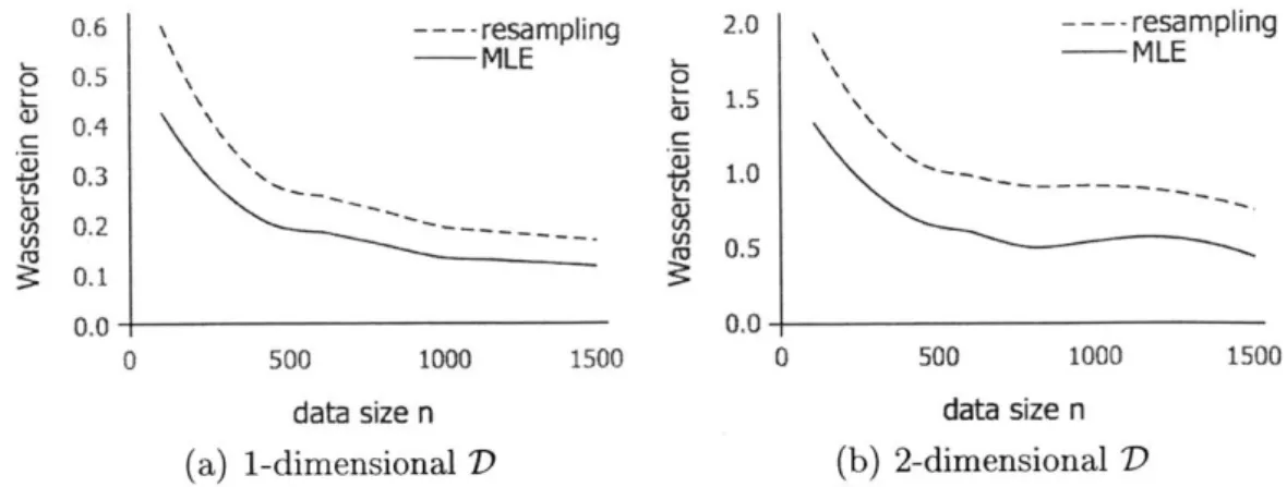
ments where the underlying metric space is the real line, and we vary features such as the latent distribution, the number of data points observed, and the parametric type of the latent distribution used for MLE. This section presents results which suggest that our method is competitive with or even out-performs MLE when the form of the latent distribution is incorrectly guessed. Section 2.4.2 contains a higher dimensional experiment heavily inspired by our car-sharing case studies in Chapter 4.
2.4.1
One dimensional experiments
At a high level, our validation experiments are very simple. First, data x are gener-ated lid from latent distribution D, which is known in these synthetic experiments.
A truncation function
f,
also known perfectly in these experiments, is applied, yield-ing f(x) = y. Given observed data y, we create two estimates of D: bMLEus-ing maximum likelihood estimation and 5 usus-ing our resamplus-ing method. We then compare the Wasserstein distances W(DMLE, D) and W(D, D) to measure how far
each estimate is from the true distribution. The Wasserstein distances W(-, D) are themselves random variables due to randomness in x,
f,
y, and resampled dataz ~w(y). Therefore, for D' E {MLE, b} we estimate E[W(D', D)] by sample
averag-ing: 1W(D', D) =
Z
Ek W(D', D)i where each W(D', D)i is an independent (separate
data x and y, separate inference) realization of W(D', D). In our experiments, we let
k = 5.
The above specification still allows significant freedom in choosing the latent dis-tribution, how many data points x there are, whether the maximum likelihood es-timation problem is correctly specified, and so forth. We allow these experimental parameters to vary independently; that is, we perform an experiment for each unique combination of experimental parameters described below. Each of these elements is now described in more detail.
* Latent distribution We let the latent distribution D be a common continuous
univariate distribution. In particular we consider the exponential distribution with scale 2, the normal distribution with unit variance, the Weibull distribution
with shape 3 and unit scale, and the log-normal distribution where the under-lying normal has expectation 1 and standard deviation 2. These distributions include a variety of qualitative shapes while also having cumulative distribution functions which can be easily differentiated, allowing for efficient MLE infer-ence. We include a location parameter in each distribution's parameterization, including those distributions (such as the exponential distribution) normally parameterized without a location parameter. In these cases, we use the stan-dard trick F(x) = F(x - 1) where F is the standard location-parameter-free
cumulative distribution function, and F is the cdf with location parameter 1. For each distribution, we consider location parameters in {0, 0.05, 0.1, 0.2}.
" Data size We define the data size n as n = jxj, i.e., the number of
pre-truncation data points. We consider n E {10, 20, . . . , 100, 150, 200, ... , 2000}.
" Truncation function We consider a single truncation function
f
which first partitions elements of x into sets of size two uniformly at random and then keeps the minimum element of each set while truncating the maximum element of each pair. Since the x are assumed to be iid, we can write this as yj =min(X2i- 1, x2i), i = 1, ... , n/2.
* Maximum likelihood estimation For each type of distribution (exponen-tial, normal, Weibull, log-normal) that may have given rise to the pre-truncation data, we perform a separate MLE inference. Since in these synthetic experi-ments we know the true latent distribution, we can examine cases where the MLE inference is correctly or incorrectly specified. Additionally, the MLE in-ference is always done assuming a location parameter of 0; maximum likelihood is used to infer only the scale and, as appropriate, shape parameters. Since we consider location parameters {0, 0.05, 0.1, 0.2} for each type of latent distribu-tion, this allows us to examine cases where the MLE inference is not perfectly specified even if the correct type of distribution has been chosen.
op-timization problem (Problem 2.3) using k = 2, i.e., the weight w(y) of an observation y is a quadratic polynomial in y. We approximately solve this two-dimensional problem using a grid search with resolution 0.1 over the region [-.5, 4] x [-.5,4]. Empirically we find that increasing the resolution of the grid search has little effect on final solution quality. While we do not generally rec-ommend brute force methods such as grid search, we use grid search in these validation experiments to allay any concerns that the algorithm used to solve Problem 2.3 does not find a high quality solution.
All together, we consider four families of latent distributions with four location
pa-rameter values each, for a total of 16 latent distributions. We consider 48 different data sizes and four assumed distribution families for MLE inference. So the total number of ILE inferences performed is 5 x 16 x 48 x 4 = 15360, and the total
num-ber of resampling inferences performed is 5 x 16 x 48 = 3840. The complete results from these thousands of experiments are too numerous to detail here, but we include some important and representative results below.
Figures 2-1 through 2-4 summarize results from cases where the maximum like-lihood estimation is performed assuming the correct distributional form of D. Each of these figures has four sub-plots corresponding to the four location parameters we consider. In each subplot, the number of pre-truncation data points n is along the horizontal axis and estimated Wasserstein errors W(D, D') for an inferred distribu-tion D' (either f for resampling or DMLE) are on the vertical axis. For each value of
n we perform 5 trials, where each trial is an independent process of generating data x and y and estimating D, DMLE; the plots show the 5-trial averages. In all the figures, dotted lines represent our resampling approach, and solid lines represent maximum likelihood.
For example, Figure 2-1a in the upper-left of Figure 2-1 corresponds to D an ex-ponential distribution with location parameter 0 and maximum likelihood inference performed assuming that D is an exponential distribution with location parameter
0, i.e., correctly specified. Subfigures 2-1b - 2-1d display the results for experiments
Figure 2-1 shows that errors of both the MLE and resampling methods decrease at similar rates as the number of data points n increases. Perfectly specified MLE asymptotically approaches 0 error, while the error'of the resampling method plateaus higher. However, when D has a nonzero location parameter, the errors of the MLE method are higher than when D has a location parameter of zero because by con-struction the MLE always assumes a location parameter of zero. When the location parameter is 0.1, MLE and resampling are competitive, and when the location pa-rameter is 0.2 (bottom-right subplot), we see that the resampling approach has better performance than MLE except for very small data sizes.
Figure 2-2 is organized the same way as Figure 2-1 but shows results for when D is a Weibull distribution. For all four location parameters considered, the errors of the MLE method are lower than the errors of the resampling method; in each case,
by n = 500 the errors of the resampling method have plateaued to approximately .08
and the errors of the MLE method have plateaued to approximately .02. Here, we see that the MLE performance does not meaningfully change as the location parameter varies. The Weibull distribution has two parameters, shape and scale, and by varying these jointly, MLE can find a location-zero Weibull which closely matches D, even when D has a small but positive location parameter.
Figure 2-3 shows results for when D is a normal distribution. For all four location parameters, after about 250 data points the errors of the resampling method level off around 0.17, and for all four location parameters, after about 500 data points the errors of the MLE method level off around the location parameter. E.g. when the location parameter is 0.1 (and the MLE is still done with a location parameter of 0), the errors of the MLE method approach 0.1. Therefore we see that the MLE performs better than resampling for location parameters in
{0,
0.05, 0.1} and worsefor a location parameter of 0.2.
Figure 2-4 shows results for when D is a log-normal distribution. As with the normal distribution, for location parameters in {0, 0.05, 0.1} the MLE approach beats resampling, and for a location parameter of 0.2 the resampling approach is competitive
therefore the Wasserstein errors (which involve an integral over the whole real line) are higher for a log-normal distribution D than the other considered distributions. We also note one feature of interest: for very small n, occasionally (e.g. consider n = 30 for location parameter 0) inherent randomness in the data leads the maximum likelihood inference to learn a scale normal distribution quite far from the true log-scale normal distribution. Errors in the inferred log-log-scale distribution are magnified through exponentiation, so this leads to quite large errors of the MLE method. For example, consider Figure 2-4a, which shows results from a perfectly specified MLE procedure. At n = 30 there is a spike in the errors of the MLE method arising from one very poor MLE inference. Empirically, this problem is less severe with the resampling method; observe that in each subplot of Figure 2-4, the average error of the resampling method is lower than the average error of the MLE method for some n - [0, 50].
In the experiments summarized in Figures 2-1-2-4, the errors of the resampling method tend not to fall beyond some threshold-for example, around 0.2 when D
is an exponential distribution (Figure 2-1) and 1.7 when D is a normal distribution (Figure 2-3). This is because the weights used for resampling are here constrained to be a quadratic function of the observed data, and the optimal weighting scheme is nonlinear and non-quadratic. In cases with abundant data, the errors of the resam-pling method can be further reduced by considering a larger set of weighting schemes, though this comes at some computational cost. Specifically, finding optimal weights
by solving Problem 2.3 becomes more challenging as the number of decision variables
in Problem 2.3 increases.
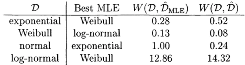
We now consider two cases where the MLE inference is imperfectly specified. First, we consider cases where the maximum likelihood inference is performed under distributional misspecification. That is, for a given latent distribution D, we per-form maximum likelihood inference for each of the distributional types we consider (exponential, Weibull, normal, log-normal) except the type that actually matches D, and we report the best-performing of these misspecified estimates. For example, if
1.5 ---- resampling MLE 1.0 0.5 0.0 0 500 1000 1500 2000 L. . data size n
(a) Location parameter 0.0
1.00 - ---resampling _MLE 0.75 0.50 0.25 0.00 0 500 1000 1500 2000 data size n (c) Location parameter 0.1 C (U M) () 1.5 1.0 - - - -resampling MLE L_ 0 1.5 1.0 - - - -resampling MLE 0.5 0.0 0 500 1000 1500 2000 data size n (d) Location parameter 0.2
Figure 2-1: Wasserstein errors of the resampling and MLE methods when D is expo-nentially distributed 0.25 n2_ I - - - -resampling MLE U. 0.15 0.10 0.05 0.00 0 500 1000 1500 2000 data size n
(a) Location parameter 0.0 0.20 ---- resampling I _MLE 0.15 M 0.10 ' ~-0.05 0.00 0 500 1000 1500 2000 L.. 0 Q) Q) En E) 0 data size n (c) Location parameter 0.1 0.25 n) ' ---- resampling MLE 0.15 0.10 , 0.05 0.00 0 500 1000 1500 2000 data size n (b) Location parameter 0.05 0.15 - - - -resampling StMLE 0.10 0.05 0.00 0 500 1000 1500 2000 data size n (d) Location parameter 0.2
Figure 2-2: Wasserstein errors of the resampling and MLE methods when D is a Weibull distribution 0.5 0.0 0 500 1000 1500 2000 data size n (b) Location parameter 0.05 I-0 C L_ 0 C () (n L_ 0 L.. E)
0.6 0.5 - - - -resampling MLE 0.4 0.3 0.1 0.0 0 500 1000 1500 2000 L. 0 Q.. a) 0.6 0.5 ---- resampling MLE 0.4 0.3 ' 0.2 0.1 0.0 0 500 1000 1500 2000 data size n
(a) Location parameter 0.0 ---- resampling MLE C .a-U) 1... a) 0 500 1000 1500 2000 data size n (c) Location parameter 0.1 data size n (b) Location parameter 0.05 0.6 0.5 0.4 - - - -resampling MLE 0.3 0.2 0.1 0.0 0 500 1000 1500 2000 data size n (d) Location parameter 0.2
Figure 2-3: Wasserstein errors of the resampling and MLE methods when D is nor-mally distributed 40 - - - -resampling MLE 20 10 0 0 500 1000 1500 L_ 0 Z A.-U) L) CU 2000 data size n
(a) Location parameter 0.0
30 - - - -resampling MLE 20 10 -0 0 500 1000 1500 2000 data size n (c) Location parameter 0.1 0 C: 40 - - - -resampling MLE 30 20 10" *-0 0 500 1000 1500 2000 data size n (b) Location parameter 0.05 20 15 10 5 0 --- -resampling MLE 0 500 1000 1500 2000 data size n (d) Location parameter 0.2
Figure 2-4: Wasserstein errors of the resampling and MLE methods when D is log-normally distributed I-0 . L.. 0 1~ L. a) U) 1~ a) U) U) Cu 0.8 0.6 0.4 0.2 0.0 L_ 0 S... 0 Z.. a) i , ', 1
D Best MLE W(D, DMLE) W(D, D)
exponential Weibull 0.28 0.52
Weibull log-normal 0.13 0.08
normal exponential 1.00 0.24
log-normal Weibull 12.86 14.32
Table 2.1: Average Wasserstein errors under distributional misspecification
estimate assuming that D is Weibull, normal, or log-normal. In all these trials, we let n = 100 and set location parameters to 0, which matches the maximum likelihood assumption. Table 2.1 summarizes these results. Each row of the table corresponds to a given D. The columns respectively indicate the parametric form of D, the best performing (among the misspecified) MLE inference, the average error of the MLE method, and the average error of the resampling method. For example, when D is Weibull, the best-performing non-Weibull maximum likelihood estimator is the log-normal estimator with a Wasserstein loss of W(D, DMLE) = 0.13. Overall, Table 2.1 shows that the Wasserstein errors W(D, -) of maximum likelihood with distributional misspecification may slightly larger or smaller than the corresponding errors of the re-sampling method. The case of when D is an exponential distribution (first row of the table) is particularly interesting: the Weibull distribution generalizes the exponential distribution, so maximum likelihood inference assuming a Weibull distribution should be able to exactly recover D when D is an exponential distribution. But with only 100 raw (i.e., 50 observed) data points, the flexibility provided by the shape parameter of the Weibull distribution (which should be exactly 1 for the Weibull to reduce to an exponential) allows over-fitting, and the errors of the MLE and resampling methods have similar orders of magnitude.
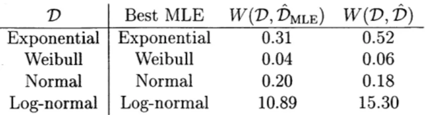
We also consider parametric (rather than distributional) misspecification by giv-ing D a nonzero location parameter; recall that the MLE inference assumes a location parameter of zero. In this case, we report the best MLE estimate, which may be from assuming the correct distribution type or another type. We again consider those trials with n = 100 and location parameters of 0.05, 0.1, and 0.2. These results are