UNIVERSITÉ DE MONTRÉAL
A LOCATION ROUTING PROTOCOL BASED ON SMART ANTENNAS FOR
WIRELESS SENSOR NETWORKS
NELLY POLO
DÉPARTEMENT DE GÉNIE INFORMATIQUE ET GÉNIE LOGICIEL ÉCOLE POLYTECHNIQUE DE MONTRÉAL
MÉMOIRE PRÉSENTÉ EN VUE DE L’OBTENTION DU DIPLÔME DE MAÎTRISE ÈS SCIENCES APPLIQUÉES
(GÉNIE INFORMATIQUE) JUIN 2010
UNIVERSITÉ DE MONTRÉAL
ÉCOLE POLYTECHNIQUE DE MONTRÉAL
Ce mémoire intitulé:
A LOCATION ROUTING PROTOCOL BASED ON SMART ANTENNAS FOR WIRELESS SENSOR NETWORKS
présenté par : POLO Nelly
en vue de l’obtention du diplôme de : Maîtrise ès sciences appliquées a été dûment accepté par le jury d’examen constitué de :
Mme BOUCHENEB Hanifa, Doctorat, présidente
M.QUINTERO Alejandro, Doct, membre et directeur de recherche M.PIERRE Samuel, Ph.D., membre et codirecteur de recherche Mme NICOLESCU Gabriela, Doct, membre
ACKNOWLEDGEMENTS
First of all I would like to thank God, who guides me in my everyday life and activities.
I would like to thank my director of research, Mr. Alejandro Quintero for his support, patience, encouragement and good advice. Also, I would like to thank Mr. Samuel Pierre, my co-director or research, for welcoming me into LARIM (Laboratoire de recherche en réseautique et informatique mobile) and for his availability.
I owe my deepest gratitude to me fellow colleague and friend Luis Cobo for all his support, help, encouragement and advice, without whom none of this would have been possible.
I would like to thank my parents, my brother and my sister for their endless love and support. Thanks for not letting me forget who I am.
Thanks to my “other” family, Diane and Michäel for their patience, support and encouragement. Finally, I would like to thank all my friends, especially Sandra, Arthur and Sergio for all their support, patience, company and encouragement. Thanks for not letting me give up.
RÉSUMÉ
Les réseaux de capteurs sans fil sont une technologie émergente pour la surveillance de l’environnement. Un réseau de capteurs typique se compose d'un grand nombre de capteurs miniatures (nœuds) multifonctionnels, à faible coût et à faible consommation d’énergie, équipés d’un radio émetteur-récepteur et d’un ensemble de transducteurs pour récolter et transmettre des données environnementales d'une manière autonome.
Une des contraintes les plus importantes de capteurs est la nécessitée d’économiser de l’énergie puisqu’ils utilisent des batteries de duré limitée, généralement irremplaçables. En outre, ils se caractérisent également par une faible vitesse de traitement, capacité de stockage et de bande passante, qui nécessite une gestion des ressources très attentive.
En raison des limitations et caractéristiques inhérentes aux capteurs, le routage dans les réseaux de capteurs sans fil suppose un vrai défi. La tâche de trouver et de maintenir des routes n'est pas triviale étant donné les restrictions d'énergie et les changements soudains dans l'état des nœuds (exemple: mal-fonctionnement) qui entrainent des changements fréquents et imprévisibles dans la structure topologique.
Ce travail présente LBRA, un nouveau protocole de routage géolocalisé qui utilise des antennes intelligentes pour estimer les positions des nœuds dans le réseau, et qui base les décisions de routage sur l’état de connexion des voisins et leur position relative.
L'objectif principal de LBRA est d'éliminer le trafic de contrôle du réseau autant que possible. Pour atteindre cet objectif, l'algorithme emploie la position locale pour prendre des décisions de routage, met en œuvre un nouveau mécanisme pour recueillir les informations de localisation et utilise seulement les nœuds impliqués dans la route pour faire la synchronisation des données de positionnement. De plus, le protocole considère le niveau de la batterie au moment de prendre des décisions de routage afin de balancer la dépense d’énergie du réseau.
LBRA est une version améliorée du routage de ZigBee (norme actuelle pour les réseaux à faible coût et à faible consommation d’énergie) qui se base, lui aussi, sur AODV.
Afin d'évaluer dans quelle mesure LBRA représente vraiment une amélioration par rapport au routage de ZigBee, une série de simulations a été effectué à l'aide du logiciel Network Simulator (ns). Les deux protocoles ont été implantés dans le simulateur. Les performances ont été
comparées dans une variété de scenarios, dans des conditions différentes tels que les charges de trafic, les tailles de réseau et les conditions de mobilité.
Les résultats des expériences ont montré que LBRA réussi à réduire le trafic de contrôle et la charge de routage, tout en améliorant le taux de livraison des paquets, à la fois pour les réseaux fixes et les réseaux mobiles. L'abaissement de l'alimentation du réseau est aussi plus équilibré, puisque les décisions de routage sont prises en fonction du niveau de la batterie des nœuds.
ABSTRACT
Wireless sensor networks are an emerging technology for environmental monitoring. A typical sensor network is composed of a large number of low-cost, low-power, multi-functional miniature sensor devices (nodes) equipped with a radio transceiver and a set of transducers utilized to acquire information about the surrounding environment.
One of the most important constraints of sensor nodes is the low power consumption requirement since they carry limited, generally irreplaceable, batteries. In addition, they are also characterized by scarce processing speed, storage capacity and communication bandwidth, thus requiring careful resource management.
Due to the inherent characteristics and restrictions of sensor nodes, routing in WSNs is very challenging. The task of finding and maintaining routes is nontrivial since energy restrictions and sudden changes in node status (e.g. failure) cause frequent and unpredictable topological changes.
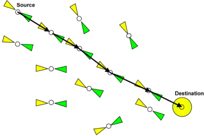
This work introduces a novel location routing protocol that uses smart antennas to estimate nodes positions into the network and to deliver information basing routing decisions on neighbour’s status connection and relative position, named LBRA.
The main purpose of LBRA is to eliminate network control overhead as much as possible. To achieve this goal, the algorithm employs local position for route decision, implements a novel mechanism to collect the location information and involves only route participants in the synchronization of location information. In addition, the protocol uses node battery information to make power aware routing decisions.
LBRA is an enhanced version of the ZigBee routing, which is the current standard for reliable, cost-effective and low power wireless networking, and like the latter is prototyped from AODV. In order to asses to what extent LBRA truly represents an improvement with respect to the ZigBee routing, a series of simulations were designed with the help of the Network Simulator
(ns). Basically, both protocols were implemented in the simulator and its performance was
compared in a variety of traffic load, network size and mobility conditions.
The experiment results showed that LBRA succeed in reducing the control overhead and the routing load, improving the packet delivery rate for both static and mobile networks. Additionally, network power depletion is more balanced, since routing decisions are made depending on nodes’ battery level.
CONDENSÉ EN FRANÇAIS
Les réseaux de capteurs sans fil sont une technologie émergente à faible coût pour la surveillance non-gardée d'un large éventail d'environnements. Ces types de réseaux devrait avoir un impact majeur dans multiple domaines telles que la surveillance, des diagnostics médicaux, le suivi d'objets, surveillance de l'environnement, etc.
Un réseau de capteurs sans fil (RCSF) typique se compose d'un grand nombre de capteurs miniatures (nœuds) multifonctionnels, à faible coût et à faible consommation d’énergie, équipés d’un radio émetteur-récepteur et d’un ensemble de transducteurs pour récolter et transmettre des données environnementales d'une manière autonome.
Un nœud capteur comporte quatre composantes principales: une unité de détection, une unité de traitement, un émetteur-récepteur et une unité d’énergie. Selon l'application et l'objectif spécifique du réseau, le capteur peut nécessiter d'autres composantes telles qu’un système de localisation, un générateur d’énergie, et un dispositif pour le faire bouger. Ces capteurs densément dispersés à l'intérieur d'un phénomène ou très près de lui, ont la capacité de détecter et de réagir aux événements qui se produisent dans leur voisinage [1-3].
Lorsqu'ils sont déployés en grande quantité et en réseau dans un environnement sans fil, ces capteurs peuvent automatiquement s'organiser en réseau ad hoc pour communiquer les uns avec les autres et avec un ou plusieurs nœud-puits (point de collecte) afin de fournir un résultat global de leur fonctionnalité de détection.
Applications des réseaux de capteurs sans fil
Les réseaux de capteurs peuvent être constitués de nombreux types de capteurs tels que sismique, de faible taux d'échantillonnage magnétique, thermique, visuel, infrarouge, acoustique, et les radars, qui sont en mesure de contrôler un large assortiment de conditions ambiantes. Les domaines d’application de cette technologie sont multiples. Par exemple [2] :
– Surveillance des forces, de l'équipement et des munitions – Surveillance des champs de bataille
• L’environnement
– Détection des feux de forêt – Détection d’inondations [12] • Le domaine de la santé
– Administration de médicaments dans les hôpitaux – Télésurveillance de données physiologiques [13] • Le domaine résidentiel
– Domotique [15]
– Environnement intelligent [16] • Le domaine commercial
– Musées interactifs [17]
– Détection et suivi de vols de voitures [18]
– Contrôle environnemental des immeubles à bureaux [17]
Une des contraintes les plus importantes de capteurs est la nécessitée d’économiser de l’énergie puisqu’ils utilisent des batteries de duré limitée, généralement irremplaçables. En outre, ils se caractérisent également par une faible vitesse de traitement, capacité de stockage et de bande passante, qui nécessite une gestion des ressources très attentive. En raison des limitations et caractéristiques inhérentes aux capteurs, le routage dans les réseaux de capteurs sans fil suppose un vrai défi. La tâche de trouver et de maintenir des routes n'est pas triviale étant donné les restrictions d'énergie et les changements soudains dans l'état des nœuds (exemple: mal-fonctionnement) qui entrainent des changements fréquents et imprévisibles dans la structure topologique.
Ce travail présente LBRA, un nouveau protocole de routage géolocalisé qui utilise des antennes intelligentes pour estimer les positions des nœuds dans le réseau, et qui base ses décisions de routage sur l’état de connexion des voisins et leur position relative.
Définitions et concepts de base
En plus des caractéristiques particulières des capteurs tels que les sources d'énergie irremplaçables et des limitations en vitesse de traitement, capacité de stockage et de bande passante, d'autres facteurs affectent aussi le processus de routage. Parmi eux, on trouve [1,3,4]:
1. La consommation d’énergie : extrêmement importante, car la durée de capteur dépend fortement de la durée de batterie, ce qui rend critique le développement de formes de communication qui assurent des économies d’énergie.
2. Déploiement des Nœuds : peut être manuel (où les nœuds sont placés un par un) ou aléatoire (où les nœuds sont jetés en masse) en fonction de la demande.
3. La tolérance de panne : puisque les nœuds sont sujets à mal fonctionner et ces pannes ne devraient pas affecter la tâche globale du réseau de capteurs.
4. Modèle de gestion des données : fait référence à la façon dont les données son livrées aux puits. Ce modèle dépend de l’application et a un impact majeur sur le processus de routage (particulièrement en ce qui concerne l'utilisation optimale de l'énergie et la stabilité des routes), car il détermine le flux de données.
5. Agrégation des données : qui est la combinaison de données provenant de différentes sources pour en quelque sorte alléger la redondance.
6. Extensibilité : puisque le nombre de nœuds déployés dans la zone de détection peut être de l'ordre de centaines, de milliers, ou plus, et des algorithmes de routage doivent être en mesure de faire face à cette situation.
Le routage dans les réseaux de capteurs se classe généralement en : « centré sur les
données », « hiérarchique » ou « basé sur la localisation ». En plus, selon la façon dont
la source trouve la destination, les protocoles de routage peuvent être classés en « proactive » dans laquelle les routes sont établies à l’avance, « réactive » dans laquelle les routes sont établies à la demande ou « hybride » qui combine les deux autres.
Dans le routage centré sur les données, le puits envoie des requêtes à certaines régions et attend les données provenant de capteurs situés dans ces régions. Dans ce genre de réseaux chaque nœud joue généralement le même rôle et les capteurs collaborent pour accomplir la tâche de détection.
Dans le routage hiérarchique, s’effectue une division du réseau en plusieurs sous-ensembles ou régions. L’objectif principal de ce type de routage est de maintenir efficacement la consommation d’énergie par l’agrégation des données afin de diminuer le nombre des messages transmis. Dans chacune de ces régions la transmission de paquets est effectuée par le biais d'un système de coordonnées locales et la communication entre les régions est effectuée pour diriger les données vers le nœud-puits. Dans cette approche les nœuds jouent des rôles différents dans le réseau.
Dans le routage basé sur la localisation, la position des capteurs est exploitée pour acheminer les données dans le réseau. Chaque nœud décide à quel voisin transmettre le message basé uniquement sur son emplacement, celui de ces voisins, et celui de la destination [5]. L’information de la localisation est principalement utilisée pour calculer la distance entre deux nœuds afin d’estimer la consommation d'énergie nécessaire pour la communication.
Aspects du problème
Le routage dans les réseaux de capteurs sans fil est très difficile en raison des caractéristiques particulières qu’ils possèdent et qui les distinguent des réseaux de communication traditionnelles et des réseaux ad hoc. Ces distinctions font que l’utilisation des mécanismes de routage spécialement conçus pour ces types de réseaux n’est pas appropriée. Les principales différences sont [1-4]:
1. Il n'est pas possible de construire un système d'adressage global pour le déploiement d'un grand nombre de capteurs puisque la charge d'entretien des identificateurs est élevée.
En plus, les protocoles de routage basés sur IP traditionnels font le routage en utilisant l'adresse de destination et l’information stockée dans les tables de routage qui indique
le prochain saut vers cette destination. Cependant, dans les réseaux de capteurs sans fil, où les nœuds peuvent être déployés de manière aléatoire et en grande quantité, et qui ont des variations de topologie fréquentes dues aux pannes ou aux changement dans l’état des nœuds pour économiser de l’énergie, la surcharge des messages nécessaires pour maintenir les tables de routage et l'espace de mémoire requis pour les stocker n'est pas abordable [3].
Par conséquent, les protocoles classiques basés sur IP ne peuvent pas être appliqués aux RCSFs.
2. La plupart des applications de réseaux de capteurs requiert le flux des données captées à partir de sources multiples pour un récepteur unique.
3. Les données générées sont très redondantes étant donné que plusieurs capteurs situés dans la même région peuvent générer des données identiques. Cette redondance doit être exploitée par les protocoles de routage afin d’améliorer l'efficacité énergétique et l'utilisation de bande passante.
4. Les capteurs sont fortement limités en termes de ressources, ce qui nécessite une gestion minutieuse.
5. Les réseaux de capteurs sont spécifiques à l'application (c'est-à-dire : la conception d'un réseau de capteurs dépend de l’application).
Bien que de nombreux algorithmes de routage pour les RCSF aient été proposés à la suite des différentes approches qui existent, dans [6] il a été démontré que les protocoles de routage qui n'utilisent pas des informations de localisation géographique ne sont pas extensibles. En plus, dans [3] il a été établi que les protocoles de routage idéaux pour le RCSF doivent baser les décisions de routage sur les informations échangées entre les nœuds voisins, offrir la fiabilité dans le réseau, et requérir un minimum de trafic de control, consommation d'énergie et encombrement de mémoire. Pour ces raisons, la plupart des recherches sur le routage dans les RCSF sont concentrées sur les protocoles géolocalisés ou basées sur la localisation.
Les algorithmes de routage géolocalisés évitent la surcharge de trafic de contrôle en limitant l’échange de messages au minimum pour connaître la position exacte des voisins et avoir une idée approximative de la position de la destination. Ceci est très pratique pour les réseaux avec des contraintes d’énergie critiques comme les RCSF [5]. En outre, des informations de localisation peuvent également être utilisées pour identifier une source de données selon les besoins de l'application. Nonobstant, l'utilisation de protocoles géolocalisés pose aussi des problèmes évidents en termes de fiabilité. La précision de la position de la destination est un problème important à considérer.
La méthode la plus simple pour résoudre le problème de localisation est d’équiper tous les nœuds d'un récepteur GPS qui permettrait d'assigner des coordonnées réelles aux nœuds dans le réseau. Toutefois, cette solution est coûteuse en raison des coûts du récepteur GPS, la consommation d'énergie et les exigences de format. De plus, la méthode peut échouer si tous les nœuds ne reçoivent pas les signaux GPS.
Une bonne alternative serait d’équiper d’un récepteur GPS (ou fournir manuellement des coordonnées correctes) seulement quelques nœuds, et sur cette base, calculer les coordonnées d'autres nœuds. Néanmoins, bien que cette solution soit moins onéreuse que la première en termes de nombre total de récepteurs GPS nécessaires, elle pourrait être plus coûteuse en termes de trafic de contrôle et de consommation d'énergie, dû à l'échange d'informations nécessaires pour calculer les coordonnées d’autres nœuds. Il pourrait aussi y avoir des erreurs importantes de mesure et d'approximation.
Une autre solution consiste à assigner des coordonnées virtuelles aux nœuds en fonction de la connectivité du réseau; les coordonnées relatives des nœuds voisins sont obtenues en échangeant ces informations entre voisins.
Le principal inconvénient de cette solution est que cela entraîne une complexité importante des calculs et une surcharge des messages (inondations). De plus, elle requiert un espace de mémoire dans le nœud, déjà fortement limitée.
Une nouvelle approche, qui est restée inexplorée jusqu'à tout récemment, est l'utilisation d'antennes intelligentes. Elles permettent l’estimation précise des positions des nœuds,
améliorent la communication dans le réseau en diminuant la consommation d'énergie et, par conséquent, augmentent sa durée de vie.
Une antenne intelligente est une antenne composée de nombreux éléments d'antenne qui sont disposées de façon linéaire, circulaire ou planar. Leur rôle est d'augmenter la qualité du signal radio par l'optimisation de la propagation radioélectrique et accroître la capacité du medium en augmentant l'utilisation de bande passante. Leur intelligence réside dans la combinaison des signaux reçus dans les éléments d'antennes intelligentes [7].
Les antennes intelligentes ont été longtemps considérées comme inappropriées pour les RCSF à cause de leur volume plus grand que les antennes traditionnelles dû au plus grand nombre d’éléments d’antenne. Le traitement de plus d'un signal nécessite, également une plus grande puissance de calcul et une électronique capable de traduire la fréquence radio (RF) en une bande de base appropriés.
Toutefois, il a été démontré expérimentalement que l'utilisation des antennes intelligentes peut augmenter la capacité globale du réseau et réduire considérablement la consommation d'énergie. En outre, il a été démontré que l'utilisation des antennes intelligentes dans les réseaux de capteur est obligatoire dans certains cas, et possible dans d'autres, pour un coût supplémentaire minimal [7-10].
LBRA (The location based routing algorithm)
L'objectif principal de LBRA est d'éliminer le trafic de contrôle du réseau autant que possible. Pour atteindre cet objectif, l'algorithme emploie la position locale pour prendre des décisions de routage, met en œuvre un nouveau mécanisme pour recueillir les informations de localisation et utilise seulement les nœuds impliqués dans la route pour faire la synchronisation des données de positionnement. De plus, le protocole considère le niveau de la batterie au moment de prendre des décisions de routage afin d’équilibrer la dépense d’énergie du réseau.
LBRA est une version améliorée du routage de ZigBee (norme actuelle pour les réseaux à faible coût et à faible consommation d’énergie) qui se base, lui aussi, sur AODV.
1. Découverte de la route (RD), dans lequel les nœuds cherchent des routes pour communiquer entre eux.
2. Établissement de la route (RE), dans lequel les nœuds établissent des connexions dans les deux sens par l’échange des informations requises
3. Maintenance de la route (RM), qui constitue un mécanisme pour sélectionner la meilleure route en termes de consommation d'énergie parmi les routes trouvés pendant la phase de découverte.
La découverte de la route, à son tour est divisée en deux étapes:
1. Route-demande (RREQ), dans lequel un nœud source cherche un nœud destination spécifique dans le réseau.
2. Route-réponse (RREP) qui permet la mise en place de la route de communication bidirectionnelle entre les nœuds, une fois que le nœud de destination est trouvé.
En LBRA il y a deux scénarios possibles pour le processus de RD: l’inondation et l’inondation limitée. Le choix du scénario dépendra de la connaissance de la position du nœud de destination: si le nœud source connaît l'emplacement du nœud de destination, il utilise l’inondation limitée, sinon, il inonde l'ensemble du réseau.
Le processus de découverte de la route se fait soit lorsque le nœud source ne connaît pas de route pour atteindre le nœud de destination, ou si une route préalablement établi entre eux n'est plus disponible. Dans cette dernière situation, puisque les nœuds ont déjà communiqué, les emplacements de chaque nœud est disponible et au lieu d'inonder l'ensemble du réseau à la recherche d'une route, LBRA passera au scénario d’inondation limitée en la restreignant à une zone spécifique, appelé la zone cible.
En LBRA, en plus d’établir des connexions entre les nœuds, les inondations servent également à synchroniser les informations de localisation dans le réseau et à calculer le coût de relai, qui correspond à la somme du coût d’utilisation des nœuds appartenant à la route qui est explorée.
Lorsqu’un processus de découverte de route est déclenché, le nœud source peut recevoir de nombreux messages de réponse (RREP), chacun avec une route différente vers le nœud
de destination. En général, l'ordre d'arrivée de ces messages ne dépend que du nombre de nœuds qui composent la route: moins il y aura de nœuds dans la route, plus la réponse atteindra la destination rapidement. Toutefois, en termes de consommation d'énergie, la meilleure route ne sera pas nécessairement celle qui a le moins de nœuds.
En LBRA, cette situation est traitée par l'acceptation subséquente de messages de réponse et le remplacement de la route, si le coût de la transmission de la nouvelle est moins élevé. Pourtant, le nœud source commencera la transmission de données dès que la première route sera découverte sans tenir compte qu’elle soit optimale en termes d’énergie ou non.
Afin d'évaluer dans quelle mesure LBRA représente vraiment une amélioration par rapport au routage de ZigBee, une série de simulations a été effectué à l'aide du logiciel Network Simulator (ns). Les deux protocoles ont été implantés dans le simulateur. Les performances ont été comparées dans une variété de scenarios, dans des conditions différentes tels que les charges de trafic, les tailles de réseau et les conditions de mobilité (réseaux mobiles et statiques).
Les expériences ont été réalisées avec les nœuds statiques et en mouvement, avec les nœuds se déplaçant à différentes vitesses et avec des topologies différentes. Pour chacune des expériences, quatre scénarios ont été utilisés, avec plusieurs charges de trafic: faible, moyenne, normale et haute.
Les résultats des expériences ont montré que LBRA réussi à réduire le trafic de contrôle et la charge de routage, tout en améliorant le taux de livraison des paquets, à la fois pour les réseaux fixes et les réseaux mobiles. L'abaissement de l'alimentation du réseau est aussi plus équilibré, puisque les décisions de routage sont prises en fonction du niveau de la batterie des nœuds.
INDEX
ACKNOWLEDGEMENTS ...iii
RÉSUMÉ... iv
ABSTRACT ... vi
CONDENSÉ EN FRANÇAIS ...vii
INDEX ... xvi
INDEX OF TABLES ... xix
INDEX OF FIGURES... xx
LIST OF ACRONYSMS AND ABREVIATIONS ...xxii
CHAPTER 1 INTRODUCTION... 1
1.1 Definitions and basic concepts ... 1
1.2 Aspects of the problem... 2
1.3 Research goals... 5
1.4 Outline... 5
CHAPTER 2 ROUTING IN WIRELESS SENSOR NETWORKS... 6
2.1 Sensor networks applications ... 6
2.2 Types of sensor networks ... 7
2.3 WSNs architecture... 8
2.3.1 Protocol stack ... 8
2.4 Design issues ... 10
2.4.1 Energy consumption... 11
2.4.2 Data management model ... 11
2.4.3 Node deployment ... 12
2.4.4 Data aggregation/fusion ... 12
2.4.5 Scalability... 12
2.4.6 Fault tolerance ... 12
2.5 Routing challenges in WSNs... 13
2.5.1 Data-centric routing... 14
2.5.2 Hierarchical based routing ... 15
2.5.3 Location based routing ... 16
2.6 Sensor networks based on smart antennas ... 20
2.6.1 Definition and overview... 20
2.6.2 Smart antenna systems in sensor networks ... 21
2.7 The ZigBee Standard... 22
2.7.1 Network Formation ... 23
2.7.2 Routing ... 25
CHAPTER 3 PROPOSED LOCATION ROUTING ALGORITHM BASED ON SMART ANTENNAS FOR WIRELESS SENSOR NETWORKS... 30
3.1 WSNs routing protocols performance criteria ... 30
3.2 Location aided Routing in WSNs... 32
3.3 The location based routing algorithm (LBRA) ... 35
3.3.1 Route Discovery ... 36
3.3.2 Route Establishment... 44
3.3.3 Route Maintenance... 45
CHAPTER 4 SIMULATION MODEL AND RESULTS... 48
4.1 Simulation Design ... 48
4.1.1 The network simulator ... 48
4.1.2 Simulation remarks ... 49
4.1.3 Basic configuration ... 50
4.2 Simulation results and analysis ... 50
4.2.1 Performance evaluation... 50
4.3 Impact of network size on the protocol performance... 57
4.4 Impact of nodes mobility on the protocol performance ... 63
4.4.1 Mobility model... 63
4.4.2 Mobility simulation results and analysis ... 64
CHAPTER 5 CONCLUSION ... 72
5.1 Summary of the work ... 72
5.2 Limitations of research... 73
5.3 Future work ... 73
INDEX OF TABLES
Table 2.1: ZigBee routing table... 25
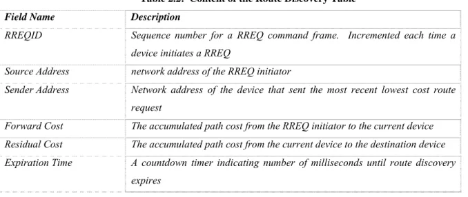
Table 2.2: Content of the Route Discovery Table... 27
Table 3.1: LBRA routing table... 36
INDEX OF FIGURES
Figure 2.1: Sensor network topology ... 8
Figure 2.2: The sensor network protocol Stack... 10
Figure 2.3: Routing tree ... 16
Figure 2.4: Greedy routing ... 17
Figure 2.5: Dead end in greedy routing... 17
Figure 2.6: Example of virtual grid in GAF [36] ... 19
Figure 2.7: State transitions in GAF [4] ... 20
Figure 2.8: Delivery of information using smart antennas... 22
Figure 2.9: Address allocation for Rm = 2, Dm = 2 and Lm = 3 ... 25
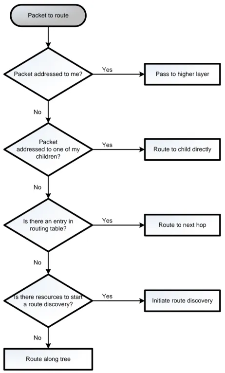
Figure 2.10: Routing protocol ... 26
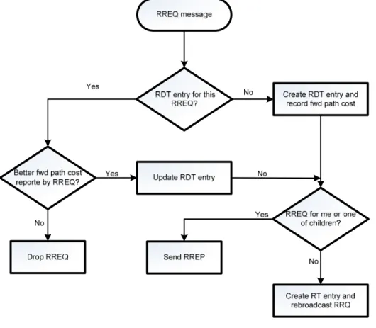
Figure 2.11: RREQ processing... 28
Figure 2.12: RREP processing ... 29
Figure 3.1: Flooding... 37
Figure 3.2: Target zone setup for the limited flooding ... 38
Figure 3.3: Location synchronization... 39
Figure 3.4: LBRA RREQ Process... 43
Figure 3.5: LBRA RREP process... 44
Figure 3.6: Route construction applying RREQ delay... 47
Figure 4.1: Topology 1 with 50 nodes ... 51
Figure 4.2: Average packet delivery rate comparison... 52
Figure 4.3: Average routing overhead comparison ... 54
Figure 4.4: Average control overhead comparison ... 56
Figure 4.5: Topology with 100 nodes ... 58
Figure 4.6: Topology with 200 nodes ... 58
Figure 4.7: Packet delivery rate comparisons for networks with 50, 100 and 200 nodes... 59
Figure 4.8: Control overhead comparisons for networks with 50, 100 and 200 nodes... 60
Figure 4.9: Average routing load comparison for networks with 50, 100 and 200 nodes ... 62
Figure 4.10: Average packet delivery rate comparison for mobile networks ... 64
Figure 4.11: Average control overhead comparison for mobile networks... 66
Figure 4.13: Influence of nodes' speed on the average packet delivery rate... 69 Figure 4.14: Influence of nodes' speed on the average control overhead ... 70 Figure 4.15: Influence of nodes' speed on the average routing load ... 71
LIST OF ACRONYSMS AND ABREVIATIONS
AOA Angel of Arrival
AODV Ad hoc On Demand Distance Vector
CONSER Collaborative Simulation for Education and Research DARPA Defense Advanced Research Projects Agency
DID Destination Node Identifier
DSR Dynamic Source Routing protocol
ESPRIT Estimation of Signal Parameters via Rotational Invariance Techniques GPS Global Positioning System
ICIR ICSI Center for Internet Research ICSI International Computer Science Institute
IP Internet Protocol
LBL Lawrence Berkeley National Laboratory
MAC Medium Access Control
MN Mobile Node
MUSIC Multiple Signal Identification and Classification MVDR Minimum Variance Distortionless Response
NS Network Simulator
NSF National Science Foundation
PAN Personal Area Network
PARC Palo Alto Research Center PHY Physical
QoS Quality of Service
RD Route Discovery
RDT Route Discovery Table
RE Route Establishment
RF Radio Frequency
RM Route Maintenance
RREP Route Reply
RREQID Route Request Identifier
RSSI Received Signal Strength Indicator
RT Routing Table
SAMAN Simulation Augmented by Measurement and Analysis for Networks SID Source Node Identifier
SNR Signal Noise Ratio
Tcl Tool command language
TCP Transmission Control Protocol TDOA Time Difference of Arrival
TOA Time of Arrival
UCB University of California in Berkeley
UDP User Datagram Protocol
USC/ISI The Information science institute of the Universiti of southern California VINT Virtual Inter Network Testbed
WSN Wireless Sensor Network
ZC ZigBee Coordinator
ZED ZigBee End Device
CHAPTER 1
INTRODUCTION
Wireless Sensor Networks (WSNs) are an emerging technology for low cost, unattended monitoring of a wide range of environments. These kinds of networks are expected to have major impact on multiple application scenarios such as surveillance, environmental monitoring, medical diagnosis, object tracking, etc.
A WSN is composed of a sheer number of sensors nodes capable of observing and reacting to changes in ambient conditions in the environment surrounding them and then transforming these measurements into signals that can be processed. When networked together these sensor nodes, fitted up with transceivers to communicate either among each other or directly to an external base station (sink), coordinate among themselves to produce high-quality information about the physical environment. Each sensor node bases its decisions on its mission, the information it currently has and its knowledge of its computing, communication, and energy resources [1-3]. One of the most important constraints of sensor nodes is the low power consumption requirement since they carry limited, generally irreplaceable, batteries. In addition, they are also characterized by scarce processing speed, storage capacity and communication bandwidth, thus requiring careful resource management.
Due to the inherent characteristics and restrictions of sensor nodes, routing in WSNs is very challenging. The task of finding and maintaining routes is nontrivial since energy restrictions and sudden changes in node status (e.g. failure) cause frequent and unpredictable topological changes [1].
This work presents a novel location routing protocol based on smart antennas for wireless sensor networks. This introductory chapter presents the basic concepts of WSNs and the elements of the problem, followed by our research’s objectives and finally the outline.
1.1 Definitions and basic concepts
Besides the special characteristics of sensor nodes such as irreplaceable power sources and limited processing speed, storage capacity and communication bandwidth, other factors also affect the routing process. Among them we found: energy consumption, extremely important since sensor node lifetime has a strong dependence on battery duration making critical the development of energy-conserving communication forms. Node deployment that can be manual (where nodes are place one by one) or randomized (where nodes are thrown in mass) depending
on the application. Fault tolerance since nodes are prone to failure and these failures should not affect the overall task of the sensor network. The data delivery model to the sink which is also application dependant and has great impact on the routing process (especially with regard to the optimal use of energy and route stability) since it determines the flow of data. The data
aggregation / fusion which is the combination of data from different sources to somehow lighten
redundancy, and the scalability since the number of sensor nodes deployed in the sensing area may be on the order of hundreds or thousands, or more, and routing algorithms must be able to cope with that [1, 3, 4].
Routing in WSNs can be generally categorized into data-centric, hierarchical and
location-based. Besides, depending on how the source finds the destination, routing protocols can be
classified into proactive in which routes are computed before they are needed, reactive in which routes are computed on demand or hybrid that combines the other two.
In the data-centric routing, the sink sends queries to certain regions and waits for data from sensors located in those regions. In this kind of networks each node typically plays the same role and sensor nodes collaborate to perform the sensing task. In the hierarchical routing, nodes play different roles in the network. This approach divides the network into a set of regular linked regions where intra-region packet forwarding is performed by the means of a local coordinate system defined within each region (where is also carried out data aggregation and fusion) and inter-region forwarding is performed to direct data to the sink. In location-based routing, sensor nodes’ positions are exploited to route data in the network. Each node makes a decision to which neighbour to forward the message based solely on the location of itself, its neighbouring nodes, and the destination [5]. Location information is mostly used to calculate the distance between two particular nodes so that routing energy consumption required for communication can be estimated.
1.2 Aspects of the problem
Routing in WSNs is very challenging due to the inherent characteristics that distinguish them from contemporary communication networks or wireless ad hoc networks making unsuitable the use of routing techniques especially designed for these latter.
First of all, it is not possible to build a global addressing scheme for the deployment of large number of sensor nodes as the overhead of ID maintenance is high. Furthermore, traditional IP-based routing protocols impose a hierarchical addressing structure on the network and base
routing decisions (i.e. packet forwarding) on the destination address and a set of tables indicating the next hop to reach that address. In WSNs, where nodes can be deployed at random and in large quantities and with frequent topology variations due to sensor failures or energy efficiency decisions, the message overhead to maintain the routing tables and the memory space required to store them is not affordable [3]. Hence, classical IP-based protocols cannot be applied to WSNs. Second, in contrast to typical communication networks, almost all applications of sensor networks require the flow of sensed data from multiple sources to a particular sink. Third, generated data traffic has significant redundancy since data collected by nodes located in the same vicinity is typically based on common phenomena. Such redundancy must be exploited by the routing protocols to improve energy and bandwidth utilization. Fourth, sensor nodes are tightly constrained in terms of energy, processing and storage capacities, thus requiring cautious resource management. Fifth, position awareness of sensor nodes is important since data collection is normally based on location. Finally, sensor networks are application-specific (i.e., design requirements of a sensor network change with application) [1-4].
Although many routing algorithms for WSNs have been proposed following the different approaches cited in section 1.1, in [6] has been shown that routing protocols that do not use geographical location information are not scalable and in [3] is set that ideal routing protocols for WSNs should base routing decisions on information exchanged with neighbours, offer network reliability and require minimal message overhead, power consumption and memory footprint. For these reasons most of the research on routing in WSNs has focused on localized or position-based protocols.
Localized routing algorithms avoid control-traffic overhead by requiring only accurate neighbourhood information and a rough idea of the position of the destination which is extremely suitable for networks with critical power-constrained resources at nodes such as WSNs [5]. Besides, location information can also be used to identify a data source for application requirements; however, the use of localized protocols poses evident problems in terms of reliability. The accuracy of the destination’s position is an important problem to consider.
The simplest method to resolve the location problem is to provide all nodes with a GPS receiver that would allow assigning real coordinates to nodes into the network. However, this is an expensive solution due to GPS receiver’s cost, power consumption and size requirements. In addition, it may also fail to work if some nodes cannot receive GPS signals. A better solution
could be to provide with a GPS receiver (or manually provide correct coordinates) only a few anchor nodes, and based on these, calculate other nodes’ coordinates. Nonetheless, although this solution is cheaper than the former in terms of the total number of GPS receivers required, it could be costlier in terms of message overhead and power consumption due to the information exchange required for approximating the coordinates of non-anchors nodes. Furthermore, it might suffer from important measurement and approximation errors.
An alternative solution is to assign virtual coordinates to nodes based on network connectivity; relative coordinates of neighbouring nodes can be obtained by exchanging such information between neighbours. The main drawback of this solution is that entails important computational complexity and message (floods) overhead and also requires per-node memory space, a scarce resource itself.
A novel approach, that remained until recently unexplored, is the use smart antennas to estimate nodes positions accurately and to improve network communication, decreasing power consumption and therefore increasing its lifecycle.
A smart antenna is an antenna composed of many antenna elements that are arranged in a linear, circular or planar configuration. Their role is to increase the radio signal quality by optimizing radio propagation and to increase medium capacity by increasing bandwidth utilization. Their smartness resides in the combination of the signals received within the smart antenna elements [7].
Smart antennas in general have been for long considered unsuitable for integration in wireless sensor nodes. They consist of more than one antenna element and therefore require a larger amount of space than traditional antennas. In addition to that, the processing of more than one signal requires more computational power and electronics capable of translating radio frequency (RF) signals to baseband signals suitable processing. However, it has been experimentally demonstrated that the use of smart antennas can increase overall network capacity and significantly reduce power consumption. Moreover, it has been shown that the use of smart antennas in sensor networks is in some cases obligatory and in other cases achievable, with minimal additional cost [7-10] .
This work introduces a novel location routing protocol that uses smart antennas to estimate nodes positions into the network and to deliver information basing routing decisions on neighbour’s status connection and relative position.
1.3 Research goals
The main goal of our research is to propose a novel location-based routing protocol for wireless sensor networks that uses smart antennas to improve overall routing performance. By using smart antennas, the direction of received signal and the distance between sensor nodes can be estimated. More specifically, the goals are the following:
− To analyze the existing location routing solutions for WSNs.
− To propose an energy-efficient location routing protocol based on smart antennas for WSNs.
− To evaluate the performance of the proposed algorithm(s) by means of simulations, comparing them to the current solutions in order to measure the contribution of this work.
1.4 Outline
The rest of the report is organized as follows. Chapter 2 presents the background regarding wireless sensor networks and the different location routing strategies proposed. Chapter 3 introduces the proposed location-based protocol. Chapter 4 shows the algorithm’s implementation in a network simulator and the results obtained. At last we conclude in Chapter 5 with final remarks and future work.
CHAPTER 2
ROUTING IN WIRELESS SENSOR NETWORKS
Wireless sensor networks are an emerging technology for environmental monitoring. A typical sensor network is composed of a large number of low-cost, low-power, multi-functional miniature sensor devices (nodes) equipped with a radio transceiver and a set of transducers utilized to acquire information about the surrounding environment.
A sensor node has four main components: a sensing unit, a processing unit, a transceiver unit and a power unit. Additionally, depending on the application and the specific purpose of the network, sensor devices may require other components such as a location system, a power generator, and a mobilizer. These sensor nodes densely scattered either inside a phenomenon or very close to it, have the capability to sense and to react to events happening in their vicinity.
When deployed in large quantities and networked together over a wireless medium, these sensors can automatically organize themselves into an ad hoc multihop network to communicate with each other and with one or more sink (command center) nodes in order to provide an overall result of their sensing functionality.
2.1 Sensor networks applications
Sensor networks may consist of many different types of sensors such as seismic, low sampling rate magnetic, thermal, visual, infrared, acoustic, and radar, which are able to monitor a broad assortment of ambient conditions. Networking unattended sensor nodes are expected to have major impact in a wide variety of domains such as [2]:
Military
− monitoring forces, equipment and ammunition − battlefield surveillance
− reconnaissance of opposing forces and terrain − targeting
− battle damage estimation
− nuclear, biological and chemical attack detection and reconnaissance Environment
− forest fire detection
− flood detection [12] − precision agriculture Health
− telemonitoring of human physiological data [13]
− tracking and monitoring doctors and patients inside a hospital − drug administration in hospitals [14]
Home
− home automation [15] − smart environment [16] Other commercial areas
− environmental control in office buildings [17] − interactive museums [17]
− detecting and monitoring car thefts [18] − managing inventory control
− vehicle tracking and detection [19] 2.2 Types of sensor networks
There are five types of sensor networks [20]:
1. Terrestrial WSNs [2], typically composed of hundreds to thousands of inexpensive wireless sensor nodes deployed in a given area.
2. Underground WSNs [21], which consist of a number of sensor nodes buried underground or in a cave or mine used to monitor underground conditions. This kind of network is more expensive than a terrestrial WSN in terms of equipment, deployment, and maintenance. Underground sensor nodes are expensive because appropriate equipment parts must be selected to ensure reliable communication through soil, rocks, water, and other mineral contents.
3. Underwater WSNs [22], which consist of a number of sensor nodes and vehicles deployed underwater. As opposite to terrestrial WSNs, underwater sensor nodes are more expensive and fewer sensor nodes are deployed. Autonomous underwater vehicles are used for exploration or gathering data from sensor nodes. Typical underwater wireless communications are established through transmission of acoustic waves.
4. Multi-media WSNs [23], which consist of a number of low cost sensor nodes equipped with
cameras and microphones. These kinds of networks have been proposed to enable monitoring and tracking of events in the form of multi-media such as video, audio, and imaging.
5. Mobile WSNs, which consist of a collection of sensor nodes that can move on their own and interact with the physical environment. Mobile nodes have the ability to sense, compute, and communicate like static nodes. A key difference is mobile nodes have the ability to reposition and organize itself in the network. A mobile WSN can start off with some initial deployment and nodes can then spread out to gather information. Information gathered by a mobile node can be communicated to another mobile node when they are within range of each other. 2.3 WSNs architecture
Hundreds or thousands of sensor nodes are scattered in a sensor field as shown in Figure 2.1.
`
Internet
Task Manager Node
Sink
Figure 2.1: Sensor network topology
2.3.1 Protocol stack
The protocol stack, illustrated in Figure 2.2, consists of:
1. Application layer: remains a vastly unexplored area for sensor networks. Depending on the sensing tasks, diverse types of application SW can be used on this layer. Three possible application protocols are [2]:
a. The sensor management protocol (SMP), which allows system administrators to interact with sensor networks and perform administrative tasks such as time synchronization of the nodes, movement of nodes, turning on or turning off the radio transceivers of nodes, etc.
b. The task assignment and data advertisement protocol (TADAP), which allows interest dissemination in two ways: either the users send their interest about a certain attribute of the phenomenon or a triggering event to the network or to a subset of nodes, or the nodes advertise the available data to the users and the users query the data in which they are interested.
c. The sensor query and data dissemination approach (SQDDP), which provides user applications with interfaces to issue queries, respond to queries and collect incoming replies.
2. Transport layer: especially needed when the system is planned to be accessed from the Internet or any other external network. A possible approach is the TCP splitting [24] in which the communication between the user and the sink node is by UDP or TCP via Internet and the communication between the sink and sensor nodes may be purely UDP since sensor nodes have limited memory.
3. Network layer: requires special multihop wireless routing protocols between the sensor node and the sink. This layer is usually designed according to the following principles [2]: power efficiency is always important, sensor networks are mostly data centric, data aggregation should not affect the collaborative effort of the nodes and attribute based addressing and location awareness are ideal. Special factors and considerations regarding the network layer are studied in more detail in section 2.3.
4. Data link layer: ensures point-to-point and point-to-multipoint connection in a communication network and is in charge of the creation of the network infrastructure and the fairly and efficient coordination of communication resources among sensor nodes. MAC protocols for sensor networks must have built-in power conservation, mobility management and failure recovery.
5. Physical layer: responsible for frequency selection, carrier frequency generation, signal detection, modulation and data encryption in a power efficient way. The most important factor when designing sensor networks is power conservation.
6. Management planes: used to allow sensor nodes to collaborate among them in a power efficient way (prolonging sensor network lifetime), to route data into the network and to share resources. Without them, each sensor node will work independently.
• The power management plane manages how a node utilizes its power. For example, the node, to avoid duplicated messages, may turn off its transceiver device after receiving a message from a neighbour. Also, when the power is low, may broadcast to its neighbours that its power is low and cannot serve as relay.
• The mobility management plane identifies and records sensor nodes movements maintaining routes and keeping track of neighbour nodes. By knowing its neighbours, sensor nodes can balance their power and task usage [2].
• The task management plane balances and schedules the sensing tasks given to a specific region. For example, special nodes located in that region, chosen depending on its power level or particular sensing capabilities, might be required to sense the environment while the others must be inactive.
Ta sk Mana geme n t P lan e Mobi lity Mana ge me nt P lan e Po wer Mana ge me nt P lan e
Figure 2.2: The sensor network protocol Stack 2.4 Design issues
Despite the wide assortment of domains in which WSNs are applicable, these networks have important restrictions such as low power consumption requirement, since sensor nodes carry limited and generally irreplaceable batteries, limited processing speed, limited storage capacity and limited communication bandwidth, thus requiring careful resource management.
Given that the performance of a routing protocol is closely related to the architectural model, this section summarizes several factors and design issues that affect the routing process.
2.4.1 Energy consumption
Energy efficiency is one of the most important issues in WSNs due to the power constraints imposed by the size of nodes. In fact, sensor node lifetime has a strong dependence on battery duration which makes crucial the development of procedures that extend battery lifetime as much as possible.
The main task of a sensor node in a sensor field is to detect events, perform quick local data processing, and then transmit the data. Hence, power consumption can be divided into three domains: sensing, communication, and data processing, being the communication domain the greatest power consumer [2]. The radio transceiver with transmission and reception operations having similar energy requirements is the most voracious device on a sensor node in terms of energy demands.
The major reason for energy waste is idle listening, where a node is listening to the radio channel, waiting for something. Other reasons include packet collisions, overhearing a packet destined to another node and control packet overhead [25].
2.4.2 Data management model
Sensor networks are created to provide users with relevant information from the chosen sensor field. Depending on the application of the sensor network, the data delivery model to the sink can be continuous, event-driven, query-driven and hybrid [26].
The continuous model, in which every node sends data to the sink at regular intervals, is suitable for applications that require periodic data checking such as monitoring the level of air pollution in real time. In the event-driven model, well suited to time critical applications such as fire forest detection, each node periodically checks if certain environmental conditions are satisfied or match a predefined pattern, stores event data and sends it to the sink. In the query-driven model, also suitable for time critical applications, the transmission of data is triggered when a query is generated by the sink. An example of use could be requesting to nodes located in areas where the temperature is over 70°F to measure the pressure. The hybrid model is a combination of the others.
The routing protocol is highly influenced by the data management model, especially with regard to the optimal use of energy and route stability [1].
2.4.3 Node deployment
Node deployment in WSNs is application dependent and can be either deterministic or self-organizing: in deterministic situations, the sensors are manually placed and data is routed through pre-determined paths; in self organizing systems, nodes are randomly deployed creating an ad hoc routing infrastructure [4].
In [2] node deployment is divided in three phases: the pre-deployment and deployment phase in which sensor nodes can be either thrown in mass or manually placed one by one in the sensor field, the post-deployment phase, during which sensor networks may present significant topological variations due to changes in nodes (malfunctioning, reachability, task details, power availability, mobility, etc.) and the re-deployment phase in which additional sensors may be deployed in order to replace the malfunctioning nodes or due to changes in task dynamics.
2.4.4 Data aggregation/fusion
Data aggregation is the combination of data from different sources. The use of this technique in WSNs is very convenient for two main reasons: similar packets from multiple sources can be aggregated reducing redundancy and therefore the number of transmissions, and knowing that data processing would be less energy consuming than communications [27], substantial energy savings can be achieved.
2.4.5 Scalability
The number of sensor nodes in a sensor field may be on the order of hundreds, thousands or even millions. Any routing scheme must be able to work with this huge number of nodes.
2.4.6 Fault tolerance
Sensor nodes are prone to fail due to lack of power, physical damage, or environmental interference. The failure of single nodes should not affect the overall task of the sensor network.
2.4.7 Localization
The goal of localization is to supply location information for nodes in a sensor network. This information can be used by routing algorithms and or by applications in order to identify data source location or to issue queries.
Most of the routing protocols for sensor networks require location information for sensor nodes in order to calculate the distance between two particular nodes so that the energy consumption needed for communication can be estimated. Since localization is a key piece of our research, this aspect will be tackled in detail in chapter 3.
2.5 Routing challenges in WSNs
Routing in sensor networks is very challenging due to several characteristics that distinguish them from traditional communication and ad hoc networks. Main differences are [4] [1]:
1. It is not possible to build a global addressing scheme for the deployment of sheer number of sensor nodes (the number of sensor nodes on a sensor network can reach millions).
2. Most applications of sensor networks require the flow of sensed data from multiple sources to a single sink.
3. Generated data traffic has significant redundancy in it since multiple sensors located in the same area may generate identical data.
4. Sensor nodes are tightly constrained in terms of transmission power, on-board energy, processing capacity and storage, thus requiring careful resource management. 5. Sensor networks are application-specific
IP-based routing protocols base routing decisions on routing tables indicating the next hop to reach the destination address. In WSNs, with important energy and memory limitations, and with the possible presence of an enormous quantity of nodes randomly deployed, the message overhead and the memory space required for maintaining and storing the routing tables is not affordable.
Some Ad hoc protocols, adapted for WSNs, such as AODV [28] and DSR[29] somehow lighten these problems but have serious scalability issues due to its dependency on flooding for route discovery [3]. Yet, ZigBee, the current standard defined for wireless sensor networks developed
by the ZigBee Alliance [30] and built upon the IEEE 802.15.4 [31] standard, is based on the Ad hoc On Demand Distance Vector routing algorithm (AODV [28]).
Flooding is a classical reactive technique to relay data in sensor networks without the need for any routing algorithms and topology maintenance. In flooding, a node receiving a packet broadcasts it to its neighbours, unless it is the destination node or a maximum number of hops is reached. This technique has several deficiencies such as [32]: implosion (duplicate messages are sent to the same node), overlap (neighbour nodes receive duplicated messages) and resource
blindness due to the lack of attention paid to available energy resources.
Routing in WSNs is generally classified based on network structure as data-centric, hierarchical or location based. However, there are other distinctive categorizations based on network flow or quality of service (QoS) awareness. In addition to that, routing protocols in general are commonly categorized as proactive, reactive and hybrid, depending on how the source finds a route to the destination. Proactive protocols compute routes before they are needed, while reactive protocols compute routes on demand. Hybrid protocols combine these two models. 2.5.1 Data-centric routing
In WSNs, the lack of global identification (due to the sheer number of sensor nodes scattered in the sensor field) along with the random deployment of such nodes makes the generated data transmitted within the network extremely redundant. Since this is very inefficient in terms of energy consumption, routing protocols capable to select a set of sensor nodes and use data aggregation during the relaying of data have been considered [4]. This consideration has led to
data-centric routing in which all nodes are typically assigned equal roles or functionality.
In data-centric routing, the sink sends queries to certain regions and waits for data from the sensors located in the selected regions. Since data is being requested by the means of queries, attribute-based naming is necessary to specify the properties of data. The most representative protocol of this routing paradigm is directed diffusion. Many other protocols have been proposed either based on it or following a similar concept.
Directed diffusion [33] is a query-driven protocol in which a request for a precise kind of data is
interpreted as an interest with a certain data rate (an interest is defined using a list of attribute-value pairs such as name of objects, interval, duration, geographical area, etc). In order to propagate the interest through the network, the sink broadcasts an interest message to its neighbors, which before forwarding it to its respective neighbors, record the message and the data
rate and set up a gradient (a reply link) toward the source of the message (the neighbor from which the interest was received). Nodes that detect or receive data matching one of their cached interests forward such data along the gradients with the corresponding data rate. Via neighboring dissemination the data reaches the sink.
The main advantage of directed diffusion is that data exchange is exclusively based on locally exchanged interests with no need for a node addressing mechanism. A disadvantage is load unbalance since nodes close to the sink have to manage a large part of control data traffic. Additionally, the possibility of data aggregation is very limited since similar information coming from different sources can be combined only if it is routed through a common node. As a final point, the fact of being query-driven makes directed diffusion not suitable for applications that require another data delivery model.
2.5.2 Hierarchical based routing
The hierarchical or cluster based routing approach takes a condensed representation of the global sensor network topology structure, which identifies and divides the network into a set of regular regions, and stores it in every node. A local coordinate system is defined within each region and a greedy-like routing is used to perform intra region packet forwarding. The representation is used to link the regions and make long routing across the network [3].
The aim of hierarchical or cluster routing is to efficiently maintain the energy consumption by performing data aggregation and fusion decreasing the number of messages transmitted, to contribute to system scalability by having a two layer routing scheme that allows the system to cope with additional load and to cover a large area of interest without degrading the service and prolonging the network lifespan.
In this approach, nodes will play different roles in the network. Cluster formation is typically based on the energy reserve of sensor and sensor’s proximity to the cluster head; higher-energy nodes can be used to process and send the information, while low-energy nodes can be used to perform the sensing in the proximity of the target.
One of the first hierarchical routing protocols proposed for sensor networks is the Low-energy
adaptive clustering hierarchy (LEACH) protocol [27] that later became a milestone from which
many other hierarchical protocols have been derived.
In LEACH the idea is to form clusters of the sensor nodes based on the received signal strength and randomly select cluster heads (CH) rotating this role to evenly distribute the energy load
among the sensors in the network. All the data processing such as data fusion and aggregation are local to the cluster. The CH compresses the data arriving from nodes belonging to its respective cluster and then sends an aggregated packet to the sink. This protocol is especially appropriate for continuous monitoring applications.
The main disadvantage of the hierarchical approach may lie on the complexity of deriving the high level topological structure of the whole network. In addition, the size of this representation must suit node memory constraints and local coordinate systems within regions are complex. 2.5.3 Location based routing
In location-based routing sensor nodes’ positions are exploited to route data in the network and sensor nodes are addressed by means of their position. In this kind of routing location information is used by protocols to calculate the distance between two particular nodes so that energy consumption required for communication can be estimated. To save energy, some location-based schemes demand that nodes go to sleep if there is no activity, having as many sleeping nodes in the network as possible [1]. Localized protocols can be tree-based or
geographic-based.
The tree-based model is commonly used in applications involving environmental observation where sensor readings are sent to the sink. In this model each node just knows its parent towards the sink and forwards it any message it receives or originates (see Figure 2.3).
Routing trees are easy to construct and maintain, but are not suitable for complex applications that require end-to-end communication.
In the geographic or greedy routing all nodes are aware of its own location according to a coordinate system as well as their neighbours (each node periodically broadcasts its location to neighbours). On the basis of the destination location (carried in each packet) a node forwards packets to the neighbour that minimizes remaining distance [3]. Figure 2.4 illustrates greedy routing for the Euclidean distance routing. In the example node x chooses node y as the next hop for a message with destination d.
Figure 2.4: Greedy routing
The main deficiency of greedy routing is that it cannot guarantee delivery in every network topology and fails in the presence of voids or obstacles that introduce discontinuities in the topological connectivity structure. In fact it may lead packets into a dead end where a node cannot forward the packet since it is closer to the destination that any of its neighbours as illustrated in Figure 2.5. However, it is efficient in areas with nodes densely and regularly populated.
Network Hole
Figure 2.5: Dead end in greedy routing
Ideal routing protocols for WSNs should base routing decisions on information exchanged with neighbours, offer network reliability and require minimal message overhead, power consumption
and memory footprint. For these reasons most of the research on routing in WSNs has focused on localized or location-based protocols [3].
On top of that, in [6] has been shown that routing protocols that do not use geographical location information are not scalable.
In the rest of this section some location- or geographic-based routing protocols for WSNs are reviewed.
GPSR
The greedy perimeter stateless routing (GPSR) [34] protocol is a non-energy aware protocol that uses nodes location and packet destination to make packet forwarding decisions.
Under GPSR, packets are marked by their originator with their destination’s locations. As a result, a forwarding node can make a locally optimal greedy choice in choosing a packet’s next hop. Specifically, if a node knows its neighbours’ positions, the locally optimal choice of next hop is the neighbour geographically closest to the packets’ destination. Forwarding in this scheme follows successively closer geographic hops until destination is reached. However, a problem may occur when such a neighbour doesn’t exist and the current node is closer to the destination than any of its neighbours (dead end). When a packet reach a dead end, the protocol switches to perimeter forwarding and uses the right hand rule to take tours of enclosed cycles in a planarized network graph.
Upon receiving a greedy-mode packet for forwarding, a node searches its neighbour table for the neighbour geographically closer to the destination. If this neighbour exists the node forwards the packet to it, otherwise, the node marks the packet into perimeter mode. GPSR forwards perimeter-mode packets using a simple planar graph traversal (a graph in which no two edges cross). Perimeter forwarding is only intended to recover from a local maximum; once the packet reaches a location closer than where the greedy forwarding previously failed, the packet can continue greedy progress toward the destination without danger of returning to the prior local maximum.
GPSR and other similar algorithms based on graph planarization are not perfect. Inaccuracies in position estimates and irregular radio ranges (possible due to obstacles) may result in errors in the planarization procedure causing routing failures and infinite loops [3]. On top of that, this recovery procedure requires calculating and maintaining planar graphs information at every node, which is highly inefficient given that this information is rarely used [35].
GAF
The Geographic Adaptive Fidelity (GAF) [36] protocol is an energy-aware location-based routing algorithm originally designed for ad hoc networks but applicable to sensor networks as well. The protocol first divides the network into fixed zones and forms a virtual grid. Inside each zone, nodes collaborate with each other to play different roles conserving energy by turning off unnecessary nodes without affecting the level of routing fidelity. Each node uses its GPS-indicated location to associate itself with a point in the virtual grid. Nodes associated with the same point on the grid are considered equivalent in terms of the cost of packet routing. Such equivalence is exploited in keeping some nodes located in a particular grid area in sleeping state in order to save energy. Thus, GAF can substantially increase the network lifetime as the number of nodes increases. Nodes change states from sleeping to active in turn so that the load is balanced.
A sample situation is depicted in Figure 2.6. Here, node 1 can reach any of 2, 3 and 4 and 4 can reach 5. Thus, nodes 2, 3 and 4 are equivalent and two of them can sleep.
Figure 2.6: Example of virtual grid in GAF [36]
As illustrated in Figure 2.7, GAF defines three states: discovery, for determining the neighbours in the grid; active, reflecting participation in routing; and sleep, when the radio is turned off. Which node will sleep for how long is application dependent and the related parameters are adjusted accordingly during the routing process.

![Figure 2.6: Example of virtual grid in GAF [36]](https://thumb-eu.123doks.com/thumbv2/123doknet/2344368.34545/42.918.306.621.571.721/figure-example-of-virtual-grid-in-gaf.webp)
![Figure 2.7: State transitions in GAF [4]](https://thumb-eu.123doks.com/thumbv2/123doknet/2344368.34545/43.918.329.595.122.259/figure-state-transitions-in-gaf.webp)