Two-Dimensional Gravitactic Bioconvection in a Protozoan
(Tetrahymena pyriformis) Culture
Tri Nguyen-Quang
1*, The Hung Nguyen
2, Frederic Guichard
1, Ana Nicolau
3,
George Szatmari
4, Georges LePalec
5, Martine Dusser
6, Josee Lafossee
6,
Jean Louis Bonnet
6and Jacques Bohatier
61Department of Biology, Faculty of Science, McGill University, Montreal, H3A 1B1, QC, Canada 2Department of Mechanical Engineering, École Polytechnique, University of Montreal,
Montreal, QC, Canada
3Centre for Biological Engineering, Universidade do Minho, Campus de Gualtar,
Braga, Portugal
4Microbiology and Immunology Department, Faculty of Medicine, University
of Montreal, Montreal, QC, Canada
5Institut Mécanique de Marseille, Université de la Méditerranée,
Technopole Château Gombert, Marseille, France
6Département de la Biologie Cellulaire, Faculté de Pharmacie,
Université d’Auvergne, Clermont-Ferrand, France
Gravitactic bioconvective patterns created by Tetrahymena pyriformis in a Hele-Shaw apparatus were realized and compared with theoretical results. There were found to be two thresholds for bio-convection development: the first indicates the transition from the diffusion to the steady convec-tion state; the second corresponds to the transiconvec-tion from the steady to the unsteady convecconvec-tion state. The results showed that the Hele-Shaw apparatus may be used as a physical analogy of porous media to study 2D bioconvection, with possible extensions to larger scale biological sys-tems where population growth and distribution are driven by similar bio-physical interactions. Key words: 2D gravitactic bioconvection, cell movement, Tetrahymena pyriformis (TP), Hele-Shaw cell, porous medium
INTRODUCTION
Bioconvection is a ubiquitous phenomenon of biological systems across spatial scales from cells (Okubo and Levin, 2002; Pedley and Kessler, 1992) to ecosystems (Malchow et al., 2001). The term bioconvection was recently devel-oped in fluid mechanics, and refers to flows induced by the collective motion of a large number of motile microorgan-isms (Platt, 1961). This phenomenon can lead to pattern formation in aqueous media when motile microorganisms respond to certain stimuli (e.g., gravity, light, nutrients) by collectively swimming in particular directions (i.e., taxes). The basic mechanism underlying this phenomenon is similar to that of the well-known Benard thermal convection in the sense that both are due to the force of buoyancy resulting from a density gradient which, in the case of bioconvection, occurs when a large number of microorganisms (which are slightly heavier than water) accumulates in a certain region of the fluid medium, while in the case of Benard convection,
a density gradient is due to a temperature gradient (Childress et al., 1975; Pedley and Kessler, 1992).
Childress et al. (1975) developed a mathematical model of bioconvection for gravitactic microorganisms, based on the Navier-Stokes’ equation for the fluid flow and the diffusion-convection equation for the concentration of motile microor-ganisms. Plesset and Winet (1974) proposed a quantitative description of bioconvection patterns given in terms of Rayleigh-Taylor instability. Plesset et al. (1976) attempted to explain the configuration of the upper layer “granular nature” of Tetrahymena pyriformis (TP) suspensions. Recent studies were made of bioconvection of gravitactic microorganisms in fluids as well as in porous media (Bahloul et al., 2005; Nguyen-Quang et al., 2005), using numerical simulations to determine the onset and development of fluid flow and cell concentration in terms of the governing parameters (Rayleigh, Peclet, and Schmidt numbers). Attention was focused on effects of the microorganisms’ motion and con-centration on the formation of bioconvection patterns.
Some experimental studies have realized bioconvection patterns in different species of microorganisms. Wager (1911) studied pattern formation in populations of the flagel-late Euglena viridis (among others) and showed their depen-dence on the tendency of individuals to swim against * Corresponding author. Phone: +1-514-398-4120;
Fax : +1-514-398-5069;
E-mail: [email protected] doi:10.2108/zsj.26.54
gravity. Oxytactic bioconvection patterns in different strains of Bacillus subtilis at the stationary growth phase have also been observed (Czirok et al., 2000; Janosi et al., 2002). Loefer and Meffert (1952) developed an anaerobiosis assay for TP. Assar (1988) tested the effects of cadmium, pen-tachlorophenol, and light on bioconvection patterns in Chlamydomonas reinhardtii and found that these factors had a significant effect on pattern formation. Itoh and Toida (2001) published a study of galvanotaxis in which they tried to control the bioconvection of Tetrahymena thermophila by applying an electrical field. Other authors have also ana-lyzed the temporal and spatial characteristics of the biocon-vection patterns of TP under altered gravity acceleration (Mogami et al., 2004). To our knowledge, 2D bioconvection (Bahloul et al., 2005; Nguyen-Quang et al., 2005) has not been reported from experiments.
In thermoconvection, 2D systems are more amenable to experiments and simulations than 3D systems, because the reduction of dimensions significantly reduces the amount of data required to specify the flow. Experiments can straight-forwardly determine 2D scalar fields, and 2D calculations can be performed at Rayleigh numbers much higher than those in 3D (DeLuca et al., 1990). We have therefore con-sidered a very thin bioconvection cell that restricts the fluid motion to a vertical plane. The thin-walled section makes it possible to introduce a number of simplifications in the Navier-Stokes equations that lead to the so-called Hele-Shaw model (Hele-Hele-Shaw, 1898).
The objective of this work was to study the onset and development of gravitactic bioconvection patterns in a series of Hele-Shaw apparatuses and to compare the results with the theoretical results obtained for 2D bioconvection in porous media. The microorganisms used in the assays were TP, a freshwater ciliate protozoan.
MATERIALS AND METHODS
Definition of Hele-Shaw apparatus
A Hele-Shaw apparatus (or Hele-Shaw cell) consists of two rigid parallel transparent plates (glass or Plexiglass) separated by a spacer to create an empty, thin, homogeneous space between the two plates. This space is constant throughout apparatus and is much smaller than other dimensions of the plates. Many thin films have been modeled by the 2D equations of fluid mechanics via the Hele-Shaw cell (King, 2001; Reinelt, 1987). The Hele-Shaw appa-ratus has two advantages: first, it facilitates the observation and measurement of hydrodynamic phenomena, and second, it creates an environment simulating a 2D porous medium.
Set-up of the Hele-Shaw apparatus
The set-up of our Hele-Shaw apparatus is shown in Fig. 1A. It consists of two glass plates with dimensions H × L, separated by a plastic spacer, b. The thickness of the spacer can be varied between 0.4 mm and 0.75 mm. The height H and length L are deter-mined according to the biological characteristics of TP and their concentration after an 18-hour incubation culture.
A uniform tightening of clips is used to fix and hold the parallel plates of glass in a Hele- Shaw cell. The top remains open for filling up the cell with the TP culturing liquid. The cell is placed vertically so that gravitactic motions can take place in the plane of the cell (Fig. 1A).
Darcy’s law and Hele-Shaw flow
In an incompressible fluid, the fluid velocity is given by the
well-known equation
, (1)
where µ is the dynamic viscosity of the fluid, P is the pressure in the fluid, and b is the spacing of two plates of the Hele-Shaw cell. This equation states that the fluid velocity is proportional to the pressure gradient. It can be therefore expressed in the form of Darcy’s law for flows in porous media (Darcy, 1856),
, (2)
where K is the permeability of the porous medium. The Hele-Shaw apparatus is thus equivalent to a porous medium having permeability
, (3)
which is often called “permeability of the Hele-Shaw cell”. Additional details on the Hele-Shaw approach to gravitactic bioconvection can be found in Nguyen-Quang (2006).
Culture and growth conditions of incubation
As mentioned above, the microorganism used in the assays was TP. Its body is generally 50 to 70 µm long and 30 µm wide, and is pear-shaped, the characteristic from which the name of the spe-cies was derived. Various modifications of its form are possible in old or stressed cultures. In the natural environment, TP feeds on bacteria, but it may be kept healthy in axenic cultures made up with artificial, chemically defined media (Plesner et al., 1964). Culture temperatures range from 25° to 28°C. The assays were performed at the optimal growth temperature of 28°C with unshaken cultures in an exponentially multiplying growth phase. The ciliated protozoa TP used in our assays were the Danish amicronucleate strain GL, from the Carlsberg Institute of Copenhagen, and the CCAP 1630/ G
V*
Fig. 1. Conceptual model of the Hele-Shaw apparatus. (A) Geom-etry. (B) Physical boundary conditions.
G V*=− b2 ∇P* 12P G V*= − ∇K P* P K=b2 12
1W strain from Unipath, Ltd. These strains have only one spherical, polyploid macronucleus about 10 µm in diameter. TP were grown in the organic medium PPYS (PP, proteose peptone; YS, yeast extract) at appropriate temperature and pH conditions (Plesner et al., 1964; Sauvant et al., 1999). PPYS medium has been shown to provide appropriate axenic conditions for the exponential growth phase of TP (Sauvant et al., 1999). Cultures were grown for 18 hours in a regulated incubator to attain exponential growth. Experimental set-up
Bioconvection patterns in different Hele-Shaw apparatuses were investigated for various values of cell concentration. The first one is the normal cell density after 18 hours of incubation (104–105 cells/cm3). Higher concentrations were obtained by centrifugation at 1000–1500 rpm for 3 to 5 minutes. At each time of assay, we mea-sured the OD (optical density) by spectrophotometer at the 535 nm wavelength and deduced the cell density from a cell density-OD curve (data from the Cellular Biology Lab, University of Auvergne, France) according to a linear regression applied to strain GL:
Cell concentration=OD×474,000 cells/cm3.
GOVERNING EQUATIONS AND PARAMETERS OF THE SYSTEM
Formulation of gravitactic bioconvection in a Hele-Shaw cell
Governing equations
A 2D Hele-Shaw cell containing a concentration n of gravitactic microorganisms swimming with a constant upward velocity is shown in Fig. 1B. The suspension is assumed to be incompressible and to obey the Darcy’s law, as mentioned above. The flow and concentration fields are thus governed by the following equations:
, (4)
, (5)
, (6)
and ρ =ρ 0(1+β(n–n0)). (7)
Variables are defined in Nomenclature Initial and Boundary Conditions
At t*=0 we suppose that the concentration is uniform, i.e.,
n(X,Y,t*)=n(X,Y,0)=–n. (8)
At the impermeable boundaries the condition of zero-normal fluid velocity requires
(9) while the condition of zero-concentration flux is ( , unit nor-mal vector to the boundaries)
¤
(10) Diffusive equilibrium state
For , the system described by Eqs. (4–7) under the boundary conditions given in Eqs. (9, 10) admits the fol-lowing steady-state solution:
and , (11)
which satisfies the conservation of concentration
. (12)
We let be the dimensionless cell velocity or Peclet number and rewrote equation (11) as
, (13)
which yields the values of concentration at the bottom (Y=0) and top (Y=H) of the cavity,
and . (14)
Normalization of the system of equations Introducing the dimensionless variables
, (15) and replacing into the system, Eqs. (4–7), we obtained the following dimensionless equations for the stream function ψ
and concentration N:
, (16)
and , (17)
where is the fluid velocity and
(18) is the Rayleigh number. Alternatively, from Eq. (3) for the permeability corresponding to a Hele-Shaw cell, the Ray-leigh number is
. (19)
The initial and boundaries conditions are
at t=0, (20)
ψ =0, ∂N/∂x=0, at x=0,F, (21)
and ψ =0, ∂N/∂y=PeN+Pe/(ePe–1) at y=0,1 (22)
The diffusion state (11) can be expressed in the dimension-less form G Vc * ∇ =.V 0G* −∇ −GP G G+ = KV g * P * U 0 ∂ ∂ +∇ +∇ = ∇ n t .nV .(nVc) Dc n * * ( G) G 2 X L V Y H V X Y = = = = 0 0 0 0 , : , : * * G k G G G G G J k*. = − ∇ + D n n Vc ( *+Vc*) =.k 0 X L J n X Y H J nV D n Y X Y c = =−∂ ∂ = = = − ∂ ∂ = 0 0 0 0 , : / , : / * * * c G Vc Vc *=(0, ) G V*=0 n n V H D V H D V D Y c c c c c c = − exp exp 1 n LH dX n X Y t dY L H = 1
∫ ∫
0 0 ( , ,*) Pe V H D c c = n nPee e Pe HY Pe = −1 n Pe e n n Pee e n Pe Pe Pe 0= −1 ; 1= −1 ∆n n n n V H D nPe c c = − = = ( 1 0) x X H y Y H F L H t D t H= / ; = / ; = / ; = c*/ 2;P H P= 2 */U0Dc2; N n n= −( 0)/ n N n n; = −( 0)/ n V HV D Pe HV D; = / c; = c/ c * ∆ ∆ G G G ∇ = ∂ ∂ 2\ Ra N x ∂ ∂ +∇ +∇ =∇ N t .(NV) .(NPe) N G J GJJ 2 G V y x = ∂ ∂ − ∂∂ \ \ , Ra gKH nPe Dc = QE Ra gb H nPe Dc = 2 12 E Q N N n n n e Pe e Pe Pe Pe = = − = − − − 0 1 1 ∆ ( )Fig. 2. Linear stability analysis results. (A) Stability diagram for various Peclet numbers. (B) Curve (Rac vs k) for Pe≤1. (C) Curve (Ra*c vs k*) for Pe≥1. (D) Curves (Rac vs Pe) and (kc vs Pe). (E) Curves (Rac vs Pe) and (kc vs Pe) for Pe≤1. (F) Curves (Ra*c vs Pe) and (k*c vs Pe) for Pe≥1.
. (23) Governing parameters of the assay
For this experimental study, we note that there are two groups of control parameters: one is related to the geometry of the Hele-Shaw cell and the other to the physico-biological characteristics of the system. The Rayleigh number is a combination of these two groups and is the parameter gov-erning the development of bioconvection patterns. With a given microorganism species and geometry of the Hele-Shaw apparatus, we can use equation (19) to determine the required initial concentration for the onset of bioconvection. More specifically, from the linear stability analysis, we obtain the following conditions for the onset of bioconvection:
for Pe≤1 (24)
and for Pe>1 (25)
from which we readily deduce
for Pe≤1 (26)
and for Pe>1. (27)
Define the geometrical constant C1=b2H2 when Pe≤1
and C1=b2H when Pe>1 (28)
and the physico-biological constant when Pe≤1
and when Pe>1, (29)
the condition for the onset of bioconvection is then
C1≥C2. (30)
With a given species of microorganism, C2 can be a fixed constant. The geometry of the Hele-Shaw apparatus is then determined according to criterion (30). On the other hand, it follows from (30) that a minimum concentration –n is required
for convection to develop in a fixed-geometry Hele-Shaw cell. This minimum concentration is called the critical con-centration for the onset of convection.
It should be noted that the geometrical factors b, H, and L play an important role in the development of bioconvection patterns, as the height H of the cell is directly proportional to the Peclet number and the Rayleigh number, while b rep-resents the apparent permeability of the Hele-Shaw appara-tus. The value of b is analogous to that of the pore size in porous media, and should be significantly larger than cell size, allowing microorganisms to move easily through the medium.
RESULTS Linear stability analysis
A linear stability analysis and numerical simulations based on the Darcy and concentration conservation equa-tions (16 and 17) were performed to determine the onset of bioconvection patterns.
Fig. 2A shows a family of stability curves, Ra vs k for values of Pe varying from 0.1 to 20. It divides the parameter space (Ra, k) into two regions: the region above the stability curve is unstable, while that below is stable. For each value of Pe, we get one stability curve with a minimum at Ra=Rac, k=kc . This is referred to as the critical point for the onset of convection. Fig. 2D shows the critical conditions as func-tions of Pe. For Pe<1, all stability curves almost coincide (Fig. 2B) and the critical points (Fig. 2E) may be approxi-mated by
Rac=12+2Pe and kc=0.9Pe1/2. (31a)
When Pe>1, the stability curves greatly differ. However, by using the renormalized Rayleigh number Ra*=Ra/Pe, they coalesce into a single stability curve with a critical point for all Pe, as shown in Fig. 2C and 2F, with
Rac*=10.2 and kc*=0.7. (31b)
Further details of numerical results of gravitactic bioconvec-tion in porous media can be found in Nguyen-Quang (2006) and Nguyen-Quang et al. (2005).
Estimation of experimental data
Data required for a comparison between experimental results and model predictions were estimated from our own measurements, as well as from the literature for TP strain GL. N e e d Pey Pe = − − 1 1 ( ) Ra gnb H Pe 12 Dc = 2 E ≥12 Q Ra gnb H 12 Dc *= 2 E≥10 2. Q b H D gn V c c 2 2≥144 2Q E b H D gn 2 ≥122 4. cQ E C D gn V c c 2 2 144 = E Q C D gn c 2 122 4 = . Q E
Table 1. Main properties of the GL strain (Carlsberg Institute of Copenhagen) of Tetrahymena pyriformis.
Properties Symbols Values Description
Mean radius a 11.9 µm · Unicellular and drop-shaped form.
· Motile ciliate.
· Only one spherical, polyploid macronucleus. · Free-living in fresh water, non-pathogenic. · Having a short generation time and can be grown
to high cell density in inexpensive media. ·Division after about each 2 hours to give a new
generation.
Maximum length lc 50 µm
Cell volume ϑ 1.10–8 cm3
Density ρc 1.076 g/cm3
Density ratio ∆ρ/ρ 0.076
Diffusion coefficient (motility) Dc From 1.5×10
–4 cm2/s to 1.5×10⁻³ cm2/s
Swimming speed Vc 450 µm /s
Mean concentration of Tetrahymena
cell after about 18 hours of incubationat the 28°C and pH=7.2
–
The following parameters were necessary for our present study.
Swimming speed. The vertical speed of TP has been previously reported to be Vc=560 µm/s (Kowalewski et al., 1998). We also performed several measurements at the Reproduction Center CECOS of Clermont-Ferrand (France) by using an adapted Hamilton-Thorn motility analyzer that allowing TP strain GL to swim on a horizontal histological slide. Our estimates of vertical speed range from 400 to 500 µm/s, which agree with the value 450 µm/s suggested by Plesset et al. (1976).
Cell diffusivity. A previous study by Plesset et al. (1976) provided estimates of a cell density of ρc=1.076 g/cm3 and a range of diffusion coefficients of Dc=1.5×10⁻⁴ to 1.5×10⁻³ cm2/s. The coefficient of diffusivity can also be estimated from the mean free path (Kessler, 1986). The coefficient of diffusion is then D=L'Vc/3, where L' is the mean free path, or the average distance covered by swimming cells between radical changes in direction. Kessler (1986) also observed that L'≅100a, where a is the average radius of the cell. We determined the mean radius and maximum length of TP cells under the microscope; see Nguyen-Quang (2006) for details of the method applied to TP. Applying this mean free path method to the GL strain, we obtained L’=100a=1190 µm and Dc=L'Vc/3=1.98.10–3 cm2/s (by assuming Vc=450 µm/s). This estimated value agrees with the diffusion coeffi-cient suggested by Plesset el al. (1976) and by Kramhøft and Lambert (1997) for Dc=3.3.10–3 cm2/s.
Cell morphology. We used the morphological character-istics of TP strain GL provided by Bamdad (1991). According to this study, the cell volume of TP is approximately ϑ=10,000±500 µm3. If the TP cell is assumed to be spherical (Kessler, 1986), the relationship between a and cell volume
ϑ can be approximated as a=(3ϑ /4π)1/3. This formula leads to a value of ϑ =7058.78 µm3 (a=11.9 µm), which is 25% smaller than Bamdad’s (1991) estimate and suggests that the sphere is not a good approximation for the pear-shaped TP cells.
Because the solution for TP culture is based on pure water, its viscosity should be close to that of water. This was confirmed by several laboratory measurements of the TP solution by viscosimeter, and we thus take the viscosity of the solution to be ν =10–6 m2/s=10–2 cm2/s. All estimated parameters required for our study are reported in Table 1.
With the data in Table 1, Eqs. (26) and (27) yield the fol-lowing minimum value of cell density for bioconvection to occur in a given Hele-Shaw cell:
to cells/cm3 for Pe≤1 (32a)
and to cells/cm3 for Pe>1 (32b)
Experimental results
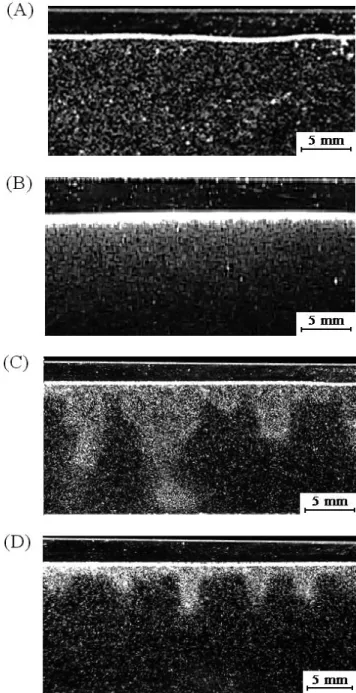
Results were obtained from a series of assays in the various Hele-Shaw set-ups described above. Bioconvection patterns recorded in horizontal view are presented in Figs. 3 and 4 and summarized in Tables 2 and 3. The TP used in our assays were in the exponential phase of growth, rather than in the steady phase. In all our assays, a uniform initial state was obtained at the initial filling time t=0 (Fig. 3A).
Three regimes of patterns formation were observed: 1) the diffusion regime; 2) the stationary convection regime; and 3) the unsteady convection regime.
Diffusion regime
We first produced a diffusion state (Fig. 3B), as pre-dicted by the mathematical model. Beginning at t=0, this state was established after 30 minutes to 2 hours, with cell concentration below the critical value for the onset of con-vection. Concentration values leading to this state ranged from 5×10⁴ to 1×10⁵ cells/cm3, depending on the dimension of the Hele-Shaw cell. Note that the profile of this diffusion state should be an exponential function (Eq. 23), but this
n b H critical= 1 2 2 1 01 102 2 2 . × b H n b H critical= × 2 6 102 2 . 2 6 103 2 . × b H
Fig. 3. Different states of bioconvection pattern. (A) Uniform initial state. (B) Diffusion state. (C) Transient state. (D) Stationary convec-tion plumes (steady state).
cannot be verified from this picture. Stationary convection regime
When the concentration was higher than a certain critical value, the diffusion state ceased to exist, and we observed the appearance of a stationary convection regime (‘P’ in Tables 2 and 3), with many small plumes very similar to those obtained by Itoh and Toida (2001) with Tetrahymena thermophila for the case with no electrical effects. Fig. 3D illustrates the steady convection patterns obtained at a con-centration n=1.27×10⁵ cells/cm3 (the dimensions of the Hele-Shaw apparatus were the same as in Assay 1 (Table 2). The time tc required for the steady state to establish varied from 30 minutes to 3 hours, depending partly on each experimental parameter set, but mostly on the initial filling concentration and the health status of the TP cells. For this
assay (Fig. 3D) tc was around 30 min. Fig. 3C illustrates a transient state before stationary convection plumes appeared.
We note, from the assays in Tables 2 and 3, that the Rayleigh numbers at which convection patterns appeared in different Hele-Shaw cells are in agreement with the numer-ical result Ra*criticital=10.2 for Pe ≥ 1 given by linear stability analysis.
Unsteady convection regime
As the concentration was increased to higher values than those leading to the “P” state described above, we observed an unsteady convection regime characterized by a collection of cloudy plumes (designated “M” in Tables 2 and 3). These plumes had non-stationary shapes, moving from side to side, dividing into small plumes and then
re-assem-Table 2. Bioconvection patterns from various Hele-Shaw apparatuses.
Number of assay [1]
Hele Shaw cell (H × L × b cm3) [2] ncritical cell/cm3 [3] n after 18 hours of incubation cell/ cm3 [4] patterns with n [5] ncentrifuged cell/cm3 [6] patterns with ncentrifuged [7]
1 4×5×0.075 1.15E+04–1.15E+05 1.50E+05 P+ 3.08E+05 P+
2 4.5×12.5×0.075 1.03E+04–1.03E+05 1.00E+05 – – 2.50E+05 P+
3 7.6×8×0.075 6.09E+03–6.09E+04 1.50E+05 P+ 3.08E+05 P+ M +++
4 9.5×6.2×0.075 4.8E+03–4.8E+04 9.00E+04 – – 1.35E+05 P+
5 16×11×0.05 6.5E+03–6.5E+04 5.30E+04 – – 1.24E+05 P+ M +++
6 18.5×11×0.04 8.78E+03–8.78E+04 1.00E+05 P+ 2.50E+05 P+ M ++
7 18.5×11×0.04 8.78E+03–8.78E+04 9.00E+04 P+ 1.50E+05 P+ M ++
8 18.5×11×0.04 8.78E+03–8.78E+04 1.50E+05 P+ 3.08E+05 P+ M+
9 4×8×0.1 6.46E+03–6.46E+04 1.92E+05 P++
10 4×8×0.1 6.46E+03–6.46E+04 1.50E+05 P+
Column (1), number of assay; column (2), dimensions of Hele-Shaw apparatus used; column (3), critical concentration of cells calculated from formula (32b), with the range of Dc=1.5×10⁻⁴–1.5×10⁻³ cm2/s; Column (4), concentration of cells obtained after 18 hours of incubation at T=24°C and pH=7.2; Column (6), concentration of cells obtained after centrifugation at 10 rpm for 5 min; Columns (5) and (7), bioconvection patterns observed in Hele-Shaw apparatuses with n and ncentrifuged, respectively. +++, very good pattern; ++, good pattern; +, faint pattern; – –, no pattern; P, stationary plumes; M, non-stationary motion.
Table 3. Bioconvection patterns from various Hele-Shaw apparatuses.
Number of assay [1] n after 18 hours of incubation cell/ cm3 [2] Peclet number Pe [3] ncentrifuged cell/ cm3 [4] Rayleigh number Ra*n [5] patterns with Ra*n [6] Rayleigh number Ra*centrifuged [7] patterns with Ra*centrifuged [8] 1 1.50E+05 120 3.08E+05 13.5 P+ 27.72 P+ 2 1.00E+05 135 2.50E+05 10.1 – – 25.3 P+ 3 1.50E+05 228 3.08E+05 25.6 P+ 52.7 P+ M +++ 4 9.00E+04 285 1.35E+05 19.2 – – 28.85 P+ 5 5.30E+04 480 1.24E+05 8.4 – – 19.8 P+ M +++ 6 1.00E+05 555 2.50E+05 11.84 P+ 29.6 P+ M ++ 7 9.00E+04 555 1.50E+05 10.65 P+ 17.76 P+ M ++ 8 1.50E+05 555 3.08E+05 17.76 P+ 36.46 P+ M+ 9 1.92E+05 120 – – 30.7 P++ – – 10 1.50E+05 120 – – 24 P+ – –
Column (1), number of assay; column (2), concentration of cells obtained after 18 hours of incubation at T=24°C and pH=7.2; Column (3), Peclet number Pe=VcH/Dc, with Dc=1.5×10⁻³ cm2/s; column (4), concentration of cells obtained after centrifugation at 10 rpm for 5 minutes; column (5), Rayleigh number Ra*n calculated from formula (25) with concentration n; Column (7), Rayleigh number Ra*centrifuged calculated from formula (25) with concentration ncentrifuged; Columns (6) and (8), bioconvection patterns observed in Hele-Shaw apparatuses with Ra*n and Ra*centrifuged, respectively. +++, very good pattern; ++, good pattern; +, faint pattern; – –, no pattern; P, stationary plumes; M, non-station-ary motion.
bling (Fig. 4). The motion of these plumes continued until the death of the Tetrahymena cells. The time tnc for this non-stationary regime to appear was about 15 to 30 minutes, depending mostly on the initial filling concentration. The plumes illustrated in Fig. 4 correspond to the third assay in
Tables 2 and 3, with a concentration of 3.08×10⁵ cells/cm3 after centrifugation, corresponding to a Rayleigh number of approximately Ra*=52.7 based on equation (25).
In the same Hele-Shaw apparatus of Assay 3, Table 2, we observed this unsteady flow for a range of
tions from 2.29×10⁵ cells/cm3 to 2.45×10⁵ cells/cm3, corre-sponding to values of the Rayleigh number Ra* varying from 39.2 to 41.9, with a dimensionless swimming speed of 228 and a diffusion coefficient Dc=1.5×10⁻³ cm2/s. We estimated that the critical Rayleigh number for the transition from steady state to unsteady state is around 40.
It may be expected that as the Rayleigh number increases gradually beyond a certain threshold, the convec-tion patterns should change smoothly from a steady to an unsteady state with a well-defined moving flow. However, it is difficult to control the various parameters necessary for this transition to occur. We instead obtained a rather cloudy pattern in Assay 3, as shown in Fig. 4, corresponding to the Rayleigh number Ra*=52.7, i.e., rather far from the esti-mated critical value Ra*c=40.
DISCUSSION
Transition to steady and unsteady flow regimes
From this experimental study, we found two critical Ray-leigh numbers for the development of bioconvection pat-terns: the first one is the value at which occurs a transition from the diffusion to the stationary convection state, as pre-dicted by linear stability theory. The second critical value corresponds to the transition from the stationary to the time-varying convection regime. The latter value could not be predicted by the linear stability analysis, but was experimen-tally estimated from Assay 3 to be about Ra*=40, i.e., four times higher than the first critical Rayleigh number, Ra*=10.2. We also found the time required for bioconvection patterns to appear, which ranged from 30 minutes to 3h for the steady regime, and 15 to 30 minutes for the unsteady regime.
In order to show the geometric effects on pattern forma-tion, we realized assays in various Hele-Shaw cells, as shown in the Table 2. We first note that when H was varied, the Peclet and Rayleigh numbers also varied proportionally. The variation in these two parameters changed the flow regime such that, at the same initial concentration, there was established a diffusion state in a Hele-Shaw cell with height H1, and a convection regime in another cell with height H2>H1.
Variation in thickness b is related to the permeability K of the porous medium by the formula K=b2/12, so that when b doubles, K quadruples and the Rayleigh number incre-ases accordingly. In other words, a small variation in b may strongly influence the convection pattern in a Hele-Shaw apparatus. It should be noted that b should not be too large to violate the 2D approximation of Hele-Shaw apparatus, nor too small to affect the motility of the microorganisms. In our study, b was always greater than 0.4 mm.
Spatial scales of pattern formation
In the steady convection regime, we observed regular plume patterns 2.5–5.5 mm long and 2.0–2.6 mm wide. The distance between two plumes was 0.4–0.8 cm at a concen-tration of 1×10⁵–3×10⁵ cells/cm3. The number of plumes depended on length L of the apparatus. These observations agree with those previously reported for TP (Plesset et al. 1976; wavelength λ=0.655 cm and average culture concen-tration=2.7×10⁵ cells/cm3). The size and distance between plumes also depended on the initial concentration, which
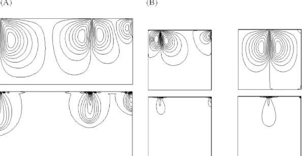
Fig. 5. Simulation results (A) Simulation time of Assay 9. (B) Sim-ulation time of Assay 3, Ra*=25.6 (after 18 hours of incubation). (C) Simulation time of Assay 3 with Ra*=52.7 after centrifugation.
may have led to unsteady patterns beyond a certain value (around 6.09×10³ – 6.09×10⁴ cells/cm3 for Assay 3). In this regime, the shape and size of the unsteady patterns were not well defined. Their speed was about 0.2–0.5 mm/s, which is of the order of the swimming speed Vc.
In interpreting these observations, we should bear in mind that bioconvection is primarily driven by the microor-ganisms, with negligible participation of the medium itself. This represents a fundamental difference with the Benard convection, in which the pattern formation is due solely to the behavior of the fluid. Plesset et al. (1976) also stressed the importance of boundaries in predicting the irregular shape of patterns, noting that “when the cells approach the surface, 17% stay in a well-defined layer at the surface. This layer has a thickness h that ranges from 1mm to 5 mm. The remaining 83% of the approaching cells are reflected from the upper layer, or from the abrupt increased cell concentra-tions in that layer”. Model predicconcentra-tions further assume that experimental cultures have uniform initial cell concentra-tions, and that the microorganisms swim with a constant upward velocity. In reality, the cells do not swim precisely in the vertical direction and with the same speed Vc. Plesset et al. (1976) therefore took the mean upward velocity to be
αVc, with α having a value slightly less than unity.
Temporal scales of pattern formation
Plesset et al. (1976) emphasized that a considerable amount of time is required before a cell turns around and resumes its normal upward swimming in the case of high concentration. Another considerable amount of time is also required to establish the convection state. If t stands for the total time required for these processes (cells turning around, and then resuming their normal upward swimming and reaching the convection state), we observed in our experi-ments that t was around 30 minutes to 3 hours for the steady convection regime, depending on the geometry and initial filling concentration (i.e., the Rayleigh and Peclet
num-bers). In the case of the unsteady regime (Fig. 4), the amount of time for the cloudy patterns to appear was around 15–30 minutes, depending on the Rayleigh and Peclet num-bers of the system, but the time required to reach a final steady state was infinite.
We note in passing that the dimensional time t* was cal-culated from t*=tH2/Dc, where t was the dimensionless time used in the numerical simulations shown in Figs. 5 and 6. For Ra=30.7, t*=10.666×10³ s ≈ 3 h (Figs. 5A and 6A). For Ra=25.6, t*=7.8×10³ sec ≈ 2 h (Figs. 5B and 6B). For Ra=52.7, t* obtained from simulation was infinite, i.e., the numerical calculations could not reach any steady state, as illustrated by the streamlines and iso-concentration lines at t=1 (corresponding to t *≈1 h) (Figs. 5C and 6B).
Population dynamics and pattern formation
Under optimal conditions, the growth of TP is character-ized by a logarithmic growth phase, a pre-stationary growth phase, and a stationary phase. In the logarithmic phase, which may last from a few hours to a couple of days, depending on the inoculum, cell density increases logarith-mically, the generation time being 3–7 h. In the pre-station-ary phase, growth decreases for a few generations before entering the last stationary phase (Sauvant et al., 1999).
If the growth rate is taken into account, there will be a significant effect of density growth on pattern formation, because the concentration and Rayleigh number will both increase. We so far have assumed that the coefficient of dif-fusion Dc and the swimming speed Vc are constant. How-ever, there may be an important effect of collisions between cells as density increases, and both Dc and Vc may vary. Such systems could be strongly influenced by the coupling between nonlinear processes of transport and growth. From studies of diffusive instabilities and pattern formation in pop-ulations (Okubo and Levin, 2002), it may be expected that the time scale of population growth relative to the convection time should be of critical importance in predicting spatial
het-Fig. 6. Streamlines (above) and isoconcentration lines (below), from numerical study with a mesh of 61×61 nodes. (A) Case of Assay 9: Pe=120, Ra*=30.7, t=1. (B) Case of Assay 3: Pe=228, Ra*=25.6, t=0.3 (left) and Pe=228, Ra*=52.7, t=1 (right).
erogeneity in dynamic populations. This multi-scale and nonlinear nature of bio-physical problems remains one of the most challenging difficulties in self-organized phenom-ena in ecological and evolutionary systems.
CONCLUSION
We used the Hele-Shaw apparatus as a model system to study 2D bioconvection phenomena in Tetrahymena pop-ulations. We successfully produced a transition from the dif-fusion state to stationary bioconvection, as predicted by the stability analysis, and we determined the temporal scales associated with pattern formation. Furthermore, the Hele-Shaw apparatus also showed the transition to unsteady flow regimes. Further studies at high Rayleigh and Peclet num-bers are necessary to better understand the spatio-temporal development of this time-varying bioconvetion.
ACKNOWLEDGMENTS
TNQ thanks Prof. N. Lima (Centre for Biological Engineering, University of Minho, Braga, Portugal) for his precious support and Prof. M.P. Sauvant Rochat (Cellular Biology Lab., Université d’Auvergne, France) for her collaboration. We especially thank Mrs. Laviolette (Ecole Polytechnique de Montreal, Canada), and Mr. Morency and Mrs. Phoenix (University of Montreal, Canada), for their kind assistance. FG acknowledges support from the James S. McDonnell Foundation through a 21st Century Science Initiative award. We thank an anonymous reviewer for his interesting com-ments.
REFERENCES
Assar H (1988) Effect of cadmium, pentachlorophenol and light on bioconvection patterns in Chlamydomonas reinhardtii. Master’s Thesis, Department of Biology, University of Montreal, Montreal Bahloul A, Nguyen-Quang T, Nguyen TH (2005) Bioconvection of
gravitactic microorganisms in a fluid layer. Int Commun Heat Mass 32: 64–71
Bamdad M (1991) Étude de la Toxicité de la Nigéricine, Antibiotique Polyéther Carboxylique, en Relation avec ses Propriétés Iono-phores, sur le Protozoaire Cilié Té trahymena pyriformis. Thèse de Doctorat, Département de Biologie, Université Blaise Pas-cal, Clermont Ferrand, France
Childress S, Levandowsky M, Spiegel EA (1975) Pattern formation in a suspension of swimming micro- organisms: equation and stability theory. J Fluid Mech 63: 591–613
Czirok A, Janosi IM, Kessler JO (2000) Bioconvective dynamics dependence on organism behaviour. J Exp Biol 203: 3345– 3355
Darcy HP (1856) Les Fontaines Publiques de la ville de Dijon. Vector Dalmont, Paris
DeLuca EE, Werne J, Rosner R, Cattaneo F (1990) Numerical simu-lations of soft and hard turbulence: Preliminary results for two-dimensional convection. Phys Rev Lett 64: 2370
Hele-Shaw HJS (1898) On the motion of a viscous fluid between two parallel plates. Nature 58: 34–36
Itoh A, Toida H (2001) Control of bioconvection and its mechanical application. IEEE/ASME International Conference of Advanced Intelligent Mechatronics, 8–12 July, Como, Italy, pp 1220–1225
Janosi IM, Czirok A, Silhavy D, Holczinger A (2002) Is bioconvection enhancing bacterial growth in quiescent environments ? Envi-ron Microbiol 4: 525–532
Kessler JO (1986) Individual and collective fluid dynamics of swim-ming cells. J Fluid Mech 173: 191–205
King JR (2001) Two generalisations of the thin film equation. Math Comput Model 34: 737–756
Kowalewski U, Braeucker R, Machemer H (1998) Responses of Tetrahymena pyriformis to the natural gravity vector. Micro-gravity Sci Tech 11: 167–172
Kramhøft B, Lambert IH (1997) Taurine transport systems in the ciliate protozoan Tetrahymena pyriformis. Amino Acids 12: 57– 75
Loefer JB, Mefferd RBJ (1952) Concerning pattern formation by free swimming microorganisms. Am Nat 86: 325–329
Malchow H, Petrovskii S, Medvinsky A (2001) Pattern formation in models of plakton dynamics. A synthesis. Oceanol Acta 24: 479–487
Mogami Y, Yamane A, Gino A, Baba SA (2004) Bioconvective pat-tern formation of Tetrahymena under altered gravity. J Exp Biol 207: 3349–3359
Nguyen-Quang T (2006) Gravitactic Bioconvection Study in Porous Media (Etude de la Bioconvection gravitactique en Milieux poreux) PhD Dissertation, Department of Mechanical Engineer-ing, Ecole Polytechnique de Montréal, University of Montreal, Montreal
Nguyen-Quang T, Bahloul A, Nguyen TH (2005) Stability of gravi-tactic micro-organisms in a fluid-saturated porous medium. Int Comm Heat Mass 32: 54–63
Okubo A, Levin S (2002) Diffusion and Ecological Problems: Mod-ern Perspectives. 2nd ed, Springer, New York
Pedley TJ, Kessler JO (1992) Hydrodynamic phenomena in suspen-sions of swimming micro-organisms. Ann Rev Fluid Mech 24: 313–358
Platt JR (1961) Bioconvection patterns in cultures of free-swimming organisms. Science 133: 1766–1767
Plesner P, Rasmussen L, Zeuthen E (1964) Techniques used in the study of synchroneous Tetrahymena. In “Synchcrony in Cell Division and Growth” Ed by E Zeuthen, Intersciences, New York, pp 534–565
Plesset MS, Winet H (1974) Bioconvection patterns in swimming micro-organism cultures as an example of Rayleigh-Taylor instability. Nature 248: 441–443
Plesset MS, Whipple CG, Winet H (1976) Rayleigh-Taylor instability of surface layers as the mechanism for bioconvection in cell cul-tures. J Theor Biol 59: 331–351
Reinelt DA (1987) The effect of thin film variations and transverse curvature on the shape of fingers in a Hele–Shaw cell. Phys Fluids 30: 2617–2623
Sauvant MP, Pepin D, Piccini E (1999) Tetrahymena pyriformis, a tool for toxicological studies. A review. Chemosphere 38: 1631– 1669
Wager H (1911) On the effect of gravity upon the movements and aggregation of Euglena Viridis, Ehrb., and other micro-organisms. Philos Trans R Soc Lond B 201: 333–390
Nomenclature
b thickness space between two plates, mm
Dc cell diffusivity, m2/s
F=L /H aspect ratio of 2D porous cavity
gravitational acceleration, m2/s
k wave number
kc critical wave number
K permeability of porous medium, m2
n(X,Y,Z,t*) cell concentration, cells/m3
–n mean cell concentration in a cavity of length L, height H, and depth W, , cells/m3.
n0 cell concentration at the lower boundary Y=0, cells/m3 n1 cell concentration at the upper boundary Y=H, cells/m3 N=(n–n0) /∆n dimensionless cell concentration
–
N=(–n–n0) /∆n dimensionless mean cell concentration (at t=0)
P* dynamic pressure, Pa
P=H2P*/ρ 0Dc2 dimensionless pressure Ra=g–nb2Hβ Pe/12νD
c Rayleigh number
Ra*=Ra/Pe=g–nb2Hβ /12νDc renormalized Rayleigh number
Rac critical Rayleigh number
Darcy velocity, m/s gravitactic cell velocity, m/s dimensionless Darcy velocity dimensionless cell velocity
(X,Y, t*) Cartesian coordinates, m, and time, s
(x,y, t) dimensionless coordinates x=X/H; y=Y/H, and time t=Dct*/H2 Greek symbols
β=ϑ∆ρ /ρ0 density variation coefficient of suspension ∆ρ = ρc– ρw difference of cell and water densities, kg/m3 ψ =ψ */Dc dimensionless stream function
ν kinematic viscosity of the suspension, m2/s
ρw water density, kg/m3
ρc cell density, kg/m3
ρ density of suspension “fluid-cell’’, kg/m3
ρ0 suspension density at the bottom, kg/m3
ϑ cell volume, m3/cell
G g n WLH dZ dX n X Y Z t dY W L H = 1