Development and validation of a single mass Lap simulation

Development and Validation Of a Single Mass Lap

Simulation

by

Jeremy R. Noel

Submitted to the Department of Mechanical Engineering

in partial fulfillment of the requirements for the degree of

Bachelor of Science in Mechanical Engineering

at the

MASSACHUSETTS INSTITUTE OF TECHNOLOGY

May 2020

c

○ Massachusetts Institute of Technology 2020. All rights reserved.

Author . . . .

Department of Mechanical Engineering

May 8, 2020

Certified by . . . .

Ian Hunter

George N. Hatsopoulos Professor in Thermodynamics

Thesis Supervisor

Accepted by . . . .

Maria Yang

Professor of Mechanical Engineering

Development and Validation Of a Single Mass Lap Simulation

by

Jeremy R. Noel

Submitted to the Department of Mechanical Engineering on May 8, 2020, in partial fulfillment of the

requirements for the degree of

Bachelor of Science in Mechanical Engineering

Abstract

In this thesis, a single mass model lap time simulation was designed, implemented and validated in MATLAB. The goal of this simulation was to accurately predict the velocity of a formula style open wheeled race car on a given track. The simulation was constructed in MATLAB, and features a function based design that will allow the core algorithm to be used with more sophisticated vehicle models. The code was tested and validated using a combination of contrived and collected map data, and a strong correlation of 0.8067 was shown with 95% confidence bounds of 0.8028, and 0.8105. Finally, this thesis outlines proper testing techniques to obtain the data required to complete the validation process of this simulation.

Thesis Supervisor: Ian Hunter

Acknowledgments

There are so many people I would like to thank who have made this research and development project possible. First, of course are my parents and aunt, without whose support and constant requests to please get my stuff out of their garage, I would not have found my passion for vehicle design. Next are the former leaders of the FSAE team, in particular Luis Mora, Cheyenne Hua and Elliot Owen who showed incredible patience with me as I made enough foolish mistakes to learn for myself just how hard developing a a functional car can be. Then are my own FSAE cohort, who made my four years on the team the best possible experience. I thank my friends for putting up with me living in shop for most of my four years, and especially Elizabeth Harkavy for her Latex and editing help. Finally I would like to thank Dr. Christopher Vick, without whom I would never have found myself at MIT. I consider myself truly fortunate to stand on the shoulders of these giants.

Contents

1 Introduction 13

1.1 Formula SAE Competition . . . 13

1.2 Team Background . . . 14 1.3 Motivation . . . 15 1.4 Objective . . . 16 1.5 Previous Simulations . . . 16 2 Design Of Simulation 19 2.1 Vehicle Model . . . 19 2.2 Simulation Design . . . 20

2.3 Coordinate systems, and Units . . . 20

2.4 Assumptions . . . 21

2.5 High level code structure . . . 22

2.6 Subsystem Functions . . . 24

2.6.1 Car Parameters . . . 24

2.6.2 Path Generation Techniques . . . 24

2.6.3 Splitting the Lap into Segments . . . 29

2.6.4 Driver Vision . . . 32

2.6.5 Driving Function . . . 33

2.7 Data Visualization . . . 41

2.7.1 Velocity Plot . . . 41

3 Validation 43

3.1 Validation Goals . . . 43

3.2 Validation Structure . . . 43

3.3 Creating Useful Test Cases . . . 44

3.3.1 Acceleration Run Test Case . . . 44

3.3.2 Constant Radius Turn . . . 47

3.3.3 Variable Radius Turn . . . 50

3.4 Utilization of Testing Data . . . 51

3.4.1 Small Map Testing . . . 51

3.4.2 Full Lap Testing . . . 52

3.5 Next Steps for Validation . . . 54

3.5.1 Testing Procedure for Simulation . . . 54

3.5.2 Testing Sweeps to Ensure Predictive Nature . . . 55

4 Conclusion 57 4.1 Future Work . . . 57

List of Figures

1-1 High level block diagram of acceleration simulation [4] . . . 17

2-1 Vehicle axis system [10] . . . 21

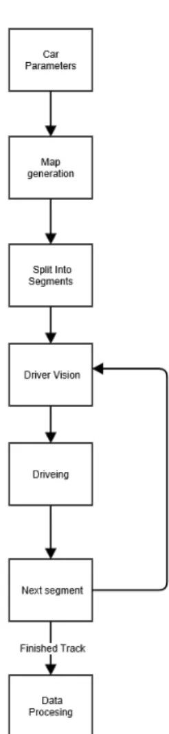
2-2 High level block diagram of code structure . . . 23

2-3 Image provided by SAE depicting a single autocross lap [8] . . . 25

2-4 Overlay of extracted points over the original map . . . 25

2-5 A car weaves through an autocross slalom section similar to an FSAE track [1] . . . 27

2-6 Overlay of three different gaussian smoothing windows . . . 28

2-7 Determining radius and angle from a series of points [3] . . . 29

2-8 Lap times of 1000 iterations of random segment locations compared to calculated segments . . . 31

2-9 Example of a simple map split into three segments . . . 32

2-10 element velocity plot in back step solving . . . 40

2-11 Final element velocity plot in back step solving . . . 40

3-1 Model of standard FSAE acceleration track . . . 45

3-2 Velocity of the car on a straight track shown as a function of distance 46 3-3 Velocity of the car on a straight track shown as a function of distance 47 3-4 Map created using debugging map creator with straights and a constant radius . . . 48

3-5 Compettiont skidpad course[7] . . . 49

3-6 The velocity plotted against the distance traveled comparing the sim-ulation to competition results . . . 50

3-7 Velocity of the U-Turn map . . . 50 3-8 The velocity plotted against the distance traveled . . . 51 3-9 Velocity of the Variable radius U-Turn map . . . 51 3-10 The velocity plotted against the step number overlayed with testing data 53 3-11 Velocity shown as colors on the practice map . . . 53 A-1 The velocity plotted as a function of time overlayed with endurance data 60 A-2 Velocity shown as colors on the endurance map . . . 60 A-3 The velocity plotted against the step number overlayed with testing data 60 A-4 Velocity shown as colors on the practice map . . . 60 A-5 The velocity plotted against the step number overlayed with testing data 61 A-6 Velocity shown as colors on the practice map . . . 61 A-7 The velocity plotted against the step number overlayed with testing data 61 A-8 Velocity shown as colors on the practice map . . . 61

List of Tables

1.1 FSAE Competition Points Breakdown . . . 14 2.1 Car Parameters . . . 24

Chapter 1

Introduction

1.1

Formula SAE Competition

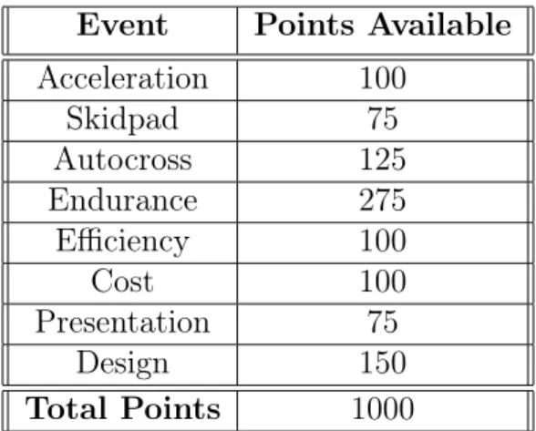
The Formula SAE (FSAE) Competition is a collegiate design competition where students deign, build and race an open wheel formula-style racecar. The competition has a series of scored events. These events consist of two separate categories, dynamic and static, and when combined they create a total score upon which a winner is de-cided. The dynamic events test the performance of the car in straight line acceleration (75m drag race: 100 points), skidpad (steady state cornering on a dry surface: 75 points), autocross (single lap around a cone track: 125 points) and endurance (22km auto-cross that includes a change of driver at the midpoint: 275 points plus efficiency: 100 points). The dynamic events make up a total of 675 points [7]. The static events seek to reward excellence in engineering knowledge as well as design decisions. There are three events: cost (points awarded based on proper book keeping and overall cost: 100 points), presentation (a mock business presentation highlighting logistics, production and technical advancement: 75 points) and design (evaluation of engi-neering effort, design goals and overall comprehension of the team: 150 points) [7]. The static events make up a total of 325 points. The competition is a race to collect as many of the 1000 available points as possible. The point breakdown is summarized in table 2.1.

Table 1.1: FSAE Competition Points Breakdown

Event Points Available Acceleration 100 Skidpad 75 Autocross 125 Endurance 275 Efficiency 100 Cost 100 Presentation 75 Design 150 Total Points 1000

The FSAE competition originated in 1981, and consisted of a total of 6 teams [2]. The internal combustion (IC) competition rapidly grew and now has multiple compe-titions across the United States. In 2013 the first electric variant of the competition was introduced with a partial set of rules. This competition featured 20 registered teams of which 9 made it to the actual competition[9]. In a similar swell the electric competition is now flourishing with the 2019 competition boasting 30 registered teams with 27 making it to competition. 2020 will mark the first year that FSAE has not hosted an in person competition since its inception, due to the COVID-19 pandemic.

1.2

Team Background

MIT Motorsports is an FSAE team that competes annually in the electric class. The team is made up of about 40 students who are a mix of mechanical, electrical and software engineers with the occasional business minded student leading the charge to raise enough money to stay afloat. The team is entirely student run, and is led by a few adventurous juniors, who are in way over their heads.

MIT Motorsports began in 2001, a small team lead by Nick Gidwani who led the team to build the first IC car. The team grew and climbed the ranks of the IC competition, culminating in a 16th place finish out of 105 teams competing in 2012. The team then transitioned to the electric competition, and in 2015 successfully built

the first electric racecar that ran, although not in time to compete. The team’s performance grew quickly, culminating in a dominant performance in 2018, when the team was disqualified after winning the endurance race by over a minute, due to an alleged overpower event.

This success led the team to try to grow further for the model year 2019 car (MY19). It was determined that the most effective way to score the required number of points to win would be through a four wheel drive (4WD) architecture. This deci-sion was primarily made with the preexisting simulation tools the team had available. The primary simulation tool was a single mass ordinary differential equation (ODE) based acceleration simulation. This simulation and its limitations will be discussed at length in section 1.5. Ultimately the MY19 car proved to be too much to handle in a single year. Both the attempt at a revolutionary new liquid cooled battery pack and a 4WD car failed. The team was still able to compete with a rear wheel drive (RWD) car and a hastily made air cooled battery pack. Still the team found some success with good performances in both acceleration (2𝑛𝑑_{) and skidpad (3}𝑟𝑑_{), but did}

not complete autocross, and finished out of the top three in endurance.

Ultimately MIT Motorsports maintains its status as a yearly contender for the elusive first place prize. The team was hungry in MY20, learning from the mistakes made in the previous year and building a more conservative car on an aggressive time-line. This strategy seemed to be paying off before the season was cut short. The team remains hungry as a new design and build cycle begins for MY21.

1.3

Motivation

The primary motivation for this project was to establish stronger simulation tools for architecture decisions for future design cycles of the MIT Motorsports FSAE vehicle. The simulation developed in this thesis will help the team to rapidly weigh the overall effects of different architectures in all dynamic events. This simulation will also aid in the static score through providing more accurate point estimations and justifications for design decisions.

1.4

Objective

The objective of this thesis is to establish the framework of a full lap simulation specific to an FSAE electric race car. This simulation should be able to accurately predict the behavior of an FSAE car at its tractive limit at all times. The simulation should also be able to provide other key parameters about the lap, ranging from maximum speed, to maximum power, and total power consumed. All of these outputs can help to determine sensitivities to a variety of car parameters. This project also seeks to outline a testing procedure and tests necessary to build a database to be able to fully validate the simulation across a variety of conditions. In summary there are four primary objectives for this project:

1. Create a lap time simulation that can take several input formats, including GPS data, picture style maps, and arbitrary user defined maps. The simulation must then generate a velocity map as well as other parameters of interest including power and acceleration.

2. Ensure that the core algorithm used for solving for the behavior of the car is compatible with more detailed vehicle models such as a bicycle model, and a two track model.

3. Validate the model with existing data to ensure that the model performs both logically and matches the data.

4. Outline a testing platform and procedure that will allow the fidelity of the model to increase as the team is able to collect additional data from the car.

1.5

Previous Simulations

The team has developed and used multiple versions of a linear acceleration sim-ulation. The first iteration was an ODE based solver that utilized a single mass model. A high level block diagram of this code is shown in figure 1-1. This was a suitable simulation for design decisions but did not feature the separation required

for testing launch control algorithms in the code. This code was advanced in 2019 with a Simulink based acceleration simulation that did feature an independent con-trol system[4]. Many of the features in the lap simulation were based on the concepts displayed in this Simulink model.

Figure 1-1: High level block diagram of acceleration simulation [4]

The tremendous growth and technical advancements attempted by the team in 2019 made painfully obvious the lack of advanced simulation tools available to make those decisions. The team had focused primarily on the acceleration model when making the 4WD architecture decision. The acceleration model was supplemented by the use of Optimum Lap (a commercial lap simulation software). The nature of Optimum Lap as a single mass model does not allow for explicit specification of 4WD vs RWD. It does, however, provide some basis for how the car will perform in a dynamic sense. The use of an acceleration simulation as the primary simulation led to an overemphasis on the straight line capability of the car. The straight line acceleration is a place where 4WD is excellent, and the simulation did not properly penalize higher vehicle mass and unsprung mass.

The use of Optimum Lap was the first step in the correct direction. Optimum Lap is a single mass model much like the one developed in this thesis. While the Optimum Lap results are useful when no other simulation is available, the inability to refine the code makes for a less than ideal option. Additionally Optimum Lap struggles to accurately model complex lap shapes, which created issues for the team

in the 2019 build cycle. This may lead to results that do not make sense, or worse, can be misleading.

Chapter 2

Design Of Simulation

2.1

Vehicle Model

This simulation models the vehicle as a single mass with several known parameters. These parameters include the coefficient of friction of the tire with the road surface, the drag and lift coefficients (𝐶𝐷𝐴 and 𝐶𝐿𝐴), vehicle mass and the drive-train

pa-rameters. This vehicle model assumes that the vehicle has a tractive capability that comes from the normal force at the tire patch and the coefficient of friction, shown in equation 2.8. This tractive capability can either be used to generate lateral or longitudinal acceleration.

This model has some significant drawbacks. First, with a RWD car, only the tractive capability of the rear wheel is able to generate longitudinal acceleration. With the single mass model there is no discrimination between front and rear wheels, which means this model is unable to accurately differentiate between 4WD and RWD. Similarly the way that lateral acceleration is generated by the car requires knowing the steering angle, as well as the slip ratio of the tire. Again this is simplified to just tractive capability of the imaginary single tire with this model. Despite the simplistic nature of this model the predictive results that can be achieved are still impressive.

2.2

Simulation Design

This simulation works by taking a map that is a series of elements that contain information about both the length of the element and the radius of the turn that it approximates. From this data the simulation splits these elements into segments which contain one turn each. This segment is then split into two further subdivisions around the apex of of the turn, which is defined as the minimum radius element, and is therefore the minimum speed of the turn. From this point the simulation uses backwards distance steps to solve for the velocity of all elements before the apex, and forward distance steps for all elements that are after the start point. This creates a segment that is made up elements that are continuous in velocity.

Once a segment’s velocity has been determined the segment is added to all the previously solved segments. Continuity of velocity is then checked over these elements. If the velocity is continuous the simulation moves onto the next segment. If it is not, the previous segment is resolved starting at the new segment velocity until a continuous velocity profile is created. This method allows the effective generation of a complete velocity profile for a given map.

2.3

Coordinate systems, and Units

The global coordinate system for this model is based on the generated map. This global coordinate system is a 2D XY plane, where the start and end points are arbitrary. It is important to note that all altitude change is ignored. The origin of the global coordinate system is arbitrarily determined to allow the entire track to be in the first quadrant. On this global coordinate system a car coordinate system can be mapped using the standard SAE format, which is shown in figure 2-1[5]. Positive X is the forward facing vector, positive Y is the right pointing vector and Z is a downward vector. Leading to forward acceleration, gravity, and turning right all produce positive accelerations in the car reference frame. Roll, pitch and yaw describe the rotation of the car about the same set of axes. The origin of the car is

defined at the center of gravity, which is convenient for this model because it allows no generation of moments.

Figure 2-1: Vehicle axis system [10]

2.4

Assumptions

This simulation is based on a series of assumptions which are listed and commented on below.

1. There is no significant change in altitude during the course of a lap 1

2. At the tightest radius in a turn, a car traveling at its maximum possible velocity will be in purely lateral acceleration2_.

3. Each element is a distance step and the car’s velocity is a linear approximation from the velocity at the beginning of the element (𝑉𝑖𝑛) to the velocity at the

end of the element (𝑉𝑜𝑢𝑡). Furthermore the 𝑉𝑖𝑛 of an element is equal to the

𝑉𝑜𝑢𝑡 of the previous element, and 𝑉𝑎𝑣𝑒 is defined by equation 2.1.3.

𝑉𝑎𝑣𝑒 =

𝑉𝑖𝑛+ 𝑉𝑜𝑢𝑡

2 (2.1)

1_{This assumption proves to be good during the annual FSAE competition but will provide some}

problems during normal testing of the car. The track that the car is tested at (Palmer Motor-sports Park), features significant altitude change. This will have to be addressed through careful consideration of the data collected

2_{This assumption is the catalyst for how the simulation handles corners, and is found to be both}

intuitively true and well supported based on GPS data.

4. The brakes can always provide more force than the tires can transmit to the ground4_.

5. The coefficient of friction between the tire and the ground is constant5.

2.5

High level code structure

This simulation is built using a series of MATLAB functions that are called in series and in loops in an overall MATLAB code. This structure provides a lot of flexibility which is essential to this project, as the future of this simulation will uti-lize more sophisticated vehicle models within the same framework. This architecture allows more complicated vehicle models for longitudinal and lateral dynamics to sim-ply be dropped into the functions that govern the car’s dynamics. A function based structure also allows for effective debugging of components of the code independently. Finally the structure helps to simplify the overall code by allowing the easy reuse of functions in different locations.

The overall simulation follows a series of steps that is very intuitive, and similar to how a driver would approach racing on a given track. The first step is to create a path for the car to follow, and this process is described in section 2.6.2. The map then gets split into segments, which are each defined as a single turn. A turn can vary widely in how it affects car velocity, from a slalom section, where a very slight turn is required, to a hairpin, in which the car will slow almost to a crawl and make a full 180∘ turn. The splitting of the map into segments is described in section 2.6.3. The next step is to identify the apex (defined by the assumptions) of the turn. This function examines one segment at a time and identifies the slowest part of the turn. This function is described in section 2.6.4. The slowest part of the turn will be the

4_{This is an excellent assumption, because the FSAE rules require that the car pass a brake}

test. The brake test consists of the car accelerating, then breaking hard, until all 4 tires perform a "lockup"[7]. This is a demonstration that the brakes are capable of overcoming the tractive capability of the car.

5_{This assumption is an okay place to start but does not accurately model the tires, which have}

a load sensitivity that will change the coefficient of friction based on the force applied[11]. This is something that can be added to a future vehicle model.

starting point for the next section, which will actually handle the determination of velocities at each element. This is the most complicated function and is actually made up of several subsections to handle all of the different possible cases. Ultimately this is the heart of the code that will handle the longitudinal and lateral dynamics of the car at each time step, and is described in section 2.6.5. Finally the user can develop any set of data visualization tools that are helpful. Two examples are included in section 2.7. This whole structure is shown in figure 2-2.

2.6

Subsystem Functions

2.6.1

Car Parameters

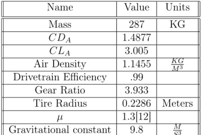
The car parameter generation function creates a struct MATLAB variable that encodes all of the different aspects used to describe the car. This could also be done by simply saving this struct as a .mat file and loading it. By instead utilizing a function, the simulation allows the user to implement parameter sweeps within the code without having to manually change the parameter of interest every time. For all of the testing that was conducted for this project the parameters were not changed. The parameters and the values used are shown in table ??

Table 2.1: Car Parameters

Name Value Units

Mass 287 KG 𝐶𝐷𝐴 1.4877 𝐶𝐿𝐴 3.005 Air Density 1.1455 𝐾𝐺_𝑀3 Drivetrain Efficiency .99 Gear Ratio 3.933

Tire Radius 0.2286 Meters

𝜇 1.3[12]

Gravitational constant 9.8 _𝑆𝑀3

2.6.2

Path Generation Techniques

There are many ways to create a map for a simulation. Each has its own merits and use cases. In this project I include and use three different techniques that provide varied sources from which simulations can be run.

Picture Data Processing

One map generation technique that is particularly useful is the ability to take a picture and convert it to a point cloud. This is useful because the FSAE competition

provides teams with maps for all dynamic events before the competition in the student handbook [8]. These images can be found online for many different competition locations and years. This data-set also comes paired with competition results which include the times and some basic vehicle parameters for each car in each event. The time of each car in each event gives the most basic data point for a simulation check which will be used in section 3.3. Additionally, MIT Motorsports has data from logging at competition for many of the years we competed in dynamic events.

The function described in this section takes a picture, like the one shown in figure 2-3, and looks for a certain color. For this particular map it is a light purple. The code looks through the image and identifies all the locations of the light purple color, and records their pixel coordinates. This mapping can then be overlayed onto the original picture as an effective way to check the code. This is shown in figure 2-4. One important note is that the image is a mirror of the original image. This will have no effect on the actual quality, so there is no point in mirroring the original image to alleviate this.

Figure 2-3: Image provided by SAE de-picting a single autocross lap [8]

Figure 2-4: Overlay of extracted points over the original map

There is now a point cloud of the map stored as global X and Y positions. This point cloud will require some post processing before it can be useful to the simulation. The first step is the conversion of a rasterized point cloud (an artifact of how it was obtained), to a sequenced series of points that describe the path the car will follow. This is done by determining a start point, then finding the closest point, and then repeating the process. This generates a sequenced series of points, which appear the same as figure 2-4, but will now be correctly ordered.

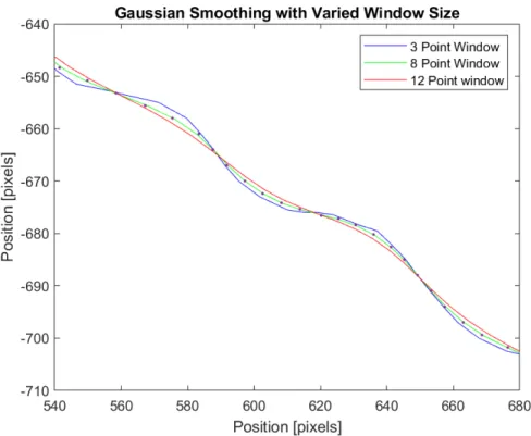
The final step is to apply some smoothing to the point cloud, which is essential because the simulation is sensitive to small deviations in point position. The im-portance of this will become evident in section 2.6.3. This is done using a Gaussian smoothing function, and the fit is selected by the user. The current process is to plot several different smoothed overlays, and then to select the one that appears to best capture the map without losing details. This is especially important in features like a slalom, shown in figure 2-5, where the movement of the car is small, but has a large effect on the allowable speed of the car. This series of different sized smoothing windows is overlayed, so that the user can make a determination. An example of this overlay is shown in figure 2-6.

The final step is to perform a dilation, which is a unit conversion from pixels to meters. The scale is easily determined by measuring the scale provided on the FSAE track in pixels. The culmination of all of these steps leads to a completed point cloud map that is a faithful representation of what was raced at competition. This can be compared to the actual autocross length which is given as approximately 800 meters [8]. The picture conversion tool is most useful when looking back at old tracks, where the team did not compete or does not have GPS data. This ability allows the team to get an idea of how they would have performed in dynamic events at competitions that the team was unable to attend.

Debugging Map Creator

The debugging map creator is an essential tool for debugging and verification of the simulation. This is by far the simplest map generation tool, and can be used to

Figure 2-5: A car weaves through an autocross slalom section similar to an FSAE track [1]

create simple, very clean point clouds in almost any shape. The maps generated that are particularly useful are straight line acceleration, semicircle, and sin functions. The debugging map creator provides the highest quality output, where the segmenter is able to produce very smooth radius estimations without smoothing. The drawback of this method is that all of the track attributes must be coded by hand, therefore to create a function that accurately represents lap data would take considerable time. Consequently, this tool is best used for simple track configurations where the creation is intuitive.

Testing Data

The final tool for creating a map is to use logged GPS data from the car. This tool is important because it is the only tool that is paired with real car data, which is essential for validation. This data-set does present some large challenges in preparing the map for the simulation, and also presents some problems with the assumptions made. The largest challenge is the accuracy of the GPS coordinates. The GPS position is coupled with an accuracy, and if the accuracy degrades then the points can begin to create shapes that the car did not actually follow. The simulation however will follow these points, creating a discrepancy. This issue will be addressed with smoothing. The larger issue is that the car while driving a lap will often slip. One of the core assumptions in this code is that the car does not slip. The slipping

Figure 2-6: Overlay of three different gaussian smoothing windows

will cause the car to create a map that has a velocity value that is not attainable in the simulation. This can be partially addressed by smoothing, but not completely. The best way to alleviate this issue is to modify the way that testing is performed. This modified testing approach is described in section 3.5.1.

The first step in converting the testing data is to extract the data from the car’s vehicle control unit (VCU), which is then converted to a .mat file, and uploaded to the team server. This data will require a unit conversion as it is recorded in longitude and latitude coordinates. The conversion is done using equation 2.3, providing position of all of the points relative to one another, and normalizing them by subtracting the lowest value. 𝑋 = 𝑅𝑒𝑎𝑟𝑡ℎ× 𝑙𝑜𝑛𝑔𝑖𝑡𝑢𝑑𝑒 × 10 −7_{× 𝜋} 360 − 𝑚𝑖𝑛(𝑋) (2.2) 𝑌 = 𝑅𝑒𝑎𝑟𝑡ℎ× 𝑙𝑎𝑡𝑖𝑡𝑢𝑑𝑒 × 10 −7_{× 𝜋} 360 − 𝑚𝑖𝑛(𝑌 ) (2.3) 𝑅𝑒𝑎𝑟𝑡ℎ = 6371000 Meters

laps. This can be done by plotting the longitude against time and finding the point at which the line goes over the same longitude. This task is extremely simple and will only have to be done once per data-set. This step will also serve as a trimming step, where the ends of the data are trimmed such that there are not long portions of time where the car is not moving. This is particularly important because if the car is not moving it can result in elements that have a length of zero which would create a singularity.

The resulting point cloud at this stage is very similar to the PNG output after being correctly ordered. Therefore the same smoothing techniques will be used here, resulting in a finished data-set.

2.6.3

Splitting the Lap into Segments

Now that a map has been generated, the map has to be converted into elements. The first part of this code is to calculate the radius that is created by each set of three points. This process is done using equations described in Lap Time Simulation, which is summarized below, and which reference figure 2-7[3].

Figure 2-7: Determining radius and angle from a series of points [3]

𝑃 = 360 − 2𝐴

R (the radius of point A) can then be determined using sin rules. R is the most important output, it describes the radius of the turn the car is making at each element. This formulation is particularly helpful because it is easy to assign a radius to each sequential point in the determined map. This means that by creating a looping function a radius is assigned to each point and stored.

sin 𝑃 = 𝑎 2𝑅 𝑅 = 𝑎 2 sin 𝑝 𝑅 = 𝑎 2 sin 180 − 𝐴 (2.5)

The next step is to calculate the angle that the three points make. This angle will serve to determine where each of the turns starts and ends, and will also help future simulations determine a steering angle. Angle A can be solved for using the cosine rule.

𝐴 = 𝑐𝑜𝑠−1(𝑏

2_{+ 𝑐}2_{− 𝑎}2

2𝑏𝑐 ) (2.6)

Another aspect that needs to be extracted from the map points is the distance between every point. Depending on the format and level of conditioning of the data, this could be a constant or varied distance. The simulation will require a certain element size to reach an acceptable level of accuracy. The distance between each step will be easy to calculate, with a little help from an old friend, Pythagoras.

𝑑 =√︁𝑑𝑥2_{+ 𝑑𝑦}2 _(2.7)

𝑑𝑥 = 𝑥(𝑛) − 𝑥(𝑛 − 1) 𝑑𝑦 = 𝑦(𝑛) − 𝑦(𝑛 − 1) 𝑛 = 𝑒𝑙𝑒𝑚𝑒𝑛𝑡 𝑖𝑛𝑑𝑒𝑥

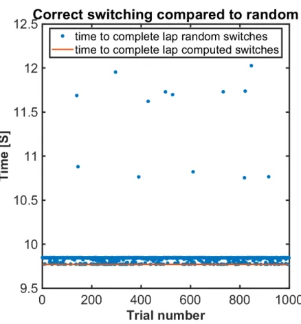
The last value that needs to be determined is the beginning and end of each turn. These values will be used to determine the segment size that is passed into the ac-tual driving function. This process is relatively simple and compares the angles of neighboring elements to determine where each turn begins and ends. This requires some rounding to prevent small osculations around zero from triggering creation of multiple segments. The importance of the segmenting goes back to section 2.5. If the segments do not capture the entirety of a curve then the code will not perform as efficiently, because the driver function will have to run multiple times over the same section and recalculate points. Poor placement will also have adverse effects on the calculated lap time.This was proven by selecting the switches randomly, instead of by the angle change. The random switch selection is repeated a thousand times and the various resulting lap times were plotted compared to the correct selections in figure 2-8.

Figure 2-8: Lap times of 1000 iterations of random segment locations compared to calculated segments

The segmenter has taken a map and converted from a point cloud to a series of elements with known length and radii. These elements were then split into segments that represent individual turns. This format will be used for all of the proceeding simulation computations. The only other time the point cloud will be used is for visualization. Figure 2-9 shows how a simple map, made up of two straights linked by a constant radius turn would be segmented.

Figure 2-9: Example of a simple map split into three segments

2.6.4

Driver Vision

The driver vision function is the simplest function in the code, and is the first function in the simulation loop that can be seen in figure 2-2. This function takes in the radii produced in the segmenter, and the segment number. This function looks at all of the points in this vector, and selects the point with the smallest radius, assigning that index the starting point tag. This starting point is the apex of the turn and will subdivide each segment into 2 sections. At the minimum radius, the car should be in pure lateral acceleration (if there are not other limits). This gives the simulation a starting point from which it can solve for the rest of the points. Some of these points will be solved for using a backward distance step and the rest will utilize a forward

distance step.

2.6.5

Driving Function

The last core function is the driver function. The driver function has four distinct modes. Three of these modes allow the driver function to reach every point on the map. These functions are named based on their distance step direction. The first mode is called start. Start will determine the velocity at the minimum radius point determined in driver vision. Backward will often be the next mode. Backward uses a backwards distance step to solve for velocity, given a known 𝑉𝑜𝑢𝑡(which is the same as

the inlet velocity of the next time step). The backwards step will then solve for 𝑉𝑖𝑛.

The next function is the forward function, and it is how the velocities are determined from the start point until the end of the segment. The math performed is almost identical to the equations performed for the backward time step, with the difference that this version has a known 𝑉𝑖𝑛which is the same as the final velocity of the previous

distance step. The forward step will then solve for the 𝑉𝑜𝑢𝑡.

The start, backward, and forward modes are able to create a complete map of velocities of the map. The only problem is there can be discontinuities between the segments. A discontinuity occurs when the segment(n) ends at a velocity higher than the starting velocity of the segment (n+1). This does not violate any of the core equations so must be treated as a separate mode. This mode is called backwards only. Backwards only starts at the point at the end of the segment(n), and performs a backward operation with the maximum allowable braking acceleration, and replaces the velocities that had been in the distance step with the new lower ones. It then checks to see if the new velocities have met the old velocities, and will continue to overwrite the velocities until the velocity is again continuous. Then the the code can continue to the next segment.

All of these different driver modes use very similar code to determine how fast the car can be going, but every step actually consists of several different calculations that all will determine different potential velocities for the car. The software will then select the slowest of these velocities to be the limiting factor, and therefore the

velocity of the car. These limiting factors are as follows:

1. Maximum speed: the maximum speed the car could be going if it where to use all of its tire capability to accelerate forward, given a 𝑉𝑖𝑛.

2. Motor limitations: the amount of torque the motor can provide at any given point based on a motor curve, gear ratio and the speed of the car. The car can never use more torque for accelerating than the motor can provide.

3. Grip limitation: the amount of force the car is able to transmit to the ground, and will always first be used to satisfy the longitudinal requirement(turning), and then leftover will be utilized to accelerate the car longitudinally (speed up or slow down).

A combination of all three of these limiting functions is used for three of the modes, but for the backward only mode only the grip limitation is required. This is because the backwards only mode is only used in braking (therefore the motor limit does not apply). The maximum speed limitation is not required because the backwards only mode is only used when determining velocities less than a previously allowed velocity. Therefore the maximum speed cannot be violated.

Start Mode

The start mode is the simplest mode to design but unfortunately will only be used once per segment. The approach to this is a simple balance of forces which can be seen in Lap Time Simulation[3]. The assumption that all of the available tire capability is being used in the lateral direction (taken from the assumptions), means that a simplified force balance is possible and shown in equation 2.8.

𝐹_𝑡2 = 𝐹_𝑐2+ 𝐹_𝑑2 (2.8)

𝐹𝑡= 𝜇𝑁

𝑁 = 1

2𝜌𝐶𝐿𝐴𝑉

𝐹𝑐= 𝑚𝑣2 𝑟 𝐹𝑑= 1 2𝜌𝐶𝐷𝐴𝑉 2

With the following variable definitions: 𝜇 = static coefficient of friction

N = Normal force, with 2 components, static and down force [Newtons] m = Mass of the car [KG]

g = Gravitational acceleration[𝑚_𝑠2]

v = Velocity of the car[𝑚_𝑠] r = Radius of the turn [m]

𝐶𝐷𝐴 = Coefficent of drag, for the frontal area of the car

𝐶𝐿𝐴 = Coefficient of lift, for the frontal area of the car

𝜌 = Density of air [_𝑚𝑘𝑔3]

These equations can then be substituted back into equation 2.8, leading to

(𝜇𝑅)2 = (𝑚 2_𝑣4 𝑟2 ) + ( 1 4𝜌 2 𝐴2𝐶𝐷_𝐴2𝑣4) (𝜇𝑅)2 = 𝑣4((𝑚 2 𝑟2 ) + ( 1 4𝜌 2_𝐴2_𝐶𝐷2 𝐴)) 𝑣4 = (𝜇𝑅) 2 (𝑚_𝑟22) + ( 1 4𝜌2𝐴2𝐶𝐷 2 𝐴) 𝑣 = ( (𝜇𝑅) 2 (𝑚_𝑟22) + ( 1 4𝜌 2_𝐴2_𝐶𝐷2 𝐴) )14 (2.9)

Equation 2.9 determines one velocity value, for the element with the minimum ra-dius, but each element is required to have three associated velocities, determined by assumption three. This will again hinge on the pure lateral acceleration assumption. If the car is using all of its tractive capability for lateral acceleration then longitu-dinal acceleration (𝑎𝑙𝑜𝑛𝑔) must equal zero, therefore leading to equation 2.10. Now

limits. The other two limits come from comparing the velocities to the maxspeed vector for that element. The formation of the maxspeed vector can be found in 2.6.5. This vector will ensure that the maximum speed allowed by the lateral capability of the car is not faster than the car could possible be going, and incorporates the motor limits within it. If the maximum speed vector is lower than the vector created then the values are replaced.

𝑉𝑎𝑣𝑒 = 𝑉𝑖𝑛 = 𝑉𝑜𝑢𝑡 (2.10)

All of this has led to a fully described element. The problem is several of these parameters described are velocity dependent. This means that the velocity triplet will be stored and the element rerun, given the new velocity assumption. Then the old velocity can be compared to the newly generated velocity to create a remainder. This remainder will be an apriori error estimate. The segment is run multiple times and the remainder is found to decrease as the velocity becomes closer to the true answer. The loop can be exited when the remainder is less than the required accuracy. This means that the velocity solved for is within the required range (or error limit) of the true solution. This assumes that the true solution run two times through the loop would result in an error of zero, because all of the forces would be balanced.

It is not feasible to actually run the remainder to zero because of numerical limits as well as time. Therefore an error limit must be determined. This error limit will determine the numerical accuracy of the entire simulation. For the purpose of this project an error limit of .1 𝑀_𝑆 was used. This value can be refined based on the requirements of the simulation being run.

Upon the satisfaction of all of the above parameters, the starting element has a determined velocity that meets the given accuracy requirements. This element will be the spring board from which the rest of the segment’s velocities will be calculated using the forward and backward approaches.

Backward Distance Step

After solving the first point, the simulation will move onto all of the points that come before the starting point, but after the beginning of the segment. In the case there are no points in this section, the simulation would simply move onto the forward distance step solver.

The backward distance step uses much of the same setup as the start mode, but there are several key differences. The first key difference is that now the 𝑉𝑜𝑢𝑡 value

will be known. This is because of the assumption 𝑉𝑜𝑢𝑡(𝑛) = 𝑉𝑖𝑛(𝑛 + 1). So the first

step for our backward distance step is to assign 𝑉𝑜𝑢𝑡. The next step will require a

𝑉𝑎𝑣𝑒. The loop will use the previous steps 𝑉𝑎𝑣𝑒 as a first guess. This is not required,

but it will help to reduce the number of iterations that are required in order to reach the targeted error.

The heart of the backward step is to use the 𝑉𝑎𝑣𝑒and radius of the turn to estimate

the amount of force required to achieve the correct lateral acceleration. This is done using equation 2.11. Now the amount of leftover tire capacity can be determined. This is a simple magnitude calculation that is performed using equation 2.12. It is important to first check that the force required to make the turn is less than the total available force. If it is not, then the car is going too fast. This results in a negative acceleration, which will reduce 𝑉𝑎𝑣𝑒 in the next loop. This is done by setting a flag

to fix the imaginary value that would have been obtained in equation 2.12.

𝐹𝑐= 𝑚𝑉2 𝑎𝑣𝑒 𝑟 (2.11) 𝐹𝑙𝑜𝑛𝑔 √︁ 𝐹2 𝑡 − 𝐹𝑐2 (2.12)

The code now has two separate options; one if 𝐹𝑙𝑜𝑛𝑔 is positive, where the car

will be accelerating, the other when 𝐹𝑙𝑜𝑛𝑔 is negative, and the car will be slowing

down. If 𝐹𝑙𝑜𝑛𝑔 is equal to zero either option may be used because there will be no

acceleration. If the force is positive, it means additional power is being added by the motor. 𝐹𝑙𝑜𝑛𝑔 represents the most possible force that could be applied, but the motor

provides an additional constraint. The motor limiting is specified in section 2.6.5. After determining the maximum force the motor is capable of delivering, the lesser of the two values between tractive capability and motor force is taken. This ensures that the car is adhering to both the grip limit and the motor limit. The final step is to calculate the longitudinal acceleration using a force balance and Newton’s Second Law. The summation of forces comes from two places. The first is the longitudinal force calculated in the previous step, and the second is the drag, associated with the car’s aerodynamics. The full equation is shown in equation 2.13.

𝑎𝑙𝑜𝑛𝑔 =

𝐹𝑑−1₂𝜌𝐶𝐷𝑎𝑉𝑎𝑣𝑒2

𝑚 (2.13)

The final step is to find the new values of 𝑉𝑖𝑛 and 𝑉𝑎𝑣𝑒, which can be done easily

using 𝑉𝑜𝑢𝑡, which is known, as well as the length of the element, which is also a

known value. The value of 𝑉𝑖𝑛 is determined according to equation 2.14, and 𝑉𝑎𝑣𝑒 is

determined using equation 2.15. This has now created a complete velocity triplet. As with the starting element, these velocities must be checked to make sure they do not violate the maximum velocity that was calculated at that element. The two velocity triplets are compared, and the minimum is selected for each position.

𝑉𝑖𝑛 = √︁ 𝑉2 𝑜𝑢𝑡+ 2𝑎𝑙𝑜𝑛𝑔𝑑 (2.14) 𝑉𝑎𝑣𝑒 = 𝑉𝑖𝑛+ 𝑉𝑜𝑢𝑡 2 (2.15)

This completed velocity element will be passed back into the function to calculate a remainder based on the difference between the calculated velocity between iterations. This remainder will be treated in the same manor as the remainder for the starting mode, and will be required to meet a certain error bound before allowing the element to be considered correct. Once the error requirement has been met, the simulation will move on to the next backward step element until the beginning of the segment is reached.

Forward Distance Step

The final of the initial three modes is the forward distance step. The forward distance step will fill in the end of the segment between the start point and the last point in the segment. The forward distance step will have almost identical equations to the backward distance step with two key differences. The first difference is the knowns and unknowns. For the forward distance step 𝑉𝑖𝑛 is known, from the

assump-tion 𝑉𝑖𝑛(𝑛) = 𝑉𝑜𝑢𝑡(𝑛 − 1). The force determination to calculate 𝑎𝑙𝑜𝑛𝑔, is the same as

with the backward step, and therefore uses equations 2.11,2.12 and 2.13. The sec-ond difference will come in the calculation of 𝑉𝑜𝑢𝑡, using equation 2.16, which is very

similar to equation 2.14, but has 𝑉𝑜𝑢𝑡 switched with 𝑉𝑖𝑛.

𝑉𝑜𝑢𝑡 =

√︁

𝑉2

𝑖𝑛+ 2𝑎𝑙𝑜𝑛𝑔𝑑 (2.16)

The final step for the forward step is the same as the backward step, and 𝑉𝑎𝑣𝑒, is

calculated using equation 2.15. Then the same maxspeed checks are performed. This will begin the same iteration loop until the error is satisfactory, at which point the simulation will move onto the next element.

Backward Only Mode

The final mode for the driving function is the backward only mode. This is the mode that checks for discontinuities in the velocities between segments and is triggered if there is one. It is important to first realize that there can never be a discontinuity where the newest segment starts at a higher speed than the previous segment ended. This is due to the implementation of the maxspeed function which is described in section 2.6.5. When a discontinuity exists, a modified implementation of the backward distance step will be used. The starting point for this function will be the last element in the segment before the discontinuity. For the first element to be resolved 𝑉𝑜𝑢𝑡 is set to be 𝑉𝑖𝑛 of the first element of the newest segment, just as in the

normal backward step. The force balance equations are also the same, until equation 2.12. This equation will be modified after being solved. 𝐹𝑙𝑜𝑛𝑔 in this mode will be

dedicated completely to braking, which leads to two things; first 𝐹𝑙𝑜𝑛𝑔 will always be

positive, second there is no upper bound, which is shown by the braking assumption. The backward time step then continues normally, generating a complete velocity triplet. This velocity triplet is then compared to the existing velocity triplet. There are two different possible cases. In the first case the entire new velocity triplet is smaller than the old velocity triplet, as shown in figure 2-10. If this is the case the old triplet is replaced with the new triplet and a backward distance step is taken to continue resolving. In case two at least one value of the old velocity triplet is smaller than the new velocity triplet. If this is true, the discontinuity has been repaired. The two triplets are then patched together, 𝑉𝑜𝑢𝑡 is taken from the resolve, 𝑉𝑖𝑛 is taken

from the original velocity, and 𝑉𝑎𝑣𝑒 is calculated according to equation 2.15. This is

shown in figure 2-11. The function then kicks itself out of the loop and the simulation is allowed to move onto the next unsolved segment.

Figure 2-10: element velocity plot in back step solving

Figure 2-11: Final element velocity plot in back step solving

Maximum Speed Vector

The maximum speed vector is a function that will utilize the forward distance step. The purpose of this vector is to determine the maximum speed that could be

attained at any point in a segment. This is an important limit, because it prevents discontinuities from occurring within the segment in places where the car is not using much of its lateral capability. This vector is generated by taking the 𝑉𝑜𝑢𝑡 of the

previous segment, or in the case of the first segment, zero, and using it as 𝑉𝑖𝑛. From

there, forward distance steps are used to determine the maximum possible speed that could be reached at each element. A maximum speed vector is created for each segment so that it can be compared to each velocity triplet.

Motor Limit

The motor limit command will utilize a torque speed curve for the motor in the car’s powertrain. This command will use the car velocity to determine the maximum torque the motor can apply. This torque will then be translated into a force at the tire patch using the given powertrain efficiency, tire radius and gear ratio. The command then outputs the maximum force the powertrain is capable of producing.

2.7

Data Visualization

The two data visualization plots that are most useful in validation of this simula-tion are velocity plots and a velocity overlay on the map. The velocity plots provide more information to the user, but the velocity overlays give a much more intuitive feel for what the data should look like.

2.7.1

Velocity Plot

There are several velocity plots that are generated with this simulation, each is useful in different situations. The first is the simplest, velocity as a function of element number. This plot is most helpful when there is real data that can be overlayed and the same number of steps are used. The second velocity plot is a velocity distance plot. This plot provides a more accurate scaling for looking at data. The distance vector is generated by taking a cumulative sum of the length of each element. The final velocity plot is a velocity time plot, which displays the velocity as a function of

time. Similar to the distance vector, the time vector is generated using a cumulative sum.

2.7.2

Velocity Overlay on Map

The velocity overlay map is extremely useful for intuitive checking of the simula-tion. This figure plots the velocity at each time step as a color that goes from red at the slowest velocity to green at the fastest. This allows the user to quickly look at the results and determine if the simulation is slowing down in the tight corners and speeding up in the straights. This ability to intuitively validate the code has proven useful on many occasions.

Chapter 3

Validation

3.1

Validation Goals

During the development stages of each of the functions described in the previous chapter, small test cases were utilized to help find and eliminate errors. While this is an important part of the development, this small scale testing will not be discussed, due to their specific and tedious nature. The validation will instead focus on utilizing known parameters of the car to be able to predict the performance from recorded testing trips and competition. This is a large goal, and therefore will be broken down into sections that are described in section 3.2. This approach allowed debugging to occur at each step, which made finding bugs much more manageable, and ultimately led to achieving the stated goal and accurately predicting the performance of the car.

3.2

Validation Structure

The validation structure was designed to start small and work up to being able to test the full stack of code. The tests followed this progression:

1. Simple contrived track, uses only longitudinal dynamics, an acceleration run, described in 3.3.1.

looks like the letter U with constant radius, described in 3.3.2.

3. Most complicated contrived track, further stresses the lateral dynamics, track looks like the letter U with variable radius, described in 3.3.3

4. Small sections of real testing data, the data is kept short which allows for careful selection and conditioning of data to improve the point cloud quality, described in 3.4.1

5. Full lap simulation, most strenuous test of the full stack, described in section 3.4.2

Each of these steps provides a new challenge for the simulation to overcome. Following this structure, many bugs were uncovered sequentially. This procedure made the debugging process manageable, and prevented wasting large amounts of time looking for problems when there were a lot of changing variables.

3.3

Creating Useful Test Cases

The validation structure described in section 3.2 will require the generation of several different environments for the simulation to use as test cases. In an ideal scenario each of these test cases would be paired with real data that was collected specifically for this purpose. Due to the COVID-19 pandemic this was not possible, as all testing trips were canceled. Instead test cases were designed to use competition data. This is useful because the car is at a known configuration and mass for all of competition, and uses a fresh pair of tires. All of these help to eliminate factors that would otherwise be difficult to control in other testing data-sets.

3.3.1

Acceleration Run Test Case

The first and simplest track is a straight line, shown in a very exciting figure 3-1. This map is designed to be the same length as the acceleration event in the FSAE competition (75 meters)[7]. As a result, the data can be compared to the acceleration

event from the competition. The simplest way to conduct this comparison is by using the time taken to complete the "lap". The simulation results in a laptime of 3.7483 seconds, which can be compared to the competition result of 4.121 seconds[6]. In this case the simulation performance is much better than that of the real car. This is something that is expected for several reasons. First, the simulation is always at the very limit of the car’s tractive capability, something a driver can only aspire to achieve. Second, due to the nature of the acceleration event, the car has relatively cold tires. This will reduce the 𝜇 of the tire some as compared to the number that is used from Tune to Win[12].

Beyond the simple laptime, it is important to also look at a velocity distance plot. This plot is shown in figure 3-2. This plot looks exactly as it is expected to look, with the peak acceleration at the beginning and with a taper towards the end. The taper comes from a combination of the motor reaching its power limit, and the aerodynamic drag increase. While data for this event was not available to do a direct comparison, this plot passes an intuitive check.

Figure 3-2: Velocity of the car on a straight track shown as a function of distance

Finally the map was modified to be significantly longer, 1000 meters, and the simulation was run again. This verified that the car would reach a steady state velocity after a long time. This steady state should be reached based on the drag of the car and the motor curve. The results are shown in figure 3-3. This can be

compared to the recorded max speed of the car, which is between 33.5 and 35.8 𝑀_𝑆. The simulated speed is 33.4𝑀_𝑆, which falls within that range.

Figure 3-3: Velocity of the car on a straight track shown as a function of distance

3.3.2

Constant Radius Turn

Now a second layer of complexity can be added. This complexity comes in the form of a constant radius turn, as shown in figure 3-4. This will stress the code in several ways. First it will stress the segmenting code. The segmenting code must both correctly convert the point cloud into a series of radii, and then identify correctly the three segments shown by the orange X’s. Next the code will have to correctly evaluate

the velocities of the car and determine that the car is capable of going at a constant speed for the whole time. This will all come from the driving function. While it is easy to intuit the correct shape for this velocity plot, by making a smart choice for the radius of the turn, competition data can again be leveraged.

Figure 3-4: Map created using debugging map creator with straights and a constant radius

The competition data leveraged in this validation step is the skidpad event data. The data available from the skidpad event is only a time, for a somewhat known distance. A map of the skidpad event is shown in figure 3-5, making the simple assumption that the car at competition went through the middle of the cones1_{, the}

radius of the turn can be determined to be 9.125 meters. The MY18 car was able to perform the full circle in 5.36 seconds [6]. Using the assumption that a constant speed is maintained during skidpad, which is the goal of the event, the speed of the car can be determined as shown in equation 3.1. This result can be compared to the steady state speed achieved while turning in the simulation. The two are plotted together in figure 3-6. Again the simulation predicts a higher velocity than that reflected by the

1_{The best skidpad drivers will hug the inside cones of the circle, reducing the total distance}

traveled. The minimum radius is the radius of the inner circle plus half of the track width. While this is possibly how skidpad was driven at competition, the difference in length is small so the simpler approximation will be used

data, with a velocity of 11.18 𝑀_𝑆. This error can be largely attributed to two things. First, the driver is not at the limit of the tractive capability at all times during the event, whereas the simulation is. Second, is the possible difference in the radius that was actually traveled in the event. Both of these errors point to the simulation being faster than the real result, which it is.

10.6967 = 2 × 9.125 × 𝜋 5.36 [

𝑀

𝑆 ] (3.1)

Figure 3-5: Compettiont skidpad course[7]

An additional part of simulation that is tested in this case is the backwards only solving. By looking at figure 3-6, the velocity is continuous across all time. This is the first hint that the backwards only mode is working. This mode is utilized between the first straight and the turn, and the simulation is able to link the two sections with a nonlinear braking function. When comparing this slope of braking to the slope of forward acceleration, it looks to be a little bit steeper. This fits in well with the way the model is addressing this section because no motor limit is being applied. The continuity and slope show that the backwards only function is working as expected.

Figure 3-6: The velocity plotted against the distance traveled comparing the

sim-ulation to competition results Figure 3-7: Velocity of the U-Turn map

3.3.3

Variable Radius Turn

The next test case is a variable radius turn. Unlike in the previous example this will require the simulation to determine change in longitudinal velocity while also turning. Unfortunately this is not well approximated by any competition results, so the results of this test case will be examined from a purely intuitive standpoint. To generate this map a sin function was used, with a magnitude of 9.125 meters, so the resulting map will appear similar to the constant radius turn. Again straights are added to both sides to further stress the simulation by determining the braking required.

The resulting figures look similar to those of the constant radius but the simula-tion has correctly addressed the variable radius. The simulasimula-tion is now able to have a variable velocity during the turn, and therefore creates a smoother overall map. Fig-ure 3-8, also shows the expected result. Since the radius is minimized in the middle of the turn, the velocity plot shows that the simulation accurately predicts that the velocity is also minimized.

ex-Figure 3-8: The velocity plotted against the distance traveled

Figure 3-9: Velocity of the Variable ra-dius U-Turn map

pected, based on basic intuition, but also closely matches with a data-set that is widely available to FSAE teams. The utility of this series of checks is not only their simplicity but also the minimal amount of data required. At this point the simulation appears to be an accurate predictor of car velocity in a variety of settings.

3.4

Utilization of Testing Data

The next step is to look at the simulation compared to data taken from logging laps in testing. This will utilize the GPS point cloud converter that was described in 2.6.2. There are several steps that are taken while doing this. Splitting the process into steps helps ensure that bugs are discovered when the function the code is performing is not overwhelmingly complex. Therefore the bug hunt is more manageable.

3.4.1

Small Map Testing

The simplest way to make this problem more manageable is to look at only part of a lap. This reduces the number of segments so that a problem can quickly be isolated and examined. The first test data examined was a ten second sample. There are also

some negative effects when looking at a small sample, the dominate one being it is difficult to see a clear relation between the real data and the simulation. This difficulty makes the examination of smaller samples an important step while debugging, but when the code is working the figures produced are not very interesting.

3.4.2

Full Lap Testing

After following the steps above the user can be reasonably confident the simulation does not have any major bugs. This leaves the most important validation step, comparing a simulated lap to a real lap. There are some important things to note about this comparison:

1. The values for the car parameters are set based on the testing sheet and not adjusted.

2. The smoothing value chosen for the point cloud was based on a comparison similar to what was described in section 2.6.2.

These simulation settings are crucial to simulation validation. By not subjectively changing these values, the validation shows that the simulation is making an accurate prediction based on the underlying vehicle parameters. The simulation produces the following figures for a practice lap set up at Palmer Motorsports Park. Figure 3-11 shows the track consisting of large and small radius turns as well as a hairpin; then the course is run in reverse. The driver drove the course on slightly different tracks in each direction. This is helpful to show the two directions more clearly.

The more interesting figure from a validation perspective is figure 3-10. The first observation from this figure is how well the simulation is able to predict the trends in the velocity of the car. The two plots show a 0.832 correlation factor with 95% confidence bounds at 0.8233 and 0.8403. This overall trend is clear simply by looking at the data and is solid evidence that the simulation is working. Upon closer examination there is one large difference between the two data-sets; the testing data appears relatively smooth, especially when compared with the highly variable

Figure 3-10: The velocity plotted against the step number overlayed with testing data

Figure 3-11: Velocity shown as colors on the practice map

values produced by the simulation. This is attributed to the GPS map that has been generated. As the car moves, the GPS can artificially create smaller radius elements, which cause the simulation to slow down and then quickly accelerate again. This is not a real phenomenon but rather a byproduct of how the simulation is designed. This can be partially eliminated by using more aggressive smoothing functions on the data. The downside of this approach is it will also lead to larger errors between the "cleaned" map and the true GPS data from the car. A balance must be found, that produces a sufficiently smooth map without losing detail. Ultimately it can be found that this variability did not have a significant effect on the overall predictive nature of the simulation, but is an area for future work.

Another important discrepancy is occasionally the simulation goes slower than the actual car. This should not be possible because the simulation should always be utilizing the maximum tractive capability of the tires or be limited by the motor. However there are times when the driver will exceed the maximum tractive capability of the car and begin to slip. While slipping, the car is capable of performing a very tight radius turn at a high rate of speed, something the simulation is unable to predict.

This is an inherent flaw in the simulation but does not appear to be a major error contribution based on the data. Another reason for this discrepancy could be that the GPS data conversion to radii does not perfectly reflect the path the car took. This is again something that is difficult to predict and will add to the total error. Despite the error sources discussed, the simulation is still able to accurately predict the velocity profile of the practice lap and ultimately leads to a predicted lap time of 53.23 seconds, compared to the real lap time of 52 seconds. While this is a clear indication that the simulation is not perfect, it shows that the simulation achieves a high level of accuracy.

3.5

Next Steps for Validation

To further the user’s confidence, the following two steps should be taken to increase the reliability and ensure the accuracy of the simulation. The first is modifying the testing procedure to better accommodate the needs of the simulation. The second is a series of tests as outlined in section 3.5.2.

3.5.1

Testing Procedure for Simulation

MIT Motorsports has spent the past two years developing extensive testing proce-dures. These procedures create records of what testing was performed as well as where and what the conditions were for all tests. These records made the validation per-formed on testing data possible, because the condition of the car was known. These procedures need to be expanded upon in order to improve the quality of simulations data, specifically by making the following changes:

1. The car should be weighed with the driver at the beginning of every trip. This will ensure that the weight used for simulation is accurate. This is especially important during the fall testing season when the vehicle mass often fluctuates significantly with the sensor package being utilized.

lap should be driven slowly and in the proper racing line. This will give the simulation a clear and higher quality GPS track to follow and will help to eliminate many of the problems that can arise from looking at the GPS data from a flying lap.

3. Driver mistake tracking needs to be improved. While the current testing pro-gram has the capability to take extensive notes about the test, this ability is not often used. In order to ensure that all problems in a lap, such as sliding or missing cones, are written down, extensive note taking and monitoring must be enforced. This will help to make sure the comparison between the simulation and test is fair.

4. A filled out car setup sheet should accompany each data-set. This setup sheet will go beyond simple mass and aerodynamic recording to describe the actual setup of the car, which will be useful in future simulations that have more input variables.

By implementing these changes in the testing program MIT Motorsports will be able to reliably create data-sets for the simulation. This large repository of clean and well created data-sets will not only be useful in the closing stages of validating the simulation, but in the validation of future more complex vehicle models.

3.5.2

Testing Sweeps to Ensure Predictive Nature

After implementing the new testing procedures the testing team will be able to create clean and useful data-sets for the simulation. The next step is to perform variable sweeps, to empirically determine the car’s sensitivity to different parameters. These variable sweeps will be mirrored in the simulation to validate that the sensitivity of the two is the same. This is an important series of tests. One example of the testing sweep’s utility is in setting a mass goal for the car. It is obvious that less weight is better when designing a racecar, but being able to predict the impact on performance that every kilogram makes, in each aspect of the competition, will lead