Publisher’s version / Version de l'éditeur:
Journal of ASTM International, 6, 2, pp. 1-22, 2009-02-01
READ THESE TERMS AND CONDITIONS CAREFULLY BEFORE USING THIS WEBSITE.
https://nrc-publications.canada.ca/eng/copyright
Vous avez des questions? Nous pouvons vous aider. Pour communiquer directement avec un auteur, consultez la
première page de la revue dans laquelle son article a été publié afin de trouver ses coordonnées. Si vous n’arrivez pas à les repérer, communiquez avec nous à PublicationsArchive-ArchivesPublications@nrc-cnrc.gc.ca.
Questions? Contact the NRC Publications Archive team at
PublicationsArchive-ArchivesPublications@nrc-cnrc.gc.ca. If you wish to email the authors directly, please see the first page of the publication for their contact information.
NRC Publications Archive
Archives des publications du CNRC
This publication could be one of several versions: author’s original, accepted manuscript or the publisher’s version. / La version de cette publication peut être l’une des suivantes : la version prépublication de l’auteur, la version acceptée du manuscrit ou la version de l’éditeur.
For the publisher’s version, please access the DOI link below./ Pour consulter la version de l’éditeur, utilisez le lien DOI ci-dessous.
https://doi.org/10.1520/JAI101210
Access and use of this website and the material on it are subject to the Terms and Conditions set forth at An investigation of climate loads on building façades for selected locations in the United States
Cornick, S. M.; Lacasse, M. A.
https://publications-cnrc.canada.ca/fra/droits
L’accès à ce site Web et l’utilisation de son contenu sont assujettis aux conditions présentées dans le site LISEZ CES CONDITIONS ATTENTIVEMENT AVANT D’UTILISER CE SITE WEB.
NRC Publications Record / Notice d'Archives des publications de CNRC:
https://nrc-publications.canada.ca/eng/view/object/?id=b8e5acaa-7186-46e9-868c-24f91068dfd7 https://publications-cnrc.canada.ca/fra/voir/objet/?id=b8e5acaa-7186-46e9-868c-24f91068dfd7
http://irc.nrc-cnrc.gc.ca
An I nve st igat ion of clim at e loa ds on building fa ç a de s for
se le c t e d loc a t ions in t he U S
N R C C - 5 0 0 3 0
C o r n i c k , S . M . ; L a c a s s e , M . A .
F e b r u a r y 2 0 0 9
A version of this document is published in / Une version de ce document se trouve dans: Journal of ASTM International, 6, (2), pp. 1-17, DOI:10.1520/JAI101210
The material in this document is covered by the provisions of the Copyright Act, by Canadian laws, policies, regulations and international agreements. Such provisions serve to identify the information source and, in specific instances, to prohibit reproduction of materials without written permission. For more information visit http://laws.justice.gc.ca/en/showtdm/cs/C-42
Les renseignements dans ce document sont protégés par la Loi sur le droit d'auteur, par les lois, les politiques et les règlements du Canada et des accords internationaux. Ces dispositions permettent d'identifier la source de l'information et, dans certains cas, d'interdire la copie de documents sans permission écrite. Pour obtenir de plus amples renseignements : http://lois.justice.gc.ca/fr/showtdm/cs/C-42
Journal of ASTM International, Vol. 6, No. 2
Paper ID JAI101210 Available online at www.astm.org S. M. Cornick1 * and M. A. Lacasse1
An Investigation of Climate Loads on Building Façades
for Selected Locations in the United States
ABSTRACT: The ability of a wall assembly to manage rainwater and control rain penetration depends on the assembly configuration, including interface details for penetrations, and on the rain loads to which the wall is subjected. There are a variety different protocols for evaluating the ability wall systems to resist water intrusion. Generally they involve spraying varying amounts of water while maintaining a pressure difference across the specimen. Across the conterminous United States hourly weather data for extended periods (climatic data) is available for many locations. From this climatic data estimates of wind-driven rain loads can be determined. We answer the question of how often these combinations of rainfall intensities and pressure are likely to present a problem with respect to moisture management of the assembly and how often these are likely to occur over the expected life of the wall assembly. Climate information related to rainfall and wind-driven rain for Boston, Miami, Minneapolis, Philadelphia, and Seattle are provided. A methodology for generating rates of water spray impinging on and pressure differences acting across the wall assembly is also developed. Although the methodology was primarily developed to select the proper testing criteria and test conditions to mimic real events, it can also be used by designers and practitioners to: (i) determine the response of the wall assembly to the effects of wind-driven rain; (ii) estimate design loads below which adverse effects on the assembly are minimized; (iii) assess the likelihood and degree of damage to the assembly when design loads are exceeded; (iv) estimate the long-term performance of the wall assembly based on watertightness and moisture management the wall assembly.
KEYWORDS: rainwater entry, rain penetration, wall performance testing, water intrusion, wind-driven rain, extreme value analysis
1
Institute for Research in Construction, National Research Council Canada, 1200 Montreal Road, Building M24, Ottawa, ON,K1A 0R6;
*
Nomenclature Greek
Symbols
Latin
symbols
α Weibull distribution scale parameter rt Equivalent rainfall intensity t averaging
period, mm/h δ, δmet Boundary layer thickness at the site
and at the met. Station, m
rh Hourly rainfall intensity, mm/h
γ Weibull distribution shape parameter s Standard extremal variate
π Pi t Time
θ Angle of wind to the outward wall normal, º
xn Expected value at T
ρair Density of air, 1.22 kg/m
3
DRF Driving-rain factor, s/m
σ Unbiased standard deviation DRFt Driving-rain factor for t averaging period,
s/m
Φpred Raindrop diameter, mm DRF60 Driving-rain factor 60-min averaging
period, s/m
Γ() Gamma function DRWP Driving-rain wind pressure, Pa
Latin symbols
Hmet Reference height, m
a,amet Factors for wind height correction RDF Rain Deposition Factor
fdrf DRF time averaging factor T Return period, y
fp Wind pressure factor TWDR(Direction),
TDRWP(Direction)
Return period for the extreme WDR and DRWP in a given direction, years
frain Rain time averaging factor V(h) Wind speed at height, h
ft Wind terrain factor Vt Terminal velocity of raindrops, m/s
h Height of interest, m WDR Wind-Driven Rain, L/m2-h
p Cumulative probability of an event Χ Sample set mean
Introduction
Weather may cause physical damage to building envelopes or result in moisture intrusion either as a result of deficiencies in the envelope or weather related damage. The extent to which singular climate events, such as tropical cyclones, tornadoes, and thunderstorms, cause damage to the built infrastructure is well known; building destruction or significant physical damage can accrue from high winds, lightning, hail, and flooding. Apart from the risk to catastrophic damage should structural design limits be exceeded, there is also interest in climatic conditions up to the design limit as these offer a significant risk for water intrusion. A building may be subjected to a severe climatic event and indeed survive structurally, but to what extent does it remain serviceable if it is not watertight and thus susceptible to water intrusion? The consequences of loss in watertightness are not insignificant although the costs of damages due to water intrusion are difficult to
assess since the effects might be delayed and damages hidden from view within the structure of the envelope.
The fact that such events occur and cause damage does not essentially provide the type of information required to aid in the performance assessment of building façades and their related components, nor assist in establishing useful design criteria to manage the watertightness of wall assemblies. Of importance is obtaining knowledge of the wind-driven rain loads that occur over the course of such events; in essence, determining the magnitude and occurrence of wind-driven rain loads impinging on the surface of the façade. Information on the likely recurrence of key climatic events and the expected level at which these occur in a given time period helps provide a measure of the possible response of the wall. That is, understanding the level and recurrence of loads permits assessing the potential risk of inadequate performance of the wall assembly over time. A methodology for determining the magnitude and occurrence of wind-driven rain loads is required for selection of proper test conditions and testing criteria to replicate the basic climatic features of pluvial events. Acquiring information on the magnitude and
occurrence of driving-rain loads allows designers and practitioners to: (i) determine the response of the wall assembly to the effects of wind-driven rain; (ii) estimate design loads below which adverse effects on the assembly are minimized; (iii) assess the likelihood and degree of damage to the assembly when design loads are exceeded; (iv) estimate the long-term performance of the wall assembly based on watertightness and moisture management the wall assembly. An applied methodology could in addition to the above be used in conjunction with hygrothermal, energy, and combined hygrothermal and energy models to assess a variety of performance factors such as energy use and moisture related damage. Finally, the methodology is proposed for use in the development of related test standards that could eventually be referenced in building codes.
Several studies have been completed in respect to assessing wind-driven rain on a geographical scale [1], the first of which were completed by Hoppestad in 1955 for Norway [2] and thereafter by Lacy [3] and others for the British Isles in the 60s and late 70s [4, 5]. An extensive list of countries for which driving-rain maps have been produced in the manner suggested by Lacy can be found in Ref [1], including work more recently carried out by Underwood [6] for the conterminous United States.
The work carried out by Underwood [6] was based on data obtained from the Solar and Meteorological Surface Observation Network (SAMSON) and the Hourly United States Weather Observations data set, compiled by the United States, National Climatic Data Center (NCDC); the information represents data extracted from 1961 to 1995 and from 182 stations across the United States.
Underwood’s work is highly useful; it provides a measure of the wind-driven rain intensity normals2 on an average annual basis as well as estimates of the seasonal variation (spring, summer, autumnal and winter) of intensities for the conterminous United States. Additionally, annual and seasonal WDR event duration normals (hr/event) are provided. Underwood also reports the annual and seasonal WDR frequency normals in terms of hours of wind-driven rain as well as the total receipt of wind-driven rain (mm) and the directional characteristics for 20 selected locations. Useful but generalized
2
A normal, as defined by the World Meteorological Organization, is an average of a particular climate variable, generally determined over a 30-year period.
information is provided about what might be expected on average to occur for different locations across the conterminous United States.
What is missing from the work carried out by Underwood is some measure of the expected recurrence of specific events, in particular the recurrence interval or return period3T, for the different locations and a systematic means of arriving at these numbers
consistent with properly derived statistical measures for determining wind-driven rain. This information is crucial, especially with regards to designing, monitoring, and testing wall systems for moisture management. When designing and testing walls, mean or averaged data are useful in generating first approximations and estimating the performance of designs. Prudent design, however, requires that assemblies function acceptably when subjected to loads well beyond mean or average conditions. Generally the magnitude of peak or extreme loads is determined by statistical analysis, usually extreme value analysis (EVA). When designing for peak or extreme loads, the actual values are based on the return period for the geographical location of interest to the designer. Higher peaks and greater extreme loads are evidently obtained over longer return periods, but if designing to meet performance requirements at greater loads, this would typically entail more costly measures to ensure that the wall assembly has the necessary performance attributes to achieve the design requirements. Hence depending on the expected life of the assembly, a compromise is made between the overall cost of the wall assembly and the expected benefits of uninterrupted serviceability and of reduced risk of premature failure. Selecting the design period is of some importance if one considers the risk of failure of the system, the resulting loss in watertightness, and the ensuing consequences in terms of costs due to loss of service, or the cost to repair or replace wall components or indeed the entire wall system. Hence designing wall
assemblies and selecting appropriate components for buildings in climates having severe storms that often recur requires an expectation of the load extremes, the recurrence of these extremes and knowledge of approaches that can mitigate the effects of these loads on the wall assembly and manage moisture intrusion to the assembly.
It is also necessary to assess the performance of wall assemblies to the expected in-service loads. In respect to the water management performance of cladding systems several testing protocols have been developed. For example, there are seven ASTM standard test methods for water penetration of walls or wall components a list of which is provided in Table 1.
As well, there is a similar set of test methods available in ISO and related European (EN) standards. Additionally, derivatives of standard methods are sometimes used in experimental tests [7, 8].
It is clear that water tightness testing is a fundamental requirement to help ensure adequate management of water entry into, migration within and drainage from the wall assembly. Assurance of adequate watertightness of the envelope and components incorporated within the envelope helps ensure the long-term performance of the wall assembly [9].
3
TABLE 1 – List of ASTM standard Test Methods for Water Penetration of Wall or wall Components
ASTM Standard Designationsa
Title
E331-00 Standard Test Method for Water Penetration of Exterior Windows, Skylights, Doors, and Curtain Walls by Uniform Static Air Pressure Difference
E514-08 Standard Test Method for Water Penetration and Leakage Through Masonry
E547-00 Standard Test Method for Water Penetration of Exterior Windows, Skylights, Doors, and Curtain Walls by Cyclic Static Air Pressure Difference
E1105-00 Standard Test Method for Field Determination of Water Penetration of Installed Exterior Windows, Skylights, Doors, and Curtain Walls, by Uniform or Cyclic Static Air Pressure Difference
C1601-06 Standard Test Method for Field Determination of Water Penetration of Masonry Wall Surfaces
E2140-01 Standard Test Method for Water Penetration of Metal Roof Panel Systems by Static Water Pressure Head
E2268- 04 Standard Test Method for Water Penetration of Exterior Windows, Skylights, and Doors by Rapid Pulsed Air Pressure Difference
a Annual Book of ASTM Standards, ASTM International, West Conshohocken, PA, 2008.
All such test protocols simulate wind-driven rain conditions. Most of these protocols involve spraying water and applying a pressure difference across a wall specimen in a test chamber. The protocols use various combinations of water spray rates, pressure
differences, and dwell times. In the test protocols, the combinations of levels of spray rate and pressures difference, and dwell times would ideally be related to some statistical analysis of climate data. Examples of protocols based on statistical analysis are given by Cornick [10] and Lacasse [11]. The Canadian standard CSA A440 for window
specification [12] refers to ASTM E547, but states that the pressure settings must follow a stepwise progression that is outlined in the (CSA) standard. The water penetration performance of the windows are then related back to climate-maps and tables that present the “1 in 5” and “1 in 10” values for driving-rain wind pressure.
Objectives
The work described in this manuscript had two objectives. The first involved a comparison of the default spray rate of 3.4 L/min-m2 in standards ASTM E331 and ASTM E547 with calculated wind-driven rain values derived from a stochastic evaluation of climatic weather data for various locations in the conterminous United States. The default spray rate in E331 and E547 is the rate most commonly selected in test protocols in North America.
The second objective was to create a methodology where testing protocols can be developed that are based on, or related to, the likelihood of occurrence of specific weather or climatic events. The methodology involved estimation of the intensity of driving rain and of wind pressure during rain over specified return intervals. These values logically relate to water spray rate and differential pressure respectively across test specimens. The methodology was intended to permit development of test protocols for specific locations, assuming that climatological data was available for the location. The
(alternative) intent was that the methodology be applicable to a range of different locations.
Generating the necessary information to produce weather-based test protocols would ideally be developed from a rainfall and wind speed dataset that provides data every minute. Indeed, rainfall data for durations shorter than one hour do exist; however, the length of serial strings of concurrent rainfall and wind data for durations shorter than one hour are generally limited. Hence, given the current limitation on the availability of weather data, the scope of this study is limited to hourly events.
Wind-Driven Rain and Driving-Rain Wind Pressure Sets
The SAMSON4 [13] and HUSWO5 [14] hourly datasets were used as a basis to create a combined data set on which were subsequently conducted statistical analysis of hourly wind and rain data for five locations in the United States. These were: Boston, MA, Miami, FL, Minneapolis-St. Paul, MN, Philadelphia, PA, and Seattle, WA. Each of these datasets consisted of at least 35 years of hourly data, or a total for each city of about 300, 000 hours of data. Extracting the wind speed and wind direction data from the source was straightforward as both sets provide average hourly wind data concurrent with precipitation data. Precipitation is a general term that includes both liquid and solid forms (e.g., snow, hail, ice pellets, and sleet). Solid precipitation is not of interest for water penetration studies. In the hourly datasets, observation codes reporting precipitation type are listed and precipitation amounts are recorded as a single number as liquid equivalent regardless of whether the precipitation fell as solid, or liquid, or a mix. To obtain hourly rainfall data, the following extraction procedure was devised:
1. If snow was indicated and liquid precipitation was not, then the hourly precipitation was set to zero regardless of the amount reported.
2. If liquid precipitation was indicated and snow was not the entire hourly precipitation amount reported was used. Freezing liquid precipitation (freezing rain or drizzle) was not included.
3. If the hourly weather observation indicated that both snow and liquid
precipitation occurred a prorated estimate for rainfall was made according to the following procedure:
• If the reported intensities of snow and liquid were the same, the liquid (rainfall) amount was assumed to be 50 % of the precipitation amount recorded.
• If the reported intensity for snow exceeded that for liquid precipitation, the liquid amount was assumed to be 33 % of the precipitation amount recorded.
• If the observed intensity for snow was less than that for liquid precipitation, the liquid amount was assumed to be 67 % of the precipitation amount recorded.
4
Covering the period 1961-1990 5
In the published climate normal datasets, snowfall amounts (expressed as solid depths) are reported. The climate normal datasets thus provide information against which hourly rainfall estimates, made from hourly precipitation amounts and hourly observation codes, might be compared for winter months in cold climates. The climate normal
datasets provide no similar opportunity for comparison during warm months, when solid precipitation as hail or ice pellets may occur.
It was fairly common that the hourly rainfall estimates, (using the procedure described above), when summed over monthly periods, yielded monthly average rainfall estimates that differed moderately from monthly average rainfall estimates derived from climate normal data for the same period of record. The first two rows in TABLE 2 show the climate normal data for precipitation and for snowfall for Philadelphia. The third row in the table shows an estimate of the climate normal rainfall, calculated as total
precipitation minus the snowfall (assuming that the snowfall equivalent liquid amount is one-tenth the reported snowfall depth amount). Note that in the summer months the total precipitation is the same as the rainfall. The fourth row shows the estimated total
precipitation determined from the hourly data. The values are the same as the published climate normal data; as they should be since the climate normal data was derived from the SAMSOM set. The fifth row shows the amount of rainfall estimated from the hourly data using the procedure outlined above. There appears to be a considerable
underestimation of rainfall in summer months compared to the estimate from the climate normal data (sixth and seventh rows in TABLE 2). For the summer months there should be no difference given that there was no observed snowfall during the summer. The difference can be explained partly by the incorrect assumption in estimating rainfall from the climate normal data, namely that all solid precipitation was snow implying that the difference between the precipitation and snowfall was all liquid precipitation. In fact solid precipitation, apart from being registered as snow, may also be reported as, for example, ices pellets or hail. Row eight in TABLE 2 shows the mean of all the other forms of solid precipitation excluding snow calculated using the hourly files. When these amounts were added back to the mean long-term rainfall estimate derived from the hourly data sets the resulting total precipitation estimates for summer months correspond well with the total climate normal precipitation reported in row one of TABLE 2. The difference is reported in rows eight and nine.
Hence, the method for extracting liquid precipitation amounts from the SAMSON and HUSWO datasets used in this work seems to be adequate in generating plausible rainfall amounts. When compared to long-term data, this overall procedure for extracting rain from precipitation data was accurate to within a few percent. It should also be noted that simply subtracting the equivalent liquid snowfall amount from the total precipitation will most likely yield an over estimate of the actual rainfall when using climate normal data.
TABLE 2 – Climate normal precipitation data for Philadelphia, PA and estimated rainfall from NCDC hourly data.
Years Jan Feb Mar Apr May Jun Jul Aug Sep Oct Nov Dec Annual 1 Climate normal precipitation 30 81.5 70.9 87.9 91.9 95.3 95.0 108.7 96.5 86.9 66.5 84.8 85.9 1051.8 2 aClimate normal snowfall 56 15.2 16.8 9.1 0.8 0.0 0.0 0.0 0.0 0.0 0.0 1.8 8.1 51.8 3 Normal rainfall estimate (Line 1 - Line 2) 66.3 54.1 78.7 91.2 95.3 95.0 108.7 96.5 86.9 66.5 83.1 77.7 1000.0 4 SAMSON mean precipitation 30 81.5 70.9 87.6 91.9 95.3 95.0 108.7 96.5 86.9 66.5 84.8 85.9 1051.8 5 SAMSON rain estim-
ated by extraction 30 56.6 48.8 74.4 85.1 88.4 86.4 95.3 85.3 79.8 62.0 78.2 72.1 912.4 6 Difference (Line 5 - Line 3) -9.7 -5.3 -4.3 -6.1 -6.9 -8.6 -13.5 -11.2 -7.1 -4.6 -4.8 -5.6 -87.6 7 % Difference -14.6 -9.9 -5.5 -6.7 -7.2 -9.1 -12.4 -11.6 -8.2 -6.9 -5.8 -7.2 -8.8 8 SAMSON Solid precipitation (excluding snow) 30 2.3 2.5 3.8 5.1 6.9 9.4 13.5 11.7 7.1 4.3 4.6 3.0 72.4 9 SAMSON rain plus
solid precipitation (Line5 + Line 8) 30 58.9 51.3 78.2 90.2 95.3 95.8 108.7 97.0 86.9 66.3 82.8 75.2 984.8 10 Difference, (Line 9 - Line 3) -7.4 -2.8 -0.5 -1.0 0.0 0.8 0.0 0.5 0.0 -0.3 -0.3 -2.5 -15.2 11 % Difference -11.1 -5.2 -0.6 -1.1 0.0 0.8 0.0 0.5 0.0 -0.4 -0.3 -3.3 -1.5 a
Snowfall is reported in terms of liquid amounts assuming a 10:1 ratio of snowfall volume to rainfall volume.
Wind-Driven Rain
Wind-driven rain (WDR) was calculated using a method recommended by Straube and Burnett [15] (Eq 1). The driving rain factor, DRF is inversely proportional to the
terminal velocity of raindrops (Eq 2).
WDR = RDF DRF(rh) V(h) rh cos(θ) (1)
DRF(rh) = 1/Vt(Φpred) (2)
Raindrop terminal velocity (Vt) is according to Dingle and Lee [16] (Eq 3). The size of raindrops, dependent on the horizontal rainfall intensity, can be calculated from the drop size distribution suggested by Best [17]. For this work the predominant raindrop size
(Φpred ), the drop size that produces the greatest volume of water was used. The predominant raindrop size was determined from Eq 4.
Vt(Φ) = -0.16603 + 4.91884 * Φ - 0.888016 * Φ2 + 0.054888 * Φ3 (3) where: Vt <= 9.20 m/s
Equation 1 assumes that horizontal raindrop velocity is equal to wind speed. Choi [18] found that this assumption is not necessarily valid close to the ground. Choi also found that in thunderstorms (short-term intense rainfall) the drop size distribution differs from that assumed by Best with the result that the driving rain factor (DRF) during these storms may be under estimated when the assumptions implicit in Eqs 3 and 4 are made. Finally, Blocken and Carmeliet [19] have shown that the cosine assumption in Eq 1, relating to the angle of the wind with relation to the outward wall normal, is not
necessarily valid, and can lead to significant errors in estimating WDR. They, however, do not recommend an alternative method other than using modeling to examine the effect of glancing winds. In summary, although Eq 1 is recognized as being imperfect, it is the best algorithm available for estimating WDR, particularly for use with hourly data.
The following assumptions were used in the analysis:
1. RDF is assumed = 1.0. This is the equivalent to free wind-driven rain, i.e.,
without aerodynamic obstruction.
2. The wind direction is assumed to be normal to the wall. In other words, θ was assumed to be 0° and hence cos (θ) = 1.
3. Height, h, is assumed to be 10 m, the standard World Meteorological
Organization (WMO) anemometer height.
These assumptions, relative to alternative assumptions, yield estimates of wind driven rain of relatively large magnitude. They counteract the effects mentioned in the previous paragraph, which would tend to result in under-estimation of WDR.
Driving-Rain Wind Pressure
In order to analyze the characteristics of driving-rain wind pressure (DRWP) all the wind records occurring coincidentally with measurable rainfall events were extracted from the SAMSON [13] and HUSWO [14] datasets. The DRWP was defined as the pressure exerted on a surface normal to the wind direction during rain and calculated using Eqn 5.
DRWP = ½ ρair [V(h)]2 (5)
Directionality
Two types of analysis were considered: one that considered the direction of the impinging WDR; the other did not. Hence for the omni-directional analysis, wind direction was ignored and the wall was assumed to always be perpendicular to the wind direction. This assumption provided the maximum WDR for the location. However, this type of analysis precluded the availability of any information regarding the direction of the impinging WDR being available.
The directional analysis was performed such that eight rain corridors were evenly delineated about the compass, each sweeping a sector of 45°. An imaginary vertical surface was assumed to be normal to each of these directions. All wind within a corridor was assumed to be normal to the wall. An example of a typical wind-driven rain rosette is shown in FIGURE 1.
Wind and Rain
An important assumption made in the analysis was that the probability of occurrence of rain intensity and the probability of occurrence of wind speed are statistically
independent. In general this would be expected since the physical processes involved in precipitation and the forces generating wind are different. TABLE 3 shows the
correlation coefficients between the rain intensity and wind speeds during rain and
derivatives of the two climatic parameters. In this study the concurrent wind speeds and rainfall intensities from the NCDC sources [13][14] were compared. The correlation coefficients seem to show that there is no relation between rainfall intensity and wind speeds for the locations considered. However, there does seem to be some correlation between wind-driven rain and driving-rain wind pressure. This would be expected inasmuch as wind speed is a factor in both WDR and DRWP (Eqs 1 and 5). The correlation coefficients, while much higher than those between wind and rain, still are somewhat low. WDR and DWRP thus seem to be neither independent, nor highly dependent. For the purposes of this analysis the assumption of statistical independence seems to be valid. A more detailed analysis would consider the relation of wind speed and rainfall intensity while considering storm type. Although this information is available in the form of a qualitative weather observation code a detailed analysis would require a higher resolution dataset. The source data included an hourly precipitation total (i.e., the total precipitation at the end of the hour) and an hourly wind speed, usually estimated from 1- or 2-minute spot readings at the top of the hour. Given the nature of the data (which has an hourly resolution), independence (or non-independence) of wind and rain over a time scale similar to that of a laboratory spray test protocol cannot really be determined.
The independence assumption is important to the proposed method. If wind-driven rain and driving-rain wind pressure were conditionally dependent and positively correlated then it would be expected that the highest levels of wind-driven rain would occur concurrently with the highest wind pressures. Test protocols in that case would logically be focused on maximum pressures and spray rates. As discussed in the previous paragraph, a weak correlation apparently exists between WDR and DRWP. The
likelihood of concurrent occurrence of extreme WDR and extreme DRWP can be estimated (although imperfectly) as the product of the respective probabilities of occurrence. This must be qualified however; in regions where topography plays a large role in generating precipitation, it often also has a pronounced effect on wind patterns. In these regions (for example, mountainous terrain) a moderate to strong correlation
between WDR and DRWP may be expected, and the likelihood of concurrent occurrence of extreme WDR and DRWP will thus be higher.
FIGURE 1 and FIGURE 2 show some WDR data for Seattle, WA. FIGURE 1 shows the mean annual wind-driven rain for eight sectors each tending an angle of 45º. The mean values were calculated by averaging the total catch of wind-driven rain over the period of record. In the first figure it is apparent that there is a strong correlation between wind direction and WDR; clearly the bulk of the wind-driven rain producing events are associated with southerly winds. While this figure does not relate to the independence of wind and rain it shows clearly that, for this location, the loads are different for different orientations. The second figure shows a contour plot of WDR with wind speed and
rainfall intensity in which a correlation between WDR and either wind speed or rainfall intensity is evident. Recall that by definition WDR is a product of wind speed and rainfall intensity, thus some positive correlation between the parameters would be expected. Theoretically an infinite number of combinations of wind speed and rainfall can be used to produce a given WDR intensity. Physical processes, however, limit the values for wind speed and rainfall. For high intensities of WDR there is a limited range of combinations for wind speed and rainfall (see FIGURE 2). For low intensities of WDR, which
constitute the bulk of WDR events, a wide range of combinations is possible and likely.
FIGURE 1 – Wind-driven rain rosette for Seattle WA, derived from mean annual wind-driven rain for 8 directions over a period of 26 years.
FIGURE 2 – Contour plot of WDR, wind speed, and rainfall intensity for Seattle WA; the period of record is 26 years.
TABLE 3 – Correlation coefficients between rainfall parameters and wind speed parameters. The period of record was 1961-1995.
City BOS MIA MIN PHL SEA
Correlation Coefficient a
Rain and wind during rain 0.13 0.08 0.04 0.07 0.06 WDR and DRWP 0.55 0.45 0.32 0.42 0.47 Annual max. WDR and annual max. DRWP 0.48 0.63 0.43 0.29 0.48
a
The correlation coefficient is the covariance between x and y divided by the product of σx and σy.
Extreme Value Analysis
Extreme value analysis (EVA) was used to analyze the datasets for the purpose of estimating the magnitude of an event that corresponds to a given return period or recurrence interval. The two-parameter Gumbel distribution was used to estimate the return period of WDR intensities and the magnitudes of DRWP. The procedure was straightforward: for a given set of hourly wind speed and corresponding rainfall intensity data a subsequent set of information was constructed that provided the annual maximum values for WDR and DRWP. These sets of maximums can be assumed to have a Type I generalized extreme value (GEV) distribution (i.e., Gumbel) [20, 21, 22]. If the
underlying distribution is not a Type I but a Type III distribution, the more general case, the expected values for a given return period should be over estimated and thus the assumption is conservative [23]. In other words the intensity of an event for a given return period will be overestimated. Cook [24] suggested that when composing a GEV, at least 20 maxima should be used to obtain reliable results and the method should not be used when the period of record is less than ten years.
If the data can reliably be assumed to have a Type I GEV distribution then the expected values, xn (for either WDR or DRWP), for a given return period, T, can be
calculated directly from sample set statistics given in Eqs 6 and 7.
xn = Χ + K(T) σ (6)
Values of K(T) for various return periods were calculated using Eq 7.
⎥ ⎦ ⎤ ⎢ ⎣ ⎡ ⎟ ⎠ ⎞ ⎜ ⎝ ⎛ − + − = 1 ln ln 5772 . 0 6 ) ( T T T K π (7)
The standard extremal variate, s, is a function of the return period (Eq 8). For example,
for a return period of ten years the value of s is 2.25. For 50 years the value of s is 3.9.
⎟⎟ ⎠ ⎞ ⎜⎜ ⎝ ⎛ ⎟ ⎠ ⎞ ⎜ ⎝ ⎛ − − = 1 ln ln T T s (8)
Using these relations, the extreme values for WDR (L/m2-h) and DRWP (Pa) for the selected U.S. locations in relation to the return period are given in TABLE 4. FIGURE 3 shows a typical Gumbel plot of extreme WDR intensities and the corresponding return periods. The 95 % confidence bands are also shown.
TABLE 4 ― Summary of extreme one-hour values of WDR.
Location BOS MIA MSP PHL SEA
Return Period WDR, L/m2-h DRWP, Pa WDR, L/m2-h DRWP, Pa WDR, L/m2-h DRWP, Pa WDR, L/m2-h DRWP, Pa WDR, L/m2-h DRWP, Pa 2 24 197 47 105 27 105 28 122 10 109 5 29 247 62 140 38 134 36 172 12 137 10 33 280 72 163 46 153 42 206 14 156 20 37 311 206 490 53 171 47 238 16 174 30 39 329 271 642 57 182 51 256 16 185 50 42 352 351 833 62 195 54 279 18 198 100 45 383 460 1090 69 212 60 310 19 216 BOS = Boston MA, MIA = Miami FA, MSP = Minneapolis MN, PHL = Philadelphia PA, SEA = Seattle WA
For Miami, the distribution of yearly maximum values does not appear to follow the assumed GEV Type I plot (see FIGURE 4). The most extreme outlier in the graph occurred during hurricane Andrew (1992). The standard EVA technique, linear
and underestimates the WDR over longer return periods. This is typical of so-called mixed climates, climates in which cyclonic storms sometimes occur. Gomes and Vickery [25] proposed a solution to estimating extreme wind speeds in mixed climates by creating a composite gust speed diagram where the set maxima are separated into sets according to the significant wind generating phenomena. In the present case, the solution would be to break the set of extremes into two distributions: one set of extremes for the
noncyclonic wind data and a second comprised of wind data generated by tropical cyclones.
Cook [25, 26] has revised the methodology for estimating extreme wind speeds in mixed climates to take advantage of improvements in methodology and the increased availability of data. Cook suggests that the problem may revert to a single dominant mechanism thus making the generation of composite distributions unnecessary. The appearance (that the yearly maximum values for Miami do not follow the Type I distribution) is perhaps deceptive. The appearance may be might be due to a long convergence period. While analysis of this kind is beyond the scope of this paper it should be noted there is an issue with standard extreme value analysis in hurricane prone areas but there do exist methods for dealing with mixed climates. For the purposes of this study, the traditional composite method [27] was deemed sufficient.
FIGURE 3 ― Expected extreme values versus extremes from the dataset for Philadelphia PA.
FIGURE 4 ― Expected extreme values versus extremes from the dataset for Miami FL, an example of a mixed climate.
Wind-Driven Rain and Driving-Rain Wind Pressure Pairs
The goal of the preceding analysis was to estimate the likelihood of various combinations of WDR and DRWP impinging on a wall. Each combination of WDR and DRWP can be assigned a likelihood related to the climate data analyzed. As indicated previously, the occurrence of concurrent levels of WDR and DRWP can be estimated (although
imperfectly) as the product of the respective probabilities. For Philadelphia, this is shown in the TABLE 5.
TABLE 5 ― Table of likelihood in % of annual extreme events of WDR and DRWP for Philadelphia, PA. 50% (1/2) 20% (1/5) 10% (1/10) 5% (1/20) 3.3% (1/30) 2% (1/50) 1% (1/100) DRWP, Pa Likelihood WDR, L/m2-h 122 172 206 238 256 279 310 50% (1/2) 28 25.00 10.00 5.00 2.50 1.67 1.00 0.50 20% (1/5) 36 10.00 4.00 2.00 1.00 0.67 0.40 0.20 10% (1/10) 42 5.00 2.00 1.00 0.50 0.33 0.20 0.10 5% (1/20) 47 2.50 1.00 0.50 0.25 0.17 0.10 0.05 3.3% (1/30) 51 1.67 0.67 0.33 0.17 0.11 0.07 0.03 2% (1/50) 54 1.00 0.40 0.20 0.10 0.07 0.04 0.02 1% (1/100) 60 0.50 0.20 0.10 0.05 0.03 0.02 0.01
Directional Analysis
It was of interest to further develop the WDR dataset to account for directionality. This information could be used to determine whether the wind-driven rain load of a particular orientation is significantly different than any other. Eight datasets of annual maximum WDR and DRWP were created, one for each corridor (45 degrees). An EVA similar to that previously described was completed and expected values for each of the eight directions were calculated for different return periods, T, ranging from 2 to 100 years.
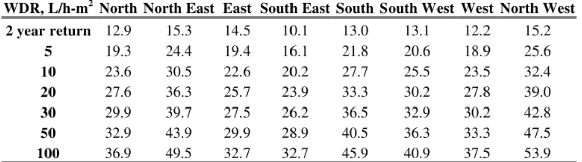
TABLE 6 gives the directional extreme values of WDR and TABLE 7 of DRWP for Philadelphia.
A table of spray rates and DRWP pairs can readily be generated similar to the table listed above by simply referring to the appropriate corridor. The top rows represent the expected DRWP and the columns the expected WDR spray rates. The annual likelihood of occurrence of a pair can be estimated as the product of the return periods, this based on the imperfect assumption of statistical independence (Eq 9).
Likelihood(Direction) = (1/TWDR(Direction)) (1/TDRWP(Direction)) (9)
In-Service Conditions for Wind and Rain
Extreme value analysis gives an estimate of the maximum or extreme loads or events that might possibly occur for a certain probability, generally expressed as the return period. These loads do not represent typical in-service conditions. To obtain typical in-service conditions it was necessary to examine the WDR and DRWP datasets using a different statistical approach.
TABLE 6 ― Table of expected extreme values of WDR for eight directions for Philadelphia, PA.
WDR, L/h-m2 North North East East South East South South West West North West
2 year return 12.9 15.3 14.5 10.1 13.0 13.1 12.2 15.2 5 19.3 24.4 19.4 16.1 21.8 20.6 18.9 25.6 10 23.6 30.5 22.6 20.2 27.7 25.5 23.5 32.4 20 27.6 36.3 25.7 23.9 33.3 30.2 27.8 39.0 30 29.9 39.7 27.5 26.2 36.5 32.9 30.2 42.8 50 32.9 43.9 29.9 28.9 40.5 36.3 33.3 47.5 100 36.9 49.5 32.7 32.7 45.9 40.9 37.5 53.9
The first task was to fit a probability density function (PDF) or statistical distribution to rain events and coincident wind events. The first step in this task was to construct a histogram of wind events by allotting rain events of specific magnitudes into bins. A PDF was then fitted to each of the histograms using a Weibull distribution.
Such types of distributions have been shown to be useful in fitting climate or weather data for engineering purposes [20, 21, 22]. For example, Justus [28] discussed the
applicability of the Weibull distribution for estimating wind frequency distributions especially the advantage of projecting the distribution to other wind speed heights. Much of the reported work on fitting Weibull distributions to wind speed data speed is related
to the estimation of parameters for assessing wind power [29, 30]. The general consensus is that the Weibull distribution is appropriate for modeling wind data [31, 32, 33, 34].
TABLE 7 ― Table of expected extreme values of DRWP for eight directions for Philadelphia, PA.
DRWP, Pa North North East East South East South South West West North West
2 year return 60.4 85.4 84.3 46.3 74.5 53.8 69.5 77.4 5 84.1 128 123 63.9 106 74.1 98.2 127 10 99.9 157 149 75.6 127 87.6 117 160 20 115 184 174 86.8 148 100 136 192 30 124 199 188 93.3 159 108 146 209 50 134 219 206 101 174 117 159 233 100 149 246 229 112 193 129 177 263
In respect to using a Weibull distribution for categorizing rain events, Wilks [35] and Testa [36, 37] have demonstrated the fit of short-term rain data using a Weibull
distribution. Hence, there are useful examples on the use of this type of distribution for categorizing both rain and wind events.
FIGURE 5 shows the cumulative probability function (CDF) for wind speeds and rainfall intensities for Seattle, WA. The CDFs derived from the sample data and the Weibull estimates are shown, as well as the root mean squared error.
Having determined the basic distribution parameters it was then possible to estimate, using the percentage point function, the magnitude of the wind speed for a given
likelihood of occurrence of an event. Common statistics for the two-parameter Weibull distribution are given in TABLE 8 whereas in TABLE 9, the corresponding WDR intensities and DRWPs for various likelihoods of occurrence obtained from the cumulative distribution function are provided.
Given the magnitudes of rainfall intensity and DRWP at various probabilities of occurrence, a table of rainfall and wind speed pairs was then constructed for Philadelphia, as given in TABLE 10. Pairs for the other cities surveyed in this study, Boston, Miami, Minneapolis, and Seattle, are in given in the Appendix, Tables A1 to A4. The values provided in TABLE 10 assume statistical independence between the occurrence of rainfall and the DRWP. However, as previously noted, this assumption is imperfect, and is particularly in doubt in mountainous terrain.
FIGURE 5 – Cumulative distribution functions for rainfall intensity (mm/h) and wind speed (m/s) for Seattle, WA, and corresponding Weibull estimates. The shape and scale parameters as well as the root mean squared error between the actual and assumed distributions are given. The period of record was 26 years.
TABLE 8 – Basic statistics and formulas for the two-parameter Weibull distribution.
Statistic Formula Mean
⎟⎟
⎠
⎞
⎜⎜
⎝
⎛ +
Γ
γ
γ
α
1
Median α 1/γ ) 2 ln( Mode 1 ) 1 1 ( − 1/ γ > γ α γK 1 0Kγ ≤ Standard Deviation 2 1 2 ⎟⎟ ⎠ ⎞ ⎜⎜ ⎝ ⎛ ⎟⎟ ⎠ ⎞ ⎜⎜ ⎝ ⎛ + Γ − ⎟⎟ ⎠ ⎞ ⎜⎜ ⎝ ⎛ + Γ γ γ γ γ αPercent point function α 1/γ )) 1 ln( ( ) (p p G = − −
TABLE 9 ― DRWPs (Pa) and WDR intensities (L/m2-h) for various likelihoods from the Cumulative Distribution Functions. The period of record was 1961-1995.
Location BOS MIA MSP PHL SEA
Cumulative Probability DRWP WDR DRWP WDR DRWP WDR DRWP WDR DRWP WDR 0.5 23 1.44 15 1.69 21 1.21 14 1.23 13 0.93 0.9 71 7.82 55 16.5 47 6.14 48 7.28 38 3.71 0.95 91 11.4 74 27.4 56 8.80 63 10.8 47 5.03 0.99 136 21.1 118 63.4 74 15.9 98 20.6 68 8.25 0.995 155 25.8 138 83.7 82 19.4 114 25.4 77 9.72 1a 492 159 548 1060 190 113 420 171.3 225 41.7 a - 0.99999 probability
Modifying the Loads
This section presents methods for modifying the two basic load parameters, i.e., WDR
and DRWP, to suit specific conditions. Both loads depend on one or two of the basic
input parameters, specifically rainfall intensity and wind speed. Two general classes of modifiers are considered: (i) modifiers for aerodynamic effects, and (ii) those that account for shorter time-averaging periods. It is useful to recall the two basic load-generating Eqs 1 and 5, when reviewing the following sections.
Aerodynamic Effects
Rain Deposition Factor ― The RDF accounts for the aerodynamic effects caused by the
building on the flow field around the building. The flow field is either slowed near the center of the building or accelerated near the edges. As is evident in Eqn 1, the RDF is a
scalar factor in the calculation of WDR. To calculate loads at various points of interest on
the building, the free wind-driven rain, that is, the rain field in absence of a building downstream is multiplied by the appropriate RDF. Straube and Burnett [15] have
TABLE 10 ― Hourly pairs of in-service conditions for wind driven-rain (WDR) and driving rain wind pressure (DRWP) for Philadelphia, PA. The likelihood is an estimate of the cumulative probability that the WDR and DRWP pair will occur.
Cumulative
Probability 0.5 0.9 0.95
Wind speed, m/s 4.68 8.77 10.06
Rainfall, mm/h WDR, l/m2-h DRWP, Pa Likelihood, % WDR, l/m2-h DRWP, Pa Likelihood, % WDR, l/m2-h DRWP, Pa Likelihood, %
0.1 0.12 0.22 14 5.00 0.40 48 9.00 0.46 63 9.50 0.2 0.28 0.43 14 10.00 0.80 48 18.00 0.92 63 19.00 0.3 0.48 0.66 14 15.00 1.24 48 27.00 1.43 63 28.50 0.4 0.73 0.93 14 20.00 1.74 48 36.00 1.99 63 38.00 0.5 1.04 1.24 14 25.00 2.31 48 45.00 2.66 63 47.50 0.6 1.45 1.61 14 30.00 3.01 48 54.00 3.46 63 57.00 0.7 1.99 2.08 14 35.00 3.91 48 63.00 4.48 63 66.50 0.8 2.80 2.75 14 40.00 5.16 48 72.00 5.92 63 76.00 0.9 4.26 3.88 14 45.00 7.28 48 81.00 8.35 63 85.50 0.95 5.80 5.01 14 47.50 9.39 48 85.50 10.78 63 90.25 0.975 7.40 6.14 14 48.75 11.51 48 87.75 13.21 63 92.63 0.99 9.59 7.64 14 49.50 14.31 48 89.10 16.42 63 94.05 0.995 11.31 8.77 14 49.75 16.43 48 89.55 18.86 63 94.53 0.998 13.63 10.27 14 49.90 19.24 48 89.82 22.08 63 94.81 1 48.64 30.81 14 50.00 57.74 48 90.00 66.27 63 95.00
The likelihood of X given Y is the likelihood of X. The likelihood of X and Y is product of the likelihoods. Each rainfall intensity wind speed pair produces a corresponding WDR and DRWP pair.
Wind Speed Correction ― The variation in the mean wind speed with height is most
commonly approximated by a power law representation [38]. The generalized equation (Eq 10) for the wind factor, ft, is used to adjust the wind speed from the height at the measurement site, Hmet, such as a meteorological station to the height of interest at a specific building, h. Typical exponents, a, and boundary layer thicknesses δ are given in TABLE 11. a amet met met t h H f ⎟ ⎠ ⎞ ⎜ ⎝ ⎛ ⎟⎟ ⎠ ⎞ ⎜⎜ ⎝ ⎛ = δ δ (10)
TABLE 11 ― Parameters for standard terrain classifications [38].
Terrain a δ Description
1 0.33 400 Large city centers
2 0.22 370 Urban and sub urban areas, wooded areas etc. 3 0.14 270 Open terrain with scattered obstructions 4 0.10 210 Flat unobstructed areas
The effect of wind on WDR is scalar. To modify the loads for the effect of height and
terrain the wind speed multiply by the appropriate wind terrain factor, ft. The effect of wind on DRWP is also scalar. To modify the loads for the effect of height and terrain the
wind speed multiply by the square of the appropriate wind terrain factor, ft.
Ro’s work [33] suggests that assuming a Weibull distribution for wind speeds is robust over different averaging periods for wind speed datasets collected over long periods of time. For shorter study periods, e.g., five days in Ro’s study, wind speed data does not seem to fit a Weibull distribution.
Wind Speed ― For events having durations shorter than one hour the rainfall intensities
may be greater and the wind speeds higher. Factors, fs and fp, that relate wind speed and wind pressure, respectively, for converting hourly wind speeds to averages over 1, 3, 5, 10, and 15 minutes have been extracted the ASCE Standard, Minimum Design Loads for Buildings [39].
Time Averaging
The wind speed and wind pressure adjustment factors are given in TABLE 12. To increase the WDR and DRWP loads simply multiply the loads by the appropriate speed or pressure factor.
Averaging Time 15 minutes 10 minutes 5 minutes 3 minutes 1 minute
Factor on speed,fs 1.04 1.07 1.11 1.14 1.25
Factor on pressure, fp 1.08 1.14 1.23 1.30 1.56
Rainfall Intensity ― The factor for converting hourly rain intensities falling vertically
onto a level surface to shorter averaging periods, rt, has been suggested by Choi [40] and is provided in Eq 11. 42 . 0 3600 ⎟ ⎠ ⎞ ⎜ ⎝ ⎛ = t r rt h (11)
where t, time, is in seconds.
As indicated by Eq1 WDR load is not only a scalar product of horizontal rainfall intensity and wind speed but also depends on the DRF. The relationship between the
DRF and rainfall intensity is nonlinear, depending on the raindrop size and terminal velocity of the raindrops. Consequently it is not possible to derive a single modifier for a given averaging time given that the modifier depends on the averaging period and rainfall intensity.
FIGURE 6 shows values for DRF60 calculated for various hourly intensities. FIGURE 7 shows the ratio of DRTt to DRF60 for various averaging times. This ratio is the driving-rain factor modifier, fdrf. Therefore to modify the DRF for a shorter averaging period at a
given hourly rainfall intensity fdrf can be read off directly from FIGURE 7 for desired averaging period given rh. DRF60 is read off FIGURE 6. The product of DRF60 and fdrf
yields the appropriate DRF. Alternatively the DRF can be calculated directly from Eqs
2-4 using a modified intensity for shorter averaging periods, rt, or read off from FIGURE 6 directly given, rt.
For example, suppose the 1 in 2 (the 50 % or median value) 15 minute WDR intensity is of interest. The median value for rainfall intensity in Philadelphia is 1.04 mm/h. The 15 minute value, rt, is 1.04 * (3600/900)0.42 = 1.04 * 1.79 1.86 mm/h. The DRF from Eqs 2-4 or FIGURE 6 is 0.226 s/m. Alternatively if using the unmodified median value, 1.04 mm/h, DRF60 is 0.25 (from FIGURE 6) and from FIGURE 7 fdrf is 0.89. The product of
terms is 0.223 s/m, as before. Examples of frain and fdrf are shown in for several common measures of the Weibull distribution.
The most conservative assumption is to assume that the DRF modifier, fdrf, is 1. This is the recommended approach for modifying extreme loads. For in-service conditions assuming a value of 1 for the DRF modifier, fdrf, is also a conservative assumption.
FIGURE 6 ― Chart for estimating the DRF60 for hourly average rainfall, mm/h.
FIGURE 7 ― Chart for estimating the driving-rain factor modifier, fdrf, for shorter veraging periods using hourly average rainfall, rh, mm/h as input.
TABLE 14 ― Rain and driving rain factor, DRF for shorter averaging times for in-service conditions for Philadelphia, PA.
Averaging Time rh 15 minutes 10 minutes 5 minutes 3 minutes 1 minute
Factor on rain, frain n/a 1.79 2.12 2.84 3.52 5.58
0.09 0.88 0.85 0.80 0.76 0.69 DRF modifier, mode, fdrf 0.74 0.90 0.87 0.83 0.80 0.74 DRF modifier, mean, fdrf 1.04 0.89 0.87 0.82 0.79 0.73 DRF modifier, median, fdrf 4.26 0.91 0.88 0.84 0.81 0.76 DRF modifier, 90th %, fdrf
A Methodology for Determining the Magnitude and Likelihood of Wind-Driven Rain Loads on Building Façades
The methodology outlined in this paper is to be used to determine the wind driven-rain and driving rain wind pressure loads for North American locations and the corresponding probability of occurrence. This method can be applied to most locations; however caution should be exercised when it is suspected that the qualifying assumptions may not hold, as might be the case for mountainous terrain or coastal regions. In such regions a more detailed analysis is required. The general process is as follows:
Step 1. Obtain historical climate data for the location of interest. A minimum record
length of ten years is suggested. A maximum averaging time of 1 hour is also
recommended. The required data fields are: rainfall6, concurrent wind speed and wind direction data. Useful but optional fields are: temperature (to calculate air density), atmospheric moisture (wet bulb, dew point or RH to calculate air density) and station pressure (to calculate air density). The measurement station should also provide basic information such as longitude, latitude, and elevation.
Step 2. From the historical data produce a new dataset containing hourly rainfall,
wind speed and direction, wind driven-rain, and driving rain wind pressure (Eqs 1 and 5).
Step 3. If the qualifying assumption of statistical independence between rainfall
intensity and wind speed holds, produce two subsets of the annual maximum WDR and DRWP loads. If the location is in a mixed climate then perform an EVA. Otherwise, assuming a TYPE I GEV, compute the expected values for given return periods using Eqs 6 and 7 for both WDR and DRWP, from the sample set statistics, (i.e., sample mean and unbiased standard deviation).
Step 4. For each pair of WDR and DRWP estimate the likelihood of occurrence. The
probability of a certain WDR load given a certain DRWP load is simply the probability of the WDR and vice versa, assuming statistical independence. The probability of both events occurring is the product of both probabilities. Using this approach a table of likelihoods for various pairs of extreme WDR and DRWP loads can be produced.
Step 5. If directional information is required, repeat Steps 3 and 4 with the exception
that the dataset be broken into individual rain corridors (minimum of eight corridors). Steps 3 and 4 are then repeated for each corridor.
6
Rainfall data are required. If precipitation data are available, rainfall should be separated from solid precipitation. A present weather observation is useful in this respect. Ideally rain gauge data, such as tipping bucket data, would be best. Radar and satellite data are also available; however, the assessment of the reliability of these data was beyond the scope of this study.
Step 6. For in-service loads (i.e., nonextreme), fit rainfall intensity and wind speed to
a two-parameter Weibull distribution. The distribution parameters can then be estimated using many different methods. One of the easiest methods is to linearize the cumulative distribution function and regress on the resultant dataset to estimate the distribution parameters.
Step 7. Once the distribution parameters have been estimated, for in-service loads use
the percent point function to estimate the likelihood of occurrence of certain rainfall intensities or wind speeds. The percent point function, also commonly referred to as the inverse distribution function, is the inverse of the cumulative distribution function.
Step 8. For in-service loads (nonextreme), calculate for each pair of rainfall intensity
and wind speed, the WDR and DRWP load. For each pair of WDR and DRWP estimate
the likelihood of occurrence. The probability of a certain WDR given a certain DRWP
load is simply the probability of the WDR and vice versa, assuming statistical
independence. The probability of both events occurring is the product of both
probabilities. Using this approach a table of likelihoods for various pairs of in-service WDR and DRWP loads can be produced.
Step 9. If directional information on in-service loads is required the dataset should be
broken into individual rain corridors, a minimum of eight. Steps 6, 7, and 8 are then repeated for each corridor.
Step 10. Modify the loads to suit particular circumstances using the appropriate
modifying factors.
Summary and Recommendations
The work described here primarily relates to water penetration and water leakage of building façades. The objectives of the work were to: (i) investigate the basis for the spray rates prescribed in various standards; (ii) relate the water spray rates and applied pressure differences applied to test specimens to the likelihood of occurrence, and (iii) develop a methodology for determining spray rates and applied pressure differences for a given likelihood of occurrence. Test protocols can be developed for specific locations or a standard test protocol can be related to specific locations using the methodology.
Five cities in the United States were examined: Boston, Miami, Minneapolis-St. Paul, Philadelphia, and Seattle. Given the small number of stations examined, five out of the several hundred in the SAMSON and HUSWO datasets, any conclusions regarding the results must be guarded. Generally there were no oddities in the probably distributions derived from the data with one exception. The extreme value data for Miami clearly shows that there are two sets of data – “normal” extremes and those due to hurricanes. This is typical of mixed climates where a longer period of record might be required for convergence of GEV Type I distributions. The traditional approach is to create a
composite chart categorizing the events according to the underlying synoptic phenomena. There are other approaches, however, and a more detailed study of mixed climates is warranted.
The 3.4 L/min-m2 (204 L/h-m2), the base spray rate used in the ASTM E331 and E547 methods, is high for most cases especially for hour-long durations. In all the locations included in this evaluation, this spray rate exceeds typical annual maximum values for WDR, never mind typical in-service values for WDR. However, if shorter duration episodes are considered, e.g., 15 minutes or shorter, the 204 L/h-m2 mark may
be reasonable. Miami was exceptional with regard to the distribution of annual maximum WDR values. In Miami, where hurricanes sometimes occur, there seems to be a
reasonable chance, 1 in 30, of that the maximum annual WDR value will be equivalent to 3.4L/min-m2 with a duration of an hour. The study also indicates that the extreme
driving-rain wind pressures in the order of 500 Pa can occur. Thus the 700 Pa level found in some protocols is clearly justified. What is not clear, however, is the likelihood of both extreme driving-rain and extreme driving-rain wind pressure occurring simultaneously. In Miami, FL, the higher values for WDR do not necessarily occur during the windiest events. The most extreme hourly wind-driven rain event in the record set, 378 L/h-m2, occurred with an hourly wind speed of 92.7 m/s just below the hurricane storm threshold.
The next most extreme hourly wind-driven rain event in the record set, 221 L/h-m2, occurred with an hourly wind speed of 11.2 m/s well below the tropical storm threshold.
Thus the combined spray rates and pressure differences used in most protocols and
standards appear to be a bit higher than warranted given that the probability of occurrence for these events is low; they occur very rarely, even during unusually strong storms. Their probability of occurrence is even lower when the dataset used to determine probability incorporates all in-service rain events (not just the more extreme events).
Despite the limited number of locations analyzed in this study, the observations made for four of the five locations suggest that the methodology is probably applicable to most locations within the conterminous United States. Analysing wind-driven rain data in this manner is useful for understanding the variances in the rain loading on building façades in terms of both extreme events and of more typical in-service conditions. The
methodology builds upon the work previously carried out by Underwood and others. It could be used as the basis for a comprehensive wind-driven rain atlas and serve as a basis for standards and codes development.
Although our investigations suggest that the methodology can be applied to most locations, caution should be exercised when it is suspected that qualifying assumptions may not apply, as might be the case for mountainous terrain or coastal regions. In such regions a more detailed analysis is probably required.
In conclusion, a methodology that attempts to derive appropriate testing levels on a statistical analysis of climatic or weather-based related to likelihoods of occurrence has been described. The limitations of the study are: (i) the small number of locations used in the analysis; (ii) the lack of analysis of events of duration less than one hour; (iii) the assumption of statistical independence between wind speed and rainfall intensity, and (iv) the need for a more detailed analysis of mixed climates. The first limitation can be
remedied through continued work. The other limitations cannot be solved until finer grained datasets become available.
References
[1] Blocken, B. and Carmeliet, J., “A Review of Wind-Driven Rain Research in Building Science,” Journal of Wind Engineering and Industrial Aerodynamics,
Vol. 92(13), 2004, pp. 1079-1130.
[2] Hoppestad, S., Slagregn i Norge (in Norwegian), Norwegian Building Research Institute, rapport Nr. 13, Oslo, 1955.
[3] Lacy, R.E., Climate and Building in Britain, Building Research Establishment Report, London, UK: Department of the Environment, Her Majesty’s Stationary, Office, 1977. ISB/SN/CDN 0026-1149
[4] Lacy, R.E. and Shellard, H.C., “An index of driving rain” Meteorological Magazine, Vol. 91, 1962, pp.177-184. ISSN 0144-8536
[5] Lacy, R.E., “An index of exposure to driving rain”, Building Research Station Digest 127, Garston, UK, 1971.
[6] Underwood, S.J. and Meentemeyer, V., “Climatology of wind-driven rain for the contiguous United States for the period 1971 to 1995,” Physical Geography, Vol. 19(6), 1998, pp. 445-462.
[7] Leslie, N.P., “Laboratory Evaluation of Residential Window Installation Methods in Stucco Wall Assemblies,” ASHRAE Transactions, Vol. 113, Part 1, 2007, pp. 296-305. ISSN 0001-2505 1088-8586 (CD-ROM version)
[8] Teasdale-St-Hilaire, A. and Derome, D., “Methodology and Application of Simulated Wind-Driven Rain Infiltration in Building Envelope Experimental Testing,”
ASHRAE Transactions, Vol. 112, Part 2, 2006, pp. 656–670. ISSN 0001-2505 1088-8586 (CD-ROM version)
[9] Lacasse, M.A. "Durability and performance of building envelopes," BSI 2003 Proceedings (October, 2003), pp. 1-6 (NRCC-46888)
[10] Cornick, S.M. and Lacasse, M.A. "A Review of Climate Loads Relevant to
Assessing the Watertightness Performance of Walls, Windows and Wall-Window Interfaces," Journal of ASTM International, 2(10), Nov/Dec., 2005, pp. 1-16. [11] Lacasse, M.A., O'Connor, T., Nunes, S.C., Beaulieu, P., Report from Task 6 of
MEWS Project: Experimental Assessment of Water Penetration and Entry into Wood-Frame Wall Specimens - Final Report, Research Report, Institute for
Research in Construction, National Research Council Canada, (IRC-RR-133), 2003. [12] CSA, Canadian Supplement to AAMA/WDMA/CSA 101/I.S.2/A440-05,
Standard/Specification for windows, doors, and unit skylights Canadian Standards
Association, Mississauga, Ontario, Canada, 128 p.
[13] National Oceanic and Atmospheric Administration, Solar and Meteorological Surface Observational Network 1961-1990 Version 1.0, September 1993. National Climatic Data Center Federal Building151 Patton Avenue Asheville NC 28801-5001.
[14] National Oceanic and Atmospheric Administration, Hourly United States Weather Observations, 1990-1995, October 1997. National Climatic Data Center Federal Building151 Patton Avenue Asheville NC 28801-5001.
[15] Straube, J.F. and Burnett, E.F.P., Building Science for Building Enclosures, Chapter 12, Building Science Press, Westford, MA, 2005, 549 p.
[16] Dingle, A.N. and Lee, Y., “Terminal fall speeds of raindrops,” Journal of Applied Meteorology, Vol. 11, August 1972, pp. 877-879.
[17] Best, A.C., “The size distribution of raindrops,” Quarterly Journal of Royal Meteorological Society, Vol. 76, 1950, pp. 16-36.
[18] Choi, E.C.C., “Wind-Driven Rain and Driving Rain Coefficient During Thunderstorms and Non-Thunderstorms,” Journal of Wind Engineering and Industrial Aerodynamics, Vol. 89, 2001, pp. 293–308.
[19] Blocken, B. and Carmeliet, J., "On the Validity of the Cosine Projection in Wind-Driven Rain Calculations on Buildings," Building and Environment, Vol. 41(9), 2006, pp. 1182-1189.
[20] Ang, A.H.S., and Tang, W.H., Probability Concepts in Engineering Planning and Design – Vol. 1, Basic Principles, John Wiley & Sons, NY, (2001), 424 p.
[21] Bras, R.L., Hydrology: An Introduction to Hydrologic Science, Addison Wesley,
Boston, MA, 1990, 643 p.
[22] Hahn, G.J. and Shapiro, S.S., Statistical Models in Engineering, John Wiley & Sons,
New York, 1968, 355 p.
[23] Palutikof, J.P., Bradcock, B.B., Lister, D.H., and Adcock, S.T., "A review of
methods to calculate extreme wind speeds," Meteorological Applications, Vol. 6(2) (1999), pp. 119-132. ISSN 1469-8080
[24] Cook, N.J., The Designer’s Guide to Wind Loading of Building Structures. Part 1: Background, Damage Survey, Wind Data and Structural Classification. Building Research Establishment, Garston, and Butterworths, London, 1985, 371 pp. [25] Cook, N.J., Harris, R.I. and Whiting, R., "Extreme wind speeds in mixed climates
revisited," Journal of Wind Engineering and Industrial Aerodynamics, Vol. 91(3), 2003, pp. 403-422.
[26] Cook, N.J., "Confidence limits for extreme wind speeds in mixed climates." Journal of Wind Engineering and Industrial Aerodynamics, Vol. 92(1), 2004, pp. 41-51. [27] Gomes, L. and Vickery, B.J., "Extreme wind speeds in mixed wind climates,"
Journal of Wind Engineering and Industrial Aerodynamics, Vol. 2(4), 1978, pp. 331-344.
[28] Justus, C.G., Hargraves, W.R., Mikhail, A. and Graber, D."Methods for Estimating Wind Speed Frequency Distributions," Journal of Applied Meteorology, 17(3), 1978, pp. 350-353.
[29] Stevens, M.J.M., and Smulders, P.T., "Estimation of the parameters of the Weibull wind speed distribution for wind energy utilization purposes," Wind Engineering, Vol. 3(2), 1979, pp. 132-145.
[30] Seguro, J.V. and Lambert ,T.W., "Modern estimation of the parameters of the Weibull wind speed distribution for wind energy analysis," Journal of Wind Engineering and Industrial Aerodynamics, Vol. 85(1), 2000, pp. 75-84.
[31] Tuller, S.E. and Brett, A.C., "The Characteristics of Wind Velocity that Favor the Fitting of a Weibull Distribution in Wind Speed Analysis," Journal of Applied Meteorology, Vol. 23(1), 1984, pp. 124-134. ISSN 0894-8763 1520-0450 [32] Deaves, D.M. and Lines, I.G., "On the fitting of low mean wind speed data to the
Weibull distribution." Journal of Wind Engineering and Industrial Aerodynamics, Vol. 66(3), 1997, pp. 169-178.
[33] Ro, K.S. and Hunt, P.G., "Characteristic Wind Speed Distributions and Reliability of the Logarithmic Wind Profile," Journal of Environmental Engineering, Vol. 133(3), 2007, pp. 313-318.
[34] Celik, A.N., "Weibull representative compressed wind speed data for energy and performance calculations of wind energy systems," Energy Conversion and Management, Vol. 44(19), 2003, pp. 3057-3072.
[35] Wilks, D.S. "Rainfall intensity, the Weibull distribution, and estimation of daily surface runoff," Journal of Applied Meteorology, Vol. 28(1), 1989, pp. 52-58.