AUTOMATIC CLASSIFICATION OF SEISMIC
DETECTIONS FROM LARGE-APERTURE SEISMIC ARRAYS by
SEYMOUR SHLIEN
B.Sc. McGill University (1968)
SUBMITTED IN PARTIAL FULFILLMENT
OF THE REQUIREMENTS FOR THE DEGREE OF DOCTOR OF SCIENCE
at the
MASSACHUSETTS INSTITUTE OF- TECHNOLOGY June 1971 ( ,97 i
Signature of Author .,.,/. .- . . .i .- -.
Department of 'arth and Planetary Sciences
Certif ied by . . . . .'y' 0- 0 .0 . Thesis Supervisor
Accepted bi-.- . -.' w., g. ..
Chairman, Depa tmental Committee pn Graduate Students
Z sM
S
AUTOMATIC CLASSIFICATION OF SEISMIC DETECTIONS FROM LARGE APERTURE SEISMIC ARRAYS
by
Seymour Shlien
Submitted to the Department of Earth and Planetary Sciences on May 5, 1972
in partial fulfillment of the requirements for the degree of Doctor of Science
The large-aperture seismic arrays in Montana (LASA) and Norway (NORSAR) make on-line signal processing a necessity
if these arrays are to be used at their full capability. Using the outputs of the detection processors of the
re-spective arrays, the feasibility of automatic classification of seismic signals into the various body phases P, PKP, PcP, ScP, SKP, PP, PKKP and P'P' was confirmed. It was shown how these later phases can be used to advantage in improving the location capability using the combination of the two arrays.
One of the byproducts of this study was an estimation of the detection and location capabilities of the arrays.
It was estimated that LASA detects more than 50 real seismic signals a day, of which less than 10% are due to later phases. LASA's detection capability extends almost one body wave
magnitude below ERL's capability based on reported epicenters. The discrimination between very weak seismic signals and
false alarms due to spurious noise was found difficult on the basis of only the detection logs.
Only a little more than 8 earthquakes a day were found common between LASA and NORSAR arrays. It is expected that this number will increase with the improved signal processing that the two arrays recently implemented.
Thesis Supervisor: M.N. Toksoz Title: Professor of Geophysics
11
ACKNOWLEDGMENTS
I am indebted to Nafi Taks*z, who was my advisor through-out my four years of graduate study at M.I.T. He had ori-ginally suggested this problem and had given me constant en-couragement.
I am especially grateful to Dr. Richard Lacoss, who had sacrificed a lot of his time in following my work. His
sympathy for my frustrations and excellent sense of humor are deeply appreciated.
Thanks go to Dr. Charles Felix (IBM), Dr. Richard Lacoss (Lincoln Laboratory), Prof. Seymour Papert (Artificial
In-telligence Group) and Prof. Michael Godfrey (Civil Engineering) whose discussions helped me get started. Also I would like to thank Mr. Larry Lande and Mr. Russell Needham, who had taught me to read seismograms.
In addition, I would like to thank Dr. William Dean of IBM, Mr. Simon Sarmiento (IBM), Mr. Albert Taylor (MIT), Mr. Lawrence Sargent (Lincoln Laboratory) and Miss Mary O'Brien
(Lincoln Laboratory) who had helped procure the detection logs and summary bulletins.
Thanks go to Mr. Jerry Moore (IBM), Mr. Tom Murray, Mr. Philip Fleck and Miss Leslie Turek of Lincoln Laboratories, Mr. Richard Steinberg and Mrs. Jean Bow (Information Processing Center) for programming assistance.
Prof. Theodore Young (Pattern Recognition Group) had shown much interest and made many valuable suggestions in the final stages of this work.
I would also like to acknowledge the helpful discussions I had with Dr. Jack Capon and Mr. Robert Sheppard of Lincoln Laboratory and Mr. Guy Kuster and Mr. Norman Brenner (MIT).
I was supported by a Lincoln Laboratory Fellowship
1970-1971 and by a Chevron Oil Research Fellowship 1971-1972. This project was supported by the Advanced Research Project Agency and monitored by the Air Force Office of Scientific Research under Contract No. F44620-71-C-0049.
iv TABLE OF CONTENTS Page Abstract 1 Acknowledgements ii Table of Contents iv List of Figures vi List of Tables X 1. Introduction 1
2. LASA and NORSAR Capablities 8
2.1 Introduction 8
2.2 SAAC signal processor 8
2.3 Detection capability of LASA and NORSAR 12 2.4 Location capability of LASA and NORSAR 18 2.5 Depth and magnitude estimation 19
2.6 Conclusions 20
3. Pattern Recognition as Ap'lied to Seismic 23 Array Problems
3.1 Introduction 23
3.2 Pattern recognition 25
3.3 Training set 31..
3.4 Summary 37
4. Classification of Detections Using One Array 38
4.1 Introduction 38
4.4 Conclusions 56 5. The vo Array phase Identifier 59
5.1 Introduction 59
5.2 Two-array phase identifier 60 5.3 Locating earthquakes with two arrays 68
5.4 Conclusions 72
6. Conclusions 73
References 77
Appendices 80
A Criterion for Matching Predicted Signals 80 to the Detection Log
B Distance and Azimuth Resolution of a Large- 83 Aperture Seismic Array
B.l Introduction 83
B.2 Distance resolution 83
B.3 Azimuth resolution 85
C Improved. Discrimination -of. Signals from 88 False Alarms
D Shuffling a Detection Log 91
E Numerical Evaluation of li for the Single 93 Array Phase Identifier
F Spherical Surface Transformation 96
vi
LIST OF FIGURES
1. Ray paths of the different seismic phases (Richter, 1958).
2. LASA seismograms of large magnitude ( mb o 5.5)
earthquakes at various distances (A) from LASA. The gain factor was adjusted for the best repro-duction. The phases from the distant events have a low signal-to-noise ratio. The seismograms have been sampled 20 times a second. The bottom trace indicates two-second marks.
3. (Upper) Block diagram of LASA signal processor.
(Lower) Block diagram of LASA's Detection Processor. 4. P & PKP phase locations of LASA beams (high
resolu-tion partiresolu-tion) as given by SAAC and plotted on an equidistant projection centered at LASA. 5. Number of earthquakes reported by ERL (white) &
number of earthquakes reported by ERL and detected by LASA (black) as a function of distance.
6. Number of earthquakes reported by ERL (white) & number of earthquaes reported by ERL and detected by NORSAR (black) as a function of distance.
7. Percentage of ERL earthquakes less than 80 degrees from the respective arrays that were detected as a function of body wave magnitude.
8. Percentage of ERL earthquakes greater than 80 degrees distance from the respective arrrays that were de-tected as a function of body wave magnitude.
9. Number of earthquakes reported by ERL (white) and number of earthquakes reported by LASA (black) as a function of distance.
10. Correlation of LASA body wave magnitude versus ERL body wave magnitude for the same events.
11. Frequency magnitude distribution of earthquakes less than 95 degrees from their respective arrays deter-mined from LASA and NORSAR bulletins and ERL catalog. 12. Time interval between later and first arrival in
seconds measured at LASA versus ERL determined epicenter distance from LASA for PcP, ScP, PP-P PP-PKP and SKP phases.
13. Time interval between later and first arrival mea-sured at LASA in seconds versus ERL determined distance of epicenter from LASA for P'P', PKKP-P, and PKKP-PKP phases.
14. Histograms of distance and azimuth errors of epicenter determinations for LASA and NORSAR Summary Bulletins. 15. Maximum MSTA in a detection group versus summary
bulletin reported amplitude in millimicrons for LASA and NORSAR. Scatter was reduced by averaging MSTA over 0.1 millimicron units.
viii
16. MSTA distribution of all detections and of only false alarms in the LASA and NORSAR detection log.
17. False alarm probability given MSTA for LASA and NORSAR. 18. Cumulative probability distribution function of the
maximum MSTA of detection groups matched to reported signals in the LASA and NORSAR Summary Bulletins. 19. Cumulative number of reported events in summary
bulletin, estimated cumulative number of false
alarms, and estimated cumulative number of signals, versus MSTA for LASA and NORSAR.
20. Travel time interval between first arrival and later phase versus the inverse phase velocity of the later phase.
21. Empirical frequency distribution of parameters Sl,
S2, and S3 of the LASA single array phase identifier determined for correctly identified detection pairs and random detection pairs.
22. Log MSTA ratio of fist arrival to later phase for various phases.
23. LASA (L), NORSAR (N), and chosen (L) beam locations plotted with travel time interval curve for various phase combinations. Actual epicenter is at X.
B-l. Distance and azimuth of epicenters triggering specific LASA high resolution beams.
E-l. Cumulative probability distribution function of
LASA's MSTA for all beams (left) and for only aseismic beams (right).
F-l. Partial derivative of distance of a point from NORSAR with respect to distance from LASA as a
function of LASA distance and azimuth. Grid spacing is in 10 degree intervals and the origin is at (0,0).
x
LIST OF TABLES
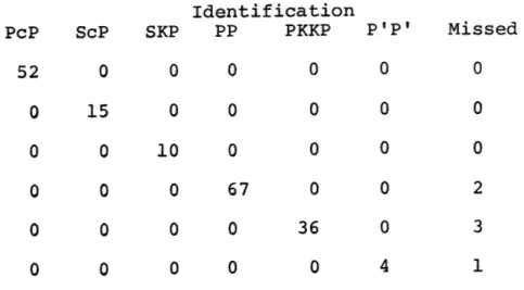
1. Confusion matrix for single array phase identifier. 2. Distribution of correctly and incorrectly classified
training phase pairs determined from the two-array phase identifier.
E-1 Approximations to the decsion parameters of the single array phase identifier.
Introduction
The Large Aperture Seismic Array in Montana (LASA) has made it possible to detect and locate earthquakes in real time over at least half the surface of the earth.
Through the on-line processing of signals from 525 seismometers spread over an aperture of 200 kilometers, noise has been
reduced to low enough levels to multiply the number of detectable earthquakes by at least a factor of two. The Seismic Array Analysis Center (SAAC) at Washington reports about 30 earthquakes on an average day. These earthquakes are located within several hundred kilometers within
several hours after they occurred.
LASA is generating a very large data base by which one can eventually map the interior of the earth to finer detail. This thesis is mainly devoted to studying the contents of the detection log. The detection log is the direct output of the Detection Processor (DP) which attempts to flag every signal arriving at LASA. Many of the
de-tections are not signals but false alarms due to the noise level suddenly increasing. The signals consist of mainly seven different body wave phases. If these detections could be automatically classified, the load of the analyst could be reduced considerably in the preparation of earthquake reports.
Most of the signals detected by LASA are the first arrivals namely P or PKP depending on the distance of the earthquake from the array. In about 10 percent of the cases a later phase such as PcP, ScP, SKP, PP, PKKP or P'P' is also detected. Later phases are caused by re-flections of the seismic signal off the earth's core or free surface. (See Figure 1.) These later phases are both a nuisance and a boon. If a later phase is mistaken as a
P phase then a fictitious earthquake would be reported. On the other hand later phases permit one to get a better estimate of the earthquake's epicenter and may be a decid-ing factor in determindecid-ing whether a detection is real or not. A statistical pattern recognition technique will be developed to classify these detections either using a single array, LASA, or using LASA in conjunction with the Nor-wegian Seismic Array (NORSAR) which went into full operation
in March 1971.
seismograms are shown in Figure 2. Because of this, it is not feasible to incorporate a standard waveform, and the pattern recognition scheme will probably not perform as well as an analyst who has all available information. Nevertheless, the automatic classification scheme will
save the analyst a considerable amount of time and standar-dize the identifications. Eventually an analyst may be necessary to only verify the output of the automatic phase identifier and resolve any conflicting phase identification.
One of the byproducts of this study will be an es-timate of the capabilities of NORSAR and LASA. Eses-timates of the detection and location capabilities are needed for
the automatic phase identifier. Since the estimates ob-tained here are based upon pre-processed data, they will highly reflect the quality of the initial signal processing
and will not be the maximum capabilities of the arrays. This became very evident after this analysis was performed when LASA and NORSAR upgraded their signal processing.
In this study, we had a very small standard data base. Very few of the detections could be identified by an
outside source. It was necessary to rely very heavily on the earthquake catalog distributed by the Environmental
Research Laboratory (ERL) to identify some of the detections. Since the ERL catalog only reports a fraction of the world earthquakes, there was no way of ascertaining that a
specific detection is a false alarm due to spurious noise. Furthermore for many cases it was very difficult to
positively identify a detection using the ERL catalog. There was always an uncertainty whether a predicted phase was properly matched to the detection. For instance it is conceivable that the signal was too small to be detected by LASA and what was observed was either spurious noise or some other signal from a different earthquake. Since the set of pre-identified detections (which we shall later call the training set) was used both to develop and evaluate
th& performance of the automatic phase identifier, some of
the analysis was a little subjective. There was unfortunately little choice in this matter since only three months of
data was available.
The effects of very deep earthquakes were completely ignored in this study. Because 90 percent of earthquakes are relatively shallow and depth effects are complicatedly
related to the phase identification and epicenter determination, they were not incorporated into the phase identifier.
such as pP from the seismic coda without seeing the actual waveforms. For earthquakes shallower than 100 kilometers, the travel time corrections were usually less than thirty seconds and could easily be neglected.
Except for the Seventh IBM Technical Report (1970) there was nothing published on the phase identification problem. No elaborate evaluation on the performance of their scheme has been reported yet.
The remaining part of the thesis is divided into five chapters. In Chapter 2, the SAAC signal processing is described and the capabilities of the arrays are de-termined. The first section describes how the detection log is generated at LASA from the raw signals coming into the 525 seismometers. The beam partitions used by the detection processor is discussed. Off-line processing
to generate the summary bulletins is very briefly described. In the next section the detection capability of the arrays is estimated as a function of distance and magnitude on the basis of the summary bulletins and the detection log using the ERL epicenter determinations as an outside
standard. Since LASA detects many more earthquakes than are listed in any earthquake catalog we had to resort to fre-quency-magnitude distributions to infer the lower magnitude limit of LASA's detection capabilities. The second half
6
of this section describes the location capability of the arrays and the factors that determine this capability.
In Chapter 3 the theoretical framework necessary to understand how the automatic phase identifier works is described. A model of decision making is discussed and the concept of a training set is introduced. The statis-tical pattern recognition technique is described in the next section and examples are given to relate this method to
the problem of distinguishing false alarms from signals and classifying phases. Bayes rule and the maximum likelihood test is briefly reviewed. "A priori, a posteriori proba-bilities", "observation space" and "performance" are defined. An alternative rule which uses the concept of distance is introduced. The distance rule is equivalent to the maximum likelihood test if the decision parameters have an error which is normally distributed.
In Chapter 4 the automatic phase identifier which uses a single array is described. Distributions of the decision parameters are determined and approximated. The programming of the automatic phase identifier is discussed and the
performance of the phase identifier is determined from the LASA detection log.
Chapter 5 describes the two array phase identifiers. Much more information is available from the combination of LASA and NORSAR detection logs so that 50 different
determined, the programming is described and the performance of the identifier is evaluated. A method of improving
the epicenter determined from the two arrays when later arrivals are found is described.
In the final chapter results of this study are summar-ized and conclusions are drawn.
Throughout this thesis an attempt was made to put all the details and mathematics into the appendices. This was done to make the text more readable.
The data analyzed in this thesis was confined to the time period May, 1971, to August, 1971.
Chapter 2
LASA and NORSAR Capabilities
2.1 Introduction
In this chapter we discuss the present LASA signal pro-cessors, their capabilities ,and limitations. We start with
the detection of seismic signals, and follow this by an
esti-mation of detection capabilities of LASA and NORSAR as a func-tion of distance and magnitude, in Secfunc-tion 2.3. The location errors are determined in Section 2.4, and in Section 2.5 we discuss the problems of location errors and magnitude esti-mation.
2.2 SAAC Signal Processor
The signal processing described here is basically that of LASA which was designed and developed by IBM and which went in full operation as of April 1969. The details of the present signal processor are described in the IBM final report (1972).
The processing of the seismic signals by LASA can be se-parated into three steps:(l) detection processing (2) event processing and (3) verification. A block diagram is shown in Figure 3. Since the input of the automatic classifier is the output of the Detection Processor the first step is
described in a fair amount of detail while the other steps are dealt with briefly.
tion of the earthquake and the phase type of the signal. If the output of the individual sensors of the LASA could be
com-bined to screen out all the signals except that coming with
the specific velocity and from the specific direction, the Signal-to-Noise-Ratio (SNR) may be enhanced considerably. The
first step of the Detection Processor (Figure 3) is to generate in real tine a set of 600 presteered beans with different
velocities and azimuths. The beams are formed by delaying and summing the signals of the individual sensors. Let S (t) be the amplitude of the signal at the ith sensor positioned at x. Let v be the velocity vector corresponding to beam m.
m
Then the delay tines tm,i for the sensor i and beam m is given by:
t .=v -x./|v 2(2 )
m,i m 2 (2.1)
The beam b M(t) is forned from the individual sensors using
N
b M(t) =S (t - t Mm) (2.2)
where N is the total number of sensors used by the beam gener-ator. The resolution of the beam Ap in inverse velocity
space is proportional to T/A, where T is the period of the signal and A is the aperture of the array. On account of the configuration of LASA sidelobes are very considerable. The
biggest sidelobe is only 5 db below the main lobe (IBM Final
Report, 1972).
The 600 beams can be separated into two overlapping par-titions of 300 beams each. The first partition which has been in operation since April, 1969, is the set of high resolution beams. Because these beams are narrow, a very large number
of beams are needed to cover all possible areas of velocity space from which one can expect the seismic signal. For eco-nomic reasons only 300 of these narrow beams are conputed. These beams were pointed towards the seismic regions and areas of interest to nonitor nuclear explosions. A plot of these beans on a world map is shown in Figure 4 for the P and PKP phases.
It is evident that the fine beam pattern leaves many gaps in the signal space, in particular for some of the later
phases such as PP. If a seismic signal cones from an area
where there is no beam coverage it would be missed by the de-tection processor if it is a weak signal. However, if the signal is very strong it will leak into a sidelobe of a beam which is pointed very far from the actual signal source. Since this was found to be undesirable, another beam partition con-sisting of low resolution beams was added to the Detection Processor in January, 1972. The second beam partition covers all the seismic signal space, but has much less resolution. Similarly, NORSAR has a fine beam partition of 331 beams and a broad beam partition of 160 beams.
those frequency components where the SNR is low. In the case of the LASA array the signal is confined to a narrow band 1 Hz. The signal at NORSAR covers a broader frequency band. The rectified beams then pass through two integrators of
dif-ferent tine durations. These integrators compute a Short Term
Average (STA) and a Long Ter Average (LTA). The LTA is
de-termined over a 32 second interval and is supposed to be a
measure of the natural noise. The STA is computed for a 0.8 second time interval and is a measure of the amount of signal if present. Both of these averages are updated every 0.8
seconds for all the beams. If 20 logio(STA/LTA) is above 8 db for at least two seconds, then the particular beam is
de-clared to be in the detection state.
A large signal will usually trigger several beams simul-taneously. The beams with the maximum STA in each of the
beam partition are recorded onto the detection log for that
particular time cycle. A large seismic signal usually has
several bursts of energy so that as many as 15 beam detections could be recorded for just a P phase.
The LASA detection log contains 500 detections on an
average day. Many of these are false alarms. The Event
Processor (EP) searches through the log for signal detections with a large SNR and processes these signals off-line to
re-fine the estimates of the signal amplitude, velocity and
ar-rival time. The best fitting plane wave is found by a sequen-tial,iterative, cross-correlative procedure (Farrell, 1971).
Assuming the signal is a P wave, the epicenter, origin and
magnitude of the earthquake can be determined from these parameters. The Event Processor reduced the number of
pos-sible signals to around 60 for an average day (Mack, 1971,
personal comnunication).
The output of the Event Processor is next carefully screened by trained analysts. The analyst checks that the delay times of the subarray traces have been determined
ac-curately and that the signal is indeed a P phase and not a
depth phase, or a later phase or a "glitch." After making
the corrections and recomputing the epicenter if necessary, he compiles the summary bulletin report which is distributed two days later.
2.3 Detection Capability of LASA and NORSAR
Detection capabilities of seismic instruments are bounded by the natural noise. There are many sources to microseismic noise; the natural sources are wind action, ocean waves and storms (Lacoss, et al., 1969). Man-made noises are generated
by mining operations, trains, planes, etc. NORSAR has a
much higher background noise level than LASA since it is situ-ated much closer to the coast (IBM Final Technical Report, 1971).
by any single seismometer. Assuming the signal is coherent
and the noise is independent from sensor to sensor, the SNR is multiplied by /N, where N is the number of sensors. Thus,
with an array of 525 seismometers, the gain of SNR should be
25 db. Actually, this figure is an overestimate, since the noise among nearby sensors is not spatially incoherent while the signals between remote sensors are considerably
different. LASA obtains a gain in the range of 10 to 15 db.
Signals as small as 0.3 millimicrons are reported routinely by the LASA summary bulletin. This event would be only visible
on a properly directed beam.
The detection capabilities reported here are not the
ultimate capabilities of the arrays, but are representative of the Detection Processor's capabilities. Station correction
used in beamforming are being upgraded as more data becomes
available. Both LASA and NORSAR had some incorrect station
corrections incorporated in their beam patterns when this analysis was made. Substantial improvements have occurred since some of these errors have been fixed.
Using the ERL preliminary epicenter determinations as a
standard, the capabilities of the LASA and NORSAR arrays were estimated by counting the nunber of matches that could
criterion of determining a match is discussed in Appendix A.
The number of expected matches and observed matches as a
func-tion of the distance of an earthquake from the array are shown in Figures 5 and 6 for LASA and NORSAR, respectively. Periods when the Detection Processor was down were taken into
account. In general, LASA detects more than 80% of the ERL events in the distance range between 20 and 90 degrees. These events were also listed in the Summary Bulletin. The NORSAR does not perform as well. The percentage of matches in the sane distance range is down to 60%. The anomalous low nunber
of detected events near the 60 degrees apparently are due to bad station corrections in the beans. These events are mainly
in North America, Japan and Aleutian areas.
Local earthquakes (less than 20 degrees) cannot be easily detected or located by any array. The signal is usually ener-gent and spread out in tire and the wavefront cannot be ap-proximated by a plane wave. The dT/dA has such a large
variation that a prohibitive nunber of beams would be needed
to cover the signal space.
The P wave becones diffracted by the core-mantle boundary
beyond 90 degrees and its amplitude decreases rapidly with
distance. Low magnitude earthquakes tend to be missed beyond these distances. In the diffraction zone the velocity of the P wave becones independent of distance. Hence it is very
difficult to locate earthquakes from this zone. LASA does not attempt to report any events beyond 100 degrees.
The detection capabilities were next estimated as a function of body wave magnitude. Events were separated into two groups, those less than 80 degrees from the array in ques-tion and those greater than 80 degrees. The fracques-tion of de-tected events were determined as a function of magnitude for both groups and were plotted in Figures 7 and 8. Due to the small sample sizes at the higher magnitudes the ratio some-times decreases with magnitude. The differences in the de-tection capabilities between the LASA and NORSAR arrays are now very apparent. Less than 20 percent of the ERL events in the distance range 20-80 degrees and in the mb range
3.5-4.0 were detected by NORSAR. On the contrary, LASA is able to detect more than 80% of the events in this range. It is expected that NORSAR will improve its detection capabilities once better station corrections are incorporated into the
Detection Processor.
Unlike LASA, a considerable amount of signal energy in the NORSAR is high frequency. The effect of poor station corrections is much worse. If two subarray traces are mis-aligned by a fifth of a second, a nontrivial fraction of the signal energy is lost. Station corrections for the NORSAR are just as large as for LASA. (Sheppard, 1971, personal communication). Station corrections reach values of 2 se-conds for vertical incident waves at LASA. They are be-lieved to be caused by the corrugated structure of the Moho
the signal is not any better for NORSAR. For these reasons NORSAR will never reach the same performance level as LASA. The LASA Summary Bulletin reports many low magnitude events that are not in the ERL earthquake catalogue. In Chapter 4 it shall be inferred indirectly that LASA probably detects 50 earthquakes a day. About 30 events a day are
listed in the LASA Summary Bulletin. In Figure 9 the number of earthquakes reported by LASA is plotted along with the number of earthquakes reported by ERL for the same time
period, May to August, 1971, as a function of distance. The fact that the LASA seismicity distribution highly reflects the ERL seismicity distribution after taking into account the places where LASA is less sensitive to events, almost confirms the LASA reported events (LASA stops reporting earthquakes at around 95 degrees).
In order to get a better estimate of LASA's detection capability, the frequency-magnitude distribution of events reported by LASA was determined. (The correlation plot of LASA mb estimate versus ERL mb estimate in Figure 10 implies that the LASA body wave magnitude estimate is unbiased).
Figure 8 plots both the LASA and ERL frequency-magnitude dis-tribution for the same time period. ERL events further
than 95 degrees from LASA were not included in the distribu-tions since SAAC reports virtually no events beyond this distance.
(log N = a - bmb), (Richter, 1958). From local micro-seis-micity studies in which sensors are located within tens of
kilometers of the epicenter regions, it may be safely assumed that Richter's relation extends to zero magnitudes. Both the tendency to ignore weak local earthquakes and background
noise levels preventing the detection of weak teleseismic events causes the frequency-magnitude distribution to reach a turning point. The magnitude of this turning point is a very good indication of the detection capability of a net-work of array of seismometers. It was found by this method
that ERL's detection capability is not uniform all over the world. For North and Central America the turning point was found to be around mb = 4.2, while for western China, Indo-nesia, Australia area the turning point was at mb = 5.0
(Shlien and Toksoz, 1970a).
It may be concluded from Figure 11 that LASA detects earthquakes down to a magnitude of 3.7. There appears to be
a whole magnitude difference between the turning points of the ERL and LASA distributions. A small part of this dif-ference may be due to a magnitude bias of LASA versus ERL which is very difficult to estimate by any conventional
statistical method. ERL only lists about half of the earth-quakes that it detects. If the reporting stations are too few in number or poorly distributed so that no location
accurate to within a few degrees can be made, ERL will usually ignore this event (Sheppard, personal communication). Fur-thermore, there is a tendency to regard weak events as unim-portant. A similar frequency-magnitude distribution based on the NORSAR Summary Bulletin is shown in Figure 11 for a comparison. Since March 1972 NORSAR has been reporting about twice as many events. Unfortunately, insufficient data was available at the present to justify repeating this analysis.
2.4 Location Capability of LASA and NORSAR
The location capability of an array depends on its
resolution, accuracy of station corrections, and the distance of the earthquake from the array. A theoretical analysis of these factors is given in Appendix B.
In this section, the performance of the arrays in locating the epicenter of an earthquake is estimated on the basis of their summary bulletins and the ERL catalogue. It is assumed that the ERL epicenter is an accurate and unbiased estimate. Figures 12 and 13 justify this assumption. The travel time interval between the P phase and any later ar-rival is very sensitive to the distance of the earthquake. In these figures the time interval between these phases measured at LASA is plotted with respect to the distance using ERL epicenter determinations. No compensation for the depth of an earthquake was made. (For the time interval between phases, these corrections are usually less than 15
seconds for all but a few earthquakes). The degree to which the data points for the PcP and PKKP phases define the travel time curves attests to the accuracy of the ERL location. The other phases such as PP and ScP have longer periods and are emergent. Hence, their onset times could not be determined accurately. Points completely off the travel time curve are probably due to a phase misclassification.
In Figure 14, the distribution of the distance and
azimuth errors are plotted for LASA and NORSAR. Large errors
were generally caused by events near the shadow zone of the
P wave (90 degrees and greater from LASA). Azimuth errors are generally very small for LASA. LASA has been locating epicenters for the past five years so it is probably opera-ting at its ultimate capability. For NORSAR the errors in distance are generally larger. Some large distance errors were found for events 60 degrees from NORSAR (Aleutian and
Japan areas) in addition to the shadow zone. The errors in azimuth are very bad. The large bias should disappear once NORSAR has been running for a longer time and the station
corrections are improved. It is not believed that NORSAR is performing to its full capacity. The newer data is ex-pected to have considerably smaller mislocation errors.
2.5 Depth and Magnitude Estimation
The depth of an earthquake can be determined with a single array only if the depth phases such as pP or sP can
20
be found and distinguished. Because depth phases can be con-fused with the PcP phase or with just part of the P wave
coda, this method is not reliable except for the rare clear-cut cases. The verification of a depth phase is done by
comparing the actual waveform with the initial phase. The depth phase should be almost identical to the initial P
phase except for a 180 degree phase shift. Automatic methods using spectral correlation methods were found to be unre-liable by SAAC. SAAC no longer publishes the depth deter-mination of earthquakes.
Due to the sensitivity of signal amplitude to many factors such as the structure underneath the array, d2T/dA2, source mechanisms, and inhomogeneities along the ray path such as dipping plates, a single station or array cannot hope to estimate magnitude to more than an accuracy of half a unit. The correlation of LASA and ERL body wave magnitude estimates in Figure 10 showed the typical scatter found in any such investigation.
2.6 Conclusion
Large-aperture seismic arrays have extended our de-tection capabilities to new levels. Reliable earthquake bulletins covering most of the world can be put out within several hours. However, an array cannot compete with a
large network of seismometers in locating earthquakes. With a network of stations suitably spaced around the earthquake,
phase at four stations contains sufficient information to estimate the latitude, longitude, depth and origin of the event. With a single array location can only be determined from the derivative of travel time with respect to distance. The estimation of this derivative is based upon the measure of the delay times of the seismic signals at the different sensors. The delay times generally do not exceed 25 seconds between the extremeties of the array. Individual station corrections run as high as two seconds and are very sensitive functions of the distance and azimuth of the earthquake
epicenter.
The determination of these station corrections requires a set of accurately located earthquakes. An array must be calibrated before it can publish reliable bulletins. Various attempts have been made to develop models of the structure underneath LASA in order to explain these station corrections and amplitude variations. (Larner, 1970), (Greenfield and Sheppard, 1969). The amplitude of the seismic signal varies by almost an order of magnitude between sensors. Though these amplitude variations are repeatable for earthquakes coming from the same area, the pattern of this variation changes very dramatically and unpredictably as the epicenter moves several degrees. The modeling of the structure under-neath LASA is complicated further by the highly irregular
spacing of the seismometers. The seismometers are heavily concentrated near the center of the array and become very sparce towards the extremeties. The simple crustal structure used generally gives a gross approximation to the observations. The actual structure is probably very complex.
The signal variations across the array appear to be caused by multipathing. Mack (1969), showed that the seismic signal arriving at a single subarray is the result of many closely spaced individual arrivals which interfere with one another. He asserts that the multiples do not appear to be generated by a reflection process but rather by a wave-splitting phenomenon and diffraction. To be able to run LASA or NORSAR at their maximum capabilities these effects would at least have to be known if not understood, and much more complicated signal processing would be involved.
Seismic Array Problems
3.1 Introduction
The goal of the remaining part of this thesis is to develop an automatic classification scheme which will find the best identification for each detection in the detection log. Detections can fall into many different categories, the major ones being signal and false alarm. The signals can be subdivided into the different short period phases observed at LASA viz P, PKP, PcP, ScP, SKP, PP, PKKP and P'P'. For purposes of simplification, depth phases have been completely
ignored. Theywould tend to be identified as their corres-ponding phase, thus pPcP would be identified as PcP. A few other phases such as SKKP and PKKKP are occasionally ob-served. They were also ignored on account of their rarity.
The input information for distinguishing signals from false alarms is much different than the information for classifying the signals. For this reason they shall be treated as two separate problems.
In almost all cases it is impossible to identify a signal as a particular phase without additional information. For the single array case the analyst identifies a later arrival by its context. Except for the shadow zone it is
very unlikely for the first arrival P or PKP to escape de-tection if the later phase is observed. The amplitudes of
later phases are generally smaller than the initial arrival. For this reason the single array phase identifier works by
identifying a pair of signals if their parameters satisfy a certain relation.
With two arrays available, the object is to find earth-quakes which have phases observed at both arrays. If the earthquake is large enough and well located so that both arrays receive at least just one phase and not necessarily the same phase type, it will be shown that it is relatively easy to identify the two phases and locate the earthquake. On the other hand if the earthquake is so small that one array misses it entirely the situation is almost identical to the single array case--the difference is that one will know not to expect the event to be observed at the other array. As was seen in the earlier chapter as of the time of this analysis, NORSAR indeed had poorer detection capa-bility than LASA. The two array phase identifier was de-signed with the hope that both arrays would have equal capa-bilities and that there would be a substantial number of events common to both arrays. It was expected that with
the two array phase identifier there would be detections at both arrays which would never be associated with an earth-quake unless information from both arrays was available to the phase identifier.
The purpose of this chapter is mainly to set up the mathematical formalism of solving the identification problem. The next section is a brief review of the basic concepts of statistical pattern recognition and decision making and may be skipped with little loss of continuity. The final section of this chapter ties these concepts to the identification problem.
3.2 Pattern Recognition
Pattern recognition methods must perform two basic functions, (1) the characterization of a set of common pat-tern inputs that belong to the same class and (2) the
classi-fication of any input as a member of one of several classes. For our purposes it shall be assumed that the obser-vations of a specific pattern can be described adequately by a finite dimensional vector X which we shall term the ob-servation vector. Thus, a pattern corresponds to a point in n-dimensional space. (For the two array phase identifier, X consists of the beam numbers of the detections from the
LASA and NORSAR respectively and the time interval between
their arrivals.) The object is to classify X into one of m
categories and to have some estimate of the probability of correct classification. This basically partitions the ob-servation space into m disjoint regions. The regions may not be simply connected.
The next assumption is the existence of a transforma-tion on the X space that will cause points in the same class to cluster together. Hopefully this transformation will keep points of different classes in separated clusters. Ex-cept for certain special cases, there is no specific routine that will find the best transformation. If the clusters are adequately separated the proximity of a specific point to a cluster center should be a measure of how much certainty a point can be associated with a specific class. A more de-tailed discussion of this model is given in Sebestyen (1962).
The number and nature of the different types of classes may or may not be known. If the class types are unknown,
cluster analysis methods could be used. In the identification problem dealt with here we are fortunate to have the
dif-ferent types of classes well defined.
The distinguishing characteristics of these classes or features may or may not be known. In our case, they are known partially. To extract these features a training set, i.e., a set of patterns with known classification, is used. Here, the classification of the elements in the training set are not known to complete certainty.
Patterns belong to the same class if they are similar or equivalent under certain operators. The measurement of their similarity requires the introduction of a metric.
In this dissertation, the development of the phase identifier will rely heavily upon statistical pattern
recognition techniques. This method does not place any par-ticular restriction on the nature of the clustering of pat-terns. Also this approach is very reasonable due to the probabilistic nature of the signal, the noise and the measurement errors.
The probabilistic model is used to describe the cluster distributions. Given a specific classification one can as-cribe a certain probability that the observation coordinates fall at a certain point. This probability will reflect the degree of clustering of other pattern samples from the same class around the point.
The basic rule used in classifying the detections by the phase identifier is Bayes Rule. This rule will minimize the cost of making the wrong decision (Van Trees, 1968).
Suppose we have two sources generating an observable output r = (r1 , r2... rn), where r1, r2 ... rn consist of the
observation parameters of the detection such as beam number, time of detection and intensity. The two sources generate a particular point in observation space with conditional proba-bility densities p(RIHO) and p(RIH ) where p(RIH ) means the probability of output r = R , given the hypothesis H that
source i (i = 0 or 1) generated r. The sources are hidden in a black box so that it is impossible to tell which source generated the output. In our problem these two hypotheses could be:
28
H : detection due to noise (false alarm)
H : detection due to seismic event
The discussion here is confined to decision rules that are required to make the choice. Each time the experiment is conducted one of four things can happen:
(1) H0 true and H0 chosen (2) H0 true but H1 chosen
(3) H1 true but H0 chosen (4) H1 true and H1 chosen.
The Bayes Rule makes the following assumption. The first is that the probability that source i generated the output is known and is denoted P , the a priori probability. The
second assumption is that a cost C.. is assigned to each possible action. C.. is the cost of choosing hypothesis i
JJ
when actually hypothesis
j
is correct. Thus, each time an experiment is done a certain cost will be incurred. It is also assumed that the cost of making the wrong decision is greater than the cost of a correct decision. It is known(Van Trees, 1969) that the decision criterion that will mini-mize the loss on the average is Bayes Rule. The decision rule is basically the following: Compute the ratios
A0 = p(H0I)(C1 0-C0 0) A = p(HljR)(C 0 1-C1 1 ) (3.1)
using
p(RIH.)P
and choose the hypothesis with the largest A.l In many cases the cost matrix is unknown. The test then maximizes p(H
|R),
the a posteriori probability, and is called the maximum a posteriori test (MAP). If the a priori probabilities, Pi,are unknown, then the test maximizes p(RIH ), the likelihood of R given H., and is called the maximum likelihood test (ML).
(p(R) is independent of the two hypotheses so it does not enter in the decision making). These tests can be easily generalized to more than two hypotheses. An equivalent for-mulation of the maximum likelihood test is the likelihood
ratio test. In this test one evaluates
A = pR Hj)(3.3)
p(R IHo)
If A is greater than a threshold T (T=l if P1=P0), H1 is accepted. Otherwise (A < T) H is accepted.
As a simple example, consider the following particular case. Suppose the probabilities of observing r under the
two hypotheses are both Gaussian with zero means but different variances al and a2. The experiment consists of making N
separate observations, rl,r2... rN Thus N p(RIHi) =
..M
exp(-Ri/2ol) i=1 ~a and (3.4) N p(RIH 2) = exp(-R./2 $2 i=l e(R.22 130
The logarithm of the likelihood ratio is
ln A =
$(
- 2 R + N 2 (3.5) The Bayes Rule is to select hypothesis H1 if ln A > ln T andotherwise HO. (Since the natural log function is monotonic increasing, the inequality is not destroyed by taking
loga-N
rithms). The only unknown quantity in this test is R. i=l1 which shall be denoted as l(R). The test can be rewritten
as
H2
1(R) > 2a a2 (N ln - - ln n) (3.6)
Hi al-a~
if a2 > a1 . The main point to be drawn from this example is that the decision is based upon a scalar quantity l(R). A second important point is that l(R) is basically a measure of the distance of the observation vector from the origin. This will be seen again.
In the classification problem on hand both the cost
matrix C and the a priori probabilities are not known. These variables determine the threshold term T. The threshold con-trols the relative number of the two types of errors. If T is set high then H0 will be selected more frequently. There will be more errors of the type where H0 is chosen while H
is true and fewer errors of the other type. For example, if hypothesis H is signal and H is false alarm, this would mean that more false alarms would be mistaken for signals. Lowering T will have the reverse effect.
merely educated guesses. The relative number of the two
types of errors is estimated either from theory or experiment as a function of T and the most practical value is used.
The performance of the decision processor is a measure of how often the right decision is made. The performance depends on how well the observation parameters separate the two hypotheses. In other words, it depends on the dissimi-larity of the output from the two sources. In the given ex-ample the performance is determined by the ratio of the two variances a2 and a1. If o1 =
aj,
the two hypotheses become degenerate with respect to the observation parameters.3.3 The Training Set
In the last section the formalism for the classification problem was discussed and the fundamental principles of
statistical decision theory were reviewed. This section con-sists of a short interface to the next two chapters, where the single array phase identifier and two array phase tifier are described and evaluated. For both of these iden-tifiers it was necessary to transform the detection parameters to another set of coordinates so that the different classi-fication of detections would cluster in the observation space. Since the transformation is essentially the same in both
For each single detection in the LASA and NORSAR log, the detection processor records the exact time the strongest
beam goes into detection state, the beam number, the total time duration of the detection state, the Maximum Short Term Average (MSTA), and the Long Term Average (LTA) just before
the detection state. The MSTA is the largest STA value
while the beam is in detection. As described in Section 2.2, STA for LASA is the mean of 0.8 seconds of the digitized,
filtered, rectified clipped, beam data sampled at 20 Hz. STA is measured in so-called quantum units where 1 quantum unit is set at nominally 0.028 millimicrons for LASA; NORSAR has a different digitization level.
The MSTA should be reflective of the amplitude of the signal. Since the incoming signal is not usually perfectly in line with a beam, and since it is not the peak signal but a 0.8 second average near the peak, MSTA will tend to under-estimate -the actual signal amplitude. The analyst determina-tion of the signal amplitude is fortunately reported in the summary bulletins. Matching these reports to the largest detections in a signal group, we calibrated the MSTA measure-ments independently. The matching criterion is discussed in Appendix A. Figure 15 shows the maximum MSTA in a detection
group versus the quoted amplitude. In order to reduce the scatter substantially in the plots the data points were averaged whenever possible over 0.1 my units. One of the reasons for the larger scatter is that NORSAR signal extends
through a higher frequency band. (The analyst measures the peak of the signal in the first few seconds). Another
reason is likely poorly directed beams. It is expected that scatter for the NORSAR data will eventually be reduced very considerably.
In developing the phase identifiers only the start time of the detection, beam number and MSTA were used as input. It was not felt that LTA, signal duration or number of de-tections in a group introduces any substantial additional information. In many instances the LTA becomes contaminated by the earlier part of the signal. The LTA is correlated with the MSTA for the moderate size signals. The signal duration and number of detections were also correlated to the MSTA's. For this reason, it was believed that an in-significant amount of additional information would be intro-duced if those parameters were included at the expense of more computational time.
Vast amounts of computer memory and training data would be needed if the beam numbers were not transformed into more suitable coordinates. The beam numbers give very little in-dication of the direction of a beam and even more important, how close one beam is to another. For this reason it was
desirable to convert these beam numbers to a more physical quantity. There was a choice of using either the velocity azimuth coordinates of the beam or the geographic coordinates of the beam assuming a phase interpretation. The latter was
34
used in both phase identifiers for the following two reasons:
(1) To compute travel times of the phases it would always be
necessary to convert to the geographic coordinates; and (2) the actual velocity, azimuth of the beams is probably
par-tially affected by the type of phase.
Though both LASA and NORSAR list the beam coordinates
in the detection log, it was still necessary to make our
own calibration. The reliability of these coordinates was uncertain and in addition the figures were listed only for the P and PKP waves. The calibration was done using the training set. This set was generated using ERL epicenter determinations. The arrival times of the various body wave phases were predicted for NORSAR and LASA and were matched to their respective detections in the log. About 2200
matches were made. Many of the predicted later phases could not be matched to any of the detections. (The matching cri-terion is discussed in Appendix A). Most of the detections in the training set belonged to the LASA detection log. Due to NORSAR's inferior detection capability, fewer later phases were detected by NORSAR.
The training set was sorted into the array, phase type
and beam number. For the seismic beams there were generally
many identified detections. However, 210 of the 600 LASA
beams and 220 of the 510 NORSAR beams had no training events at all.
As discussed in Appendix A any matching criterion will accept a certain number of false matches. A predicted ar-rival could be matched to a false alarm detection or a phase of a different earthquake which happened to arrive at almost the same time. A wrong beam could be triggered by signal looking through the sidelobe of that beam.
Using the nominal beam positions listed by SAAC, the false matches were removed subjectively. Generally, it was expected that the quoted azimuth of the beam and the azimuth determined from the ERL epicenter to be within 30 degrees of each other. However, if the signal came in strong enough to preclude the possibility of a false alarm and at almost the predicted time of the detection, then this restriction was relaxed. If the beam had many matched detections, then it was fairly easy to spot the bad matches, since the location of the event for those matches would be completely off. There was a considerable number of cases where it was very difficult to decide whether to accept the match. For example, the PcP phase comes in within 60 seconds of the P arrival for earth-quakes at distances greater than 55 degrees from the array. In these cases it was sometimes very uncertain whether the PcP phase was correctly matched, or it was matched to either a depth phase, aftershock, or part of the coda. The resolu-tion of the beam was sometimes not sufficient to distinguish the phase velocities of the P and PcP which gradually ap-proach each other. Usually a PcP match was rejected if the
distance of the training event was almost the same as the P training event. Often the same beam would be triggered about 30 seconds later and be matched to a PcP. The second diffi-cult case was the SKP phase which arrives 205 seconds after the PKP phase in the same beam. The SKP similarly could be confused with a depth phase, coda or aftershock.
For the above reasons the generation of the training set involved a considerable amount of subjectiveness. Since the performance of the phase identifier could mainly be
evaluated only on the basis of the training set, there was
a considerable amount of laxness in testing the phase iden-tifiers. If another set of detection log data was available with the beams steered exactly the same way, then it would have been possible to make a more objective evaluation.
Un-fortunately, errors were found very recently in both the
LASA and NORSAR beam station corrections. The implementation of the new station corrections may require recalibrating the beams with another training set.
On the basis of the training set, a table transforming the beam numbers to geographic coordinates was made. The co-ordinates, of course, depended on the phase type. (Some beams could detect as many as six different phases). This table was referred to by either the single array or two-array
3.4 Summary
Chapter 3 laid the groundwork for both the single and two-array phase identifiers. The classification problem was divided into one of separating the false alarms from signals, and of distinguishing the different types of body wave
Chapter 4
Classification of Detections Using One Array
4.1 Introduction
In the last chapter the theory of the classification of
detections was described and the training set was created and
used to calibrate the beams. In this chapter we apply the
previous results to the single array problem.
4.2 Single-Array False Alarm Discrimination
The LASA detection logs list, on the average, 500 de-tections a day. Many of the weak dede-tections are questionable. The strong detections reflect the world seismicity pattern, however, the weak detections are uniformly distributed among
the 600 beams. The similar effect is also observed for NORSAR detection logs. Because there is no evidence to
be-lieve that there are many low magnitude earthquakes occurring uniformly over the various aseismic and seismic regions of the world, it is believed that the weak detections are not real signals. Hence they are called false alarms.
It is very difficult to identify a specific detection as a false alarm. All existing earthquake catalogues genera-ted today are only reporting a fraction of the actual oc-curring earthquakes. The false alarms are generally due to
The goals of this section are (1) to find a criterion for distinguishing signals from false alarms, and (2) to estimate the number of detections that are real seismic signals, and the number that are false alarms.
To estimate the number of false alarms and signals at LASA and NORSAR, a statistical study was performed. Seismic and aseismic beams were distinguished by counting the number of detections per beam above a certain MSTA threshold. (MSTA is the Maximum Short Term Average, as defined in 3.3). The threshold was chosen to exclude most of the false alarms. Next a set of aseismic beams with no detections above that
threshold was found. The distribution of MSTA for detections from these aseismic beams was determined (49 aseismic beams were used for LASA and 27 aseismic beams for NORSAR). This was assumed to be the distribution of MSTA for false alarms.
(It is possible that a few real signals may have contaminated the false alarm distribution, due to leakage through the side-lobes of beams, but the effect is negligible). The false
alarm distribution was then extrapolated to all 600 beams assuming that they occurred uniformly.
The total MSTA distribution of all detections in the log was also determined for the same time period. This total
distribution included both signal and false alarms. The
false alarm distribution would reflect the MSTA of the sig-nals. In Figure 16 the extrapolated false alarm and total MSTA distributions were plotted for LASA and NORSAR. (The false alarm distribution exceeds the total distribution at low MSTA's due to the magnification of statistical error in the extrapolation of the false alarm distribution). It is evident from the figure that the false alarms dominate the distribution for the weakest detections but become a smaller fraction of the detections as MSTA increases. This is as it would be expected, since background noise is generally small
and relatively constant.
The actual MSTA distributions reflect very many factors. The distribution goes down with MSTA since the frequency of
large earthquakes goes down with magnitude according to
Richter's relation (1958). It is too complicated to explain the distribution of MSTA's analytically, since it largely depends on the Detection Processor algorithms and signal
waveform. There are usually several detections with different MSTA's reported within a few seconds of each other for the
same seismic signal.
The probability of a detection being a false alarm,
given the MSTA, was determined from the previous distributions
and was approximated by a straight line for the range of
in-terest. Figure 17 plots the probability of LASA and NORSAR
The MSTA is the strongest criterion of distinguishing signal from false alarm. If MSTA for a LASA detection is above 350, then the possibility of a detection being a false alarm is ruled out completely. If the LASA MSTA is below
100 then it is more likely a false alarm than a signal. MSTA values for LASA signals range up to several thousand, so the false alarm region is small in comparison to the possible range of the parameter. Unfortunately, very many signals have strengths in the false alarm range.
The optimum signal-false alarm discriminator based on the detection log data would probably use seismicity infor-mation in addition to MSTA. The ratio of signal detections to false alarm detections depends very strongly on the beam number. This ratio varies over a range of .70 to nearly 0, depending on whether the beam is pointed at a very seismic area or a completely dead area. Furthermore, the signal-false alarm discriminator could also use the fact that earth-quakes tend to cluster in time and space due to the existence
of aftershocks (Shlien and Toks8z,1970b), while false alarms
have very little of this tendency. For example, if 10 de-tections have been reported by the same beam within a period of two days, at least 8 of these detections are likely to be real signals. (Less than one false alarm is detected at LASA per beam per day). Consideration of these observations would, of course, improve the performance of the discriminator. It would also have the effect of biasing the discriminator
![Synthesis and photophysics of new pyridyl end-capped 3D-dithia[3.3]paracyclophane-based Janus tectons: surface-confined self-assembly of their model pedestal on HOPG](data:image/gif;base64,R0lGODlhAQABAIAAAP///wAAACH5BAEAAAAALAAAAAABAAEAAAICRAEAOw==)