HAL Id: hal-01557316
https://hal.univ-lorraine.fr/hal-01557316
Submitted on 28 May 2020
HAL is a multi-disciplinary open access
archive for the deposit and dissemination of
sci-entific research documents, whether they are
pub-lished or not. The documents may come from
teaching and research institutions in France or
abroad, or from public or private research centers.
L’archive ouverte pluridisciplinaire HAL, est
destinée au dépôt et à la diffusion de documents
scientifiques de niveau recherche, publiés ou non,
émanant des établissements d’enseignement et de
recherche français ou étrangers, des laboratoires
publics ou privés.
European phenology camera network at flux sites
L. Wingate, J. Ogée, E. Cremonese, G. Filippa, T. Mizunuma, M.
Migliavacca, C. Moisy, M. Wilkinson, C. Moureaux, G. Wohlfahrt, et al.
To cite this version:
L. Wingate, J. Ogée, E. Cremonese, G. Filippa, T. Mizunuma, et al.. Interpreting canopy development
and physiology using a European phenology camera network at flux sites. Biogeosciences, European
Geosciences Union, 2015, 12 (20), pp.5995 - 6015. �10.5194/bg-12-5995-2015�. �hal-01557316�
www.biogeosciences.net/12/5995/2015/ doi:10.5194/bg-12-5995-2015
© Author(s) 2015. CC Attribution 3.0 License.
Interpreting canopy development and physiology using a European
phenology camera network at flux sites
L. Wingate1, J. Ogée1, E. Cremonese2, G. Filippa2, T. Mizunuma3, M. Migliavacca4, C. Moisy1, M. Wilkinson5,
C. Moureaux6, G. Wohlfahrt7,29, A. Hammerle7, L. Hörtnagl7,15, C. Gimeno8, A. Porcar-Castell9, M. Galvagno2,
T. Nakaji10, J. Morison5, O. Kolle4, A. Knohl11, W. Kutsch12, P. Kolari9, E. Nikinmaa9, A. Ibrom13, B. Gielen14,
W. Eugster15, M. Balzarolo14,16, D. Papale16, K. Klumpp17, B. Köstner18, T. Grünwald18, R. Joffre19, J.-M. Ourcival19,
M. Hellstrom20, A. Lindroth20, C. George21, B. Longdoz22, B. Genty23,24, J. Levula9, B. Heinesch6, M. Sprintsin25,
D. Yakir26, T. Manise6, D. Guyon1, H. Ahrends15,27, A. Plaza-Aguilar28, J. H. Guan4, and J. Grace3
1INRA, UMR ISPA 1391, 33140 Villenave d’Ornon, France
2Environmental Protection Agency of Aosta Valley, Climate Change Unit, ARPA Valle d’Aosta, Italy 3School of GeoSciences, University of Edinburgh, Edinburgh, EH9 3JN, UK
4Max Planck Institute for Biogeochemistry, Jena, Germany 5Forest Research, Alice Holt, Farnham, GU10 4LH, UK
6Unité de Physique des Biosystemes, Gembloux Agro-Bio Tech, Université of Liège, 5030 Gembloux, Belgium 7University of Innsbruck, Institute of Ecology, Innsbruck, Austria
8Centro de Estudios Ambientales del Mediterráneo, Paterna, Spain
9Department of Forest Sciences, University of Helsinki, P.O. Box 27, 00014, Helsinki, Finland 10University of Hokkaido, Regional Resource Management Research, Hokkaido, Japan
11Georg-August University of Göttingen, Faculty of Forest Sciences and Forest Ecology, 37077 Göttingen, Germany 12Johann Heinrich von Thünen-Institut (vTI) Institut für Agrarrelevante Klimaforschung, 38116, Braunschweig, Germany 13Risø National Laboratory for Sustainable Energy, Risø DTU, 4000 Roskilde, Denmark
14Department of Biology/Centre of Excellence PLECO, University of Antwerp, Antwerp, Belgium 15ETH Zurich, Institute of Agricultural Sciences, 8092 Zurich, Switzerland
16Department of Forest Environment and Resources, University of Tuscia, Viterbo, Italy 17INRA, Grassland Ecosystem Research Unit, UR874, 63100 Clermont Ferrand, France 18Chair of Meterorology, Technische Universität Dresden, Tharandt, Germany
19CNRS, CEFE (UMR5175), Montpellier, France
20Department of Physical Geography and Ecosystem Science, Lund University, 22362 Lund, Sweden 21Centre for Ecology and Hydrology, Wallingford, Oxford, UK
22INRA, UMR EEF (UMR1137) Nancy, France
23CEA, IBEB, SVBME, Laboratoire d’Ecophysiologie Moléculaire des Plantes, 13108, Saint-Paul-lez-Durance, France 24CNRS, UMR Biologie Végétale et Microbiologie Environnementales (UMR7265), 13108 Saint-Paul-lez-Durance, France 25Forest Management and GIS Department, Jewish National Fund-Keren Kayemet LeIsrael, Eshtaol, M.P. Shimshon, 99775,
Israel
26Weizmann Institute for Science, Rehovot, Israel
27Institute for Geophysics and Meteorology, University of Cologne, 50674 Cologne, Germany 28University of Cambridge, Plant Sciences, Cambridge, UK
29European Academy of Bolzano, 39100 Bolzano, Italy
Correspondence to: L. Wingate ([email protected])
Received: 27 February 2015 – Published in Biogeosciences Discuss.: 27 May 2015 Accepted: 4 September 2015 – Published: 21 October 2015
Abstract. Plant phenological development is orchestrated
through subtle changes in photoperiod, temperature, soil moisture and nutrient availability. Presently, the exact tim-ing of plant development stages and their response to climate and management practices are crudely represented in land surface models. As visual observations of phenology are la-borious, there is a need to supplement long-term observations with automated techniques such as those provided by digital repeat photography at high temporal and spatial resolution. We present the first synthesis from a growing observational network of digital cameras installed on towers across Europe above deciduous and evergreen forests, grasslands and crop-lands, where vegetation and atmosphere CO2fluxes are
mea-sured continuously. Using colour indices from digital images and using piecewise regression analysis of time series, we explored whether key changes in canopy phenology could be detected automatically across different land use types in the network. The piecewise regression approach could capture the start and end of the growing season, in addition to identi-fying striking changes in colour signals caused by flowering and management practices such as mowing. Exploring the dates of green-up and senescence of deciduous forests ex-tracted by the piecewise regression approach against dates estimated from visual observations, we found that these phe-nological events could be detected adequately (RMSE < 8 and 11 days for leaf out and leaf fall, respectively). We also investigated whether the seasonal patterns of red, green and blue colour fractions derived from digital images could be modelled mechanistically using the PROSAIL model pa-rameterised with information of seasonal changes in canopy leaf area and leaf chlorophyll and carotenoid concentrations. From a model sensitivity analysis we found that variations in colour fractions, and in particular the late spring ‘green hump’ observed repeatedly in deciduous broadleaf canopies across the network, are essentially dominated by changes in the respective pigment concentrations. Using the model we were able to explain why this spring maximum in green sig-nal is often observed out of phase with the maximum pe-riod of canopy photosynthesis in ecosystems across Europe. Coupling such quasi-continuous digital records of canopy colours with co-located CO2flux measurements will improve
our understanding of how changes in growing season length are likely to shape the capacity of European ecosystems to sequester CO2in the future.
1 Introduction
Within Europe, continuous flux measurements of CO2,
wa-ter and energy exchange between ecosystems and the at-mosphere started in the early 1990s at a handful of forest sites (Janssens et al., 2001; Valentini et al., 2000). Nowa-days, through the realisation of large European programmes
such as EUROFLUX and CARBOEUROPE-IP amongst oth-ers, the number of natural and managed terrestrial ecosys-tems where the dynamics of water and CO2fluxes are
moni-tored continuously has increased tremendously (Baldocchi, 2014; Baldocchi et al., 2001), and that number is set to be maintained in Europe for at least the next 20 years as part of the European Integrated Carbon Observation System (ICOS, www.icos-infrastructure.eu/). This long-standing co-ordinated European network, placed across several important biomes, has already documented large interannual variability in the amount of CO2sequestered over the growing season
(Delpierre et al., 2009b; Le Maire et al., 2010; Osborne et al., 2010; Wu et al., 2012) and witnessed both the short-lived and long-term impacts of disturbance (Kowalski et al., 2004), heat waves (Ciais et al., 2005) and management practices (Kutsch et al., 2010; Magnani et al., 2007; Soussana et al., 2007) on the carbon and water balance of terrestrial ecosys-tems. As a direct result of such an observational network, it is now possible to estimate with greater confidence how evap-otranspiration (ET) and net ecosystem CO2exchange (NEE)
have responded to changes in climate over recent years (Beer et al., 2010; Jung et al., 2010) and better constrain our pre-dictions of how ecosystems are likely to respond in the future to changes in climate using land surface and biogeochemical cycle models (Friend et al., 2007; Krinner et al., 2005).
The growth of new leaves every year is clearly signalled in atmospheric CO2 concentration records and exerts a strong
control on both spatial and temporal patterns of carbon (C) sequestration and water cycling (Keeling et al., 1996; Piao et al., 2008). Hence, for the purpose of understanding pat-terns and processes controlling C and water budgets across a broad range of scales, there are obvious advantages in creat-ing explicit links between flux monitorcreat-ing, phenological ob-servation and biogeochemical studies (Ahrends et al., 2009; Baldocchi et al., 2005; Kljun, 2006; Lawrence and Slingo, 2004; Richardson et al., 2007; Wingate et al., 2008). Leaf phenology has fascinated human observers for centuries and is related to external signals such as temperature or pho-toperiod (Aono and Kazui, 2008; Demarée and Rutishauser, 2009; Linkosalo et al., 2009). In the modern era, phenology has gained a new impetus, as people have realised that such records must be sustained over many years to reveal subtle changes in plant phenology in response to climate change (Rosenzweig et al., 2007) and improve our understanding of the abiotic but also biotic (metabolic and genetic) trig-gers that determine seasonal changes in plant development. Currently, descriptions of phenology in dynamic vegetation models are poor and need to be improved and tested against long-term field observations if we are to predict the impact of climate change on ecosystem function and CO2
sequestra-tion (Keenan et al., 2014b; Kucharik et al., 2006; Richardson et al., 2012).
Variations in the concentrations of pigments and spec-tral properties of leaves also provide a valuable mechanis-tic link to changes in plant development and photosynthemechanis-tic rates when interpreted with models such as PROSAIL that combine our knowledge of radiative transfer through for-est canopies and leaf mesophyll cells with leaf biochemistry (Jacquemoud and Baret, 1990; Jacquemoud et al., 2009). Au-tomated techniques to detect and assimilate changes in the optical signals of leaves either near the canopy or remotely from space in conjunction with the coupling of radiative transfer models with biogeochemical models will help to im-prove the representation of leaf phenology and physiology in dynamic vegetation models (Garrity et al., 2011; Hilker et al., 2011; Klosterman et al., 2014).
This paper aims to synthesise data from flux sites across Europe where researchers have embraced the opportunity to establish automatic observations of phenological events by mounting digital cameras and recording daily (or even hourly) images of the vegetation throughout the seasons. We examine whether coherent seasonal changes in digital image properties can be observed at the majority of sites even if camera types and configuration are not yet harmonised and calibration procedures are not fully developed. In this work our two main objectives were to (1) assess how well digital images can be processed automatically to reveal the key phe-nological events such as leaf out, flowering, leaf fall, or land management practices such as mowing and harvesting using a piecewise regression approach; and (2) provide a mecha-nistic link between digital images, leaf phenology and the physiological performance of leaves in the canopy. To ad-dress the second objective, we adapted the model PROSAIL (Jacquemoud and Baret, 1990; Jacquemoud et al., 2009) to simulate the seasonal changes in red, green and blue signals detected by digital cameras above canopies and performed sensitivity analysis of these signals to variations in canopy structure (leaf area, structure and angles) and biochemistry (leaf pigment and water content).
2 Material and methods
2.1 Study sites and camera set-up
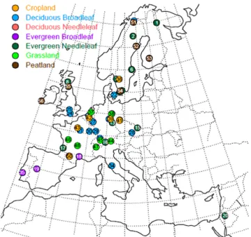
The European network of digital cameras currently covers over 50 flux sites across Europe (Fig. 1 and Table 1). Table 1 demonstrates that a diverse selection of commercially avail-able cameras are being used across the network. The cameras are installed in waterproof housing that is firmly attached to the flux tower some height above the top of the canopy. The cameras are generally orientated north, looking slightly down to the horizon to ensure that the majority of the image con-tains the vegetation of interest. Canopy images of the same scene are taken repeatedly each day, at a frequency that varies across the different sites from between 1 and 12 images per day and stored as 8-bit JPEG files (i.e. digital numbers
rang-Figure 1. Distribution of operational digital cameras at flux sites
across Europe; for further details, refer to Table 1.
ing from 0 to 255). The archived images used in the present analysis are all taken between 11:00 and 13:00 local time (LT). The camera setup is specific to each camera type but a common requirement to observe the seasonal colour fraction time series is to set the colour balance to “fixed” mode (on the Stardot cameras) or the white balance to “manual” mode (for the Nikon Coolpix cameras) (Mizunuma et al., 2013, 2014).
2.2 Image analysis
2.2.1 ROI selection and colour analysis
For each site, a squared region of interest (ROI) was selected from a visual inspection of the images. The ROI had to be as large as possible and common to all images of the same growing season, while including as many plants as possi-ble but no soil or sky areas. Image ROIs were then anal-ysed using the open-source image analysis software, Image-J (Image-J v1.36b; NIH, MS, USA). A customised macro was used to extract red–green–blue (RGB) digital number (DN) values between 0 and 255 (ncolour)for each pixel of the ROI,
and a mean value for all pixel values in a given ROI of each image was calculated. Various colour indices can be obtained from digital image properties (Mizunuma et al., 2011), but here we used only the chromatic coordinates, hereafter called colour fraction (Richardson et al., 2007):
colour fraction = ncolour/(nred+ngreen+nblue), (1)
where colour is either red, green or blue.
In the following we will thus refer to the “green fraction” as the mean green colour fraction for all pixels in the ROI, as
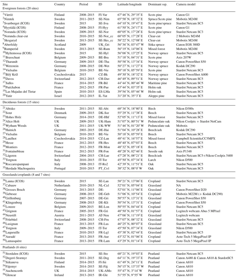
Table 1. List of participating sites in the European phenology camera network, period of camera operation, dominant vegetation cover and
camera model. NA denotes data that are not available.
Site Country Period ID Latitude/longitude Dominant ssp. Camera model
Evergreen forests (20 sites)
1Värriö Finland 2008–2015 FI-Var 67◦460N, 29◦350E Scots pine Canon G1
2Nimtek Sweden 2011–2015 SE-Nim 65◦580N, 18◦320E Spruce/Scots pine Mobotix M24M
3Svartberget (ICOS) Sweden 2015 SE-Sva 64◦100N, 19◦470E Scots pine/spruce Stardot Netcam SC5 4Hyytiälä (ICOS) Finland 2008–2015 FI-Hyy 61◦500N, 24◦170E Scots pine Canon G1 5Norunda (ICOS) Sweden 2009–2015 SE-Nor 60◦050N, 17◦280E Scots pine/spruce Stardot Netcam SC3 6Norunda clear-cut Sweden 2010–2015 SE-Nor_cc 60◦050N, 17◦280E Clear-cut 2 Mobotix M24M
7Skogaryd Sweden 2013–2015 SE-Sko_cc 58◦220N, 12◦080E Clear-cut Mobotix M24M
8Aberfeldy Scotland 2009 UK_Gri 56◦360N, 03◦470W Sitka spruce Canon EOS 300D
9Rumperöd Sweden 2013–2015 SE-Rum 56◦190N, 14◦060E Mixed forest Mobotix M24M
10Hyltemossa (ICOS) Sweden 2015 SE-Hyl 56◦060N, 13◦250E Norway spruce Stardot Netcam SC5
11Brasschaat Belgium 2009–2015 BE-Bra 51◦180N, 04◦310E Scots pine Axis 207W
12Tharandt Germany 2009–2015 DE-Tha 50◦580N, 13◦340E Norway spruce Canon PowerShot S50 13Wetzstein Germany 2008–2015 DE-Wet 50◦270N, 11◦270E Norway spruce Kodak DC290 14Vielsalm Belgium 2010–2015 BE-Vie 50◦180N, 05◦590E Scots pine Stardot Netcam SC5 15Bilý Kríž Czechoslovakia 2015 CZ-Bk 49◦300N, 18◦320E Norway spruce Canon PowerShot A800 16Davos Switzerland 2012–2015 CH-Dav 46◦490N, 09◦510E Norway spruce Stardot Netcam SC5 17Salles France 2014–2015 FR-Bil 44◦440N, 00◦460W Maritime pine Stardot Netcam SC5
18Puéchabon France 2012–2015 FR-Pue 43◦440N, 03◦350E Holm oak Stardot Netcam SC5
19Las Majadas del Tietar Spain 2010–2015 ES-LMa 39◦560N, 05◦460W Holm oak Stardot Netcam SC5
20Yatir Israel 2012–2015 IL-Yat 31◦200N, 35◦30E Aleppo pine Stardot Netcam SC5
Deciduous forests (15 sites)
21Abisko Sweden 2011–2015 SE-Abi 68◦360N, 18◦800E Birch Nikon D300s
22Sorø Denmark 2009–2015 DK-Sor 55◦290N, 11◦380E Beech Stardot Netcam SC5
23Hohes Holz Germany 2014–2015 DE-Hhf 52◦050N, 11◦130E Mixed forest Stardot Netcam SC5
24Alice Holt UK 2009–2015 UK-Ham 51◦070N, 00◦510W Pedunculate oak Nikon Coolpix + Stardot NetCam
25Wytham Woods UK 2011–2015 UK-WW 51◦460N, 01◦200W Pedunculate oak Mobotix
26Hainich Germany 2003–2015 DE-Hai 51◦040N, 10◦280E Beech/ash Kodak DC290
27Vielsalm Belgium 2010–2015 BE-Vie 50◦180N, 05◦590E Beech Stardot Netcam SC5
28Lanžhot Czechoslovakia 2014–2015 CZ-Lan 48◦410N, 16◦570E Mixed forest Campbell ScientificCC5MPX
29Hesse France 2012–2015 FR-Hes 48◦400N, 07◦030E Beech Stardot Netcam SC5
30Montiers France 2012–2015 FR-Mon 48◦320N, 05◦180E Beech Stardot Netcam SC5
31Fontainebleau France 2012–2015 FR-Fon 48◦280N, 02◦460E Sessile oak Axis P1348
32Lägeren Switzerland 2004–2015 CH-Lae 47◦280N, 08◦210E Beech/ash Stardot Netcam SC5+Nikon Coolpix 5400
33Torgnon Italy 2010–2015 IT-Tor 45◦500N, 07◦340E Larch Nikon D500
34Roccarespampani Italy 2008–2013 IT-Ro2 42◦390N, 11◦510E Oak Stardot Netcam SC5
35Herdade Machoqueira Portugal 2010–2015 PT_Co1 38◦320N, 08◦00W Oak Stardot Netcam SC5
Grasslands/croplands (8 and 7 sites)
36Lanna (ICOS) Sweden 2015 SE-Lan 58◦210N, 13◦060E Cropland Stardot Netcam SC5
37Cabauw Netherlands 2010–2015 NL-Ca1 52◦010N, 05◦040E Grassland NA
38Grosses Bruch Germany 2013–2015 DE- 52◦010N, 11◦060E Grassland Canon PowerShot D20
39Gebesee Germany 2008–2015 DE-Geb 51◦060N, 10◦540E Cropland Mobotix M22M (+ Kodak DC290)
40Grillenburg Germany 2007–2015 DE-Gri 50◦570N, 13◦310E Grassland Canon PowerShot S50 41Klingenberg Germany 2008–2015 DE-Kli 50◦540N, 13◦310E Cropland Canon PowerShot S50
42Lonzee Belgium 2009-2015 BE-Lon 50◦550N, 04◦440E Cropland Stardot Netcam SC5
43Grignon France 2005–2015 FR-Gri 48◦500N, 01◦570E Cropland Logitech webcam Abus 5 MPixel
44Neustift Austria 2011–2015 AT-Neu 47◦060N, 11◦190E Grassland Logitech webcam
45Früebüel Switzerland 2008–2015 CH-Fru 47◦070N, 08◦320E Grassland Stardot Netcam SC5
46Lusignan France 2013–2015 FR-Lus 46◦250N, 00◦070E Grassland Stardot Netcam SC5
47Torgnon Italy 2009–2015 IT-Tor 45◦500N, 07◦340E Grassland Nikon D500
48Laqueuille France 2010–2015 FR-Lq1 45◦380N, 02◦440E Grassland Stardot Netcam SC5
49Auradé France 2013–2015 FR-Aur 43◦320N, 01◦060E Cropland Aote-Tech 5 MegaPixel IP
50Lamasquère France 2013–2015 FR-Lam 43◦290N, 01◦140E Cropland Aote-Tech 5 MegaPixel IP
Peatlands (6 sites)
51Stordalen (ICOS) Sweden 2015 SE-Sto 68◦210N, 19◦030E Peatland Stardot Netcam SC5
52Degerö Stormyr Sweden 2011–2015 SE-Deg 64◦110N, 19◦330E Peatland Canon A480 & Canon A810 & StardotSC5
53Siikaneva Finland 2014–2015 FI-Sii 61◦490N, 24◦110E Peatland Canon A810
54Fäjemyr Sweden 2014–2015 SE-Fäj 56◦150N, 13◦330W Peatland Canon A810
55Auchencorth UK 2014–2015 UK-AMo 55◦470N, 3◦140W Peatland Canon A810
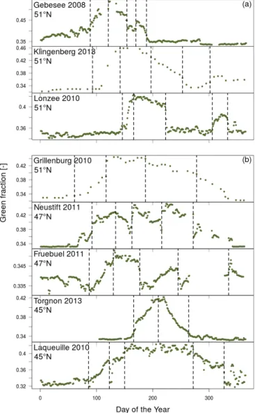
Figure 2. Green fraction time series for the broadleaf deciduous
forest, Hesse in France, the needleleaf evergreen forest Hyytiälä in Finland and the grassland Laqueuille in France, demonstrating the filtering and phenostage extraction approach used in our synthe-sis. Grey and black dots indicate raw and filtered data, respectively, while dashed vertical lines indicate the breakpoints extracted on the green fraction time series using the piecewise regression approach. At the bottom of each vertical line the 95 % confidence interval of the breakpoint dates is also shown.
opposed to the amount of pixels covered by vegetation in the entire image (Comar et al., 2012).
2.2.2 Data filtering procedure
Image quality is often adversely affected by rain, snow, low clouds, aerosols, fog and uneven patterns of illumination caused by the presence of scattered clouds. These influences often create noise in the trajectories of colour indices, and are an important source of uncertainty that can hamper the de-scription of canopy seasonal variations and the derivation of robust phenological metrics from colour index time series. To remove problematic images that were affected by raindrops, snow or fog from the digital photograph analysis, we used a filtering algorithm based on the statistical properties of the time series; we used two steps to filter the raw data. The first filter, based on the deviation from a smoothed spline fit as described in Migliavacca et al. (2011), was used to remove outliers. Thereafter, we applied the method implemented in Sonnentag et al. (2012), to reduce the variability of the colour fractions (Fig. 2).
2.2.3 Piecewise breakpoint change analysis
We used a piecewise breakpoint regression approach to ex-tract the main phenological events automatically, such as leaf emergence and senescence from the colour fraction time se-ries (Fig. 2). The procedure is implemented in the R package
strucchange (Zeileis et al., 2002, 2003) and is used to detect breaks in a time series by identifying points where the mul-tiple linear correlation coefficients shift from one stable re-gression relationship to another (Bai and Perron, 2003). The 95 % confidence intervals of the identified breakpoints were then computed using the distribution function proposed by Bai (1997). To obtain credible breakpoints in complex green fraction time series such as in highly managed sites (e.g. grazed or cut grasslands, multiple rotation crops) the pos-sibility of identifying numerous peaks or breakpoints (up to eight breaks) may be necessary. However, such a high num-ber of breakpoints would be excessive in natural ecosystems, and so we decided to set a maximum of five breakpoints per growing season, for both managed and natural ecosystems. We opted for a breakpoint approach over other commonly used methods to extract phenological transitions from time series (i.e thresholds, derivative methods) because it can be considered as more robust and less affected by noise in the time series (Henneken et al., 2013). This is particularly rel-evant for our application that encompasses a large data set consisting of many different camera set-ups (camera type, target distance, image processing).
2.2.4 Determining phenophases by visual assessment
In order to relate the breakpoint detection method to phe-nological phases we also visually examined images from broadleaf forest ecosystems for leafing out, senescence and leaf fall. Six pre-trained observers looked through the same daily images and used a common protocol to identify dates when (1) the majority of vegetation started leafing out (i.e. when 50 % of the ROI contains green leaves), (2) the canopy first started to change colour, first to non-green colours such as yellow and orange, in autumn and (3) the last day when a few non-green leaves were still visible on the canopy before the day the branches became bare.
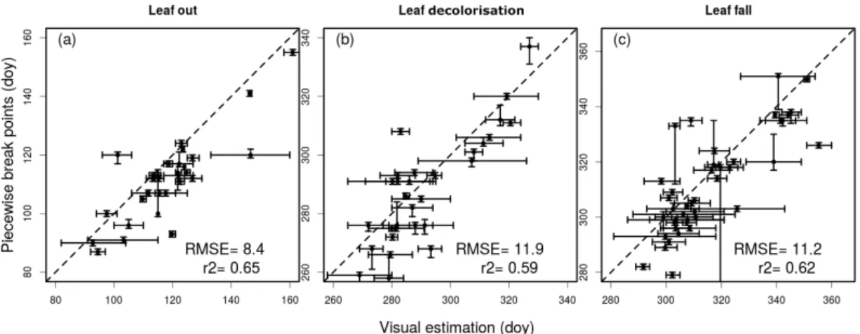
These visually assessed dates were then averaged across observers and compared to the relevant breakpoints, iden-tifying the same phenological stage. The leafing out phase was associated to the first automatically detected breakpoint, leaf senescence to the penultimate breakpoint and leaf fall to the last breakpoint. Based on this classification the key dates identified by the algorithm and visual inspection were consistently correlated with one another (Fig. 3). However, there was a tendency for the automatic algorithm to iden-tify all the phenological transitions before the visually as-sessed dates, by about a week. Also, visual inspections had larger standard deviations, especially during canopy senes-cence. Because of this systematic difference between the two methods, the breakpoints indicating the start of the growing season were in agreement with visually inspected dates to within 9 days only, and an even lower accuracy was found for leaf senescence and leaf fall (RMSE of 15.9 and 13.3 days, respectively). These RMSE values fall, however, within the range recently found by Klosterman et al. (2014) in a
simi-lar validation exercise performed with data from various US deciduous forests.
2.3 Radiative transfer modelling
To interpret the colour fraction time series produced by cam-eras in the network mechanistically, we combined the bi-directional radiative transfer model PROSAIL (Jacquemoud and Baret, 1990; Jacquemoud et al., 2009) with some ba-sic spectral properties of the photodetectors and the trans-mittances of the optical elements and filters used in the cam-eras, all combined into the so-called spectral efficiency of the RGB colour channels (GRGB, in DN W1, defined as the
dig-ital number per watt). This version of PROSAIL has been made available to the research community on the follow-ing repository (https://bitbucket.org/jerome_ogee/webcam_ network_paper). This version of PROSAIL is required to make the necessary link between the DN values measured by the camera sensors to the reflectances simulated by PRO-SAIL. It is also necessary to take into account the camera set-up and specific characteristics. Examples of these proper-ties are shown in Supplement (Figs. S1 and S2) for two types of camera from the network: (1) the Stardot NetCam CS5, in use at the majority of the European sites (Table 1) and the dominant camera used in the North American PhenoCam Network (http://phenocam.sr.unh.edu/webcam/) (Toomey et al., 2015) and (2) the Nikon Coolpix 4500, in use at two sites within the European camera network, and ca. 17 sites within the Japanese Phenological Eyes Network (PEN) (http: //pen.agbi.tsukuba.ac.jp/index_e.html) (Nasahara and Nagai, 2015).
The PROSAIL model combines the leaf biochemi-cal model PROSPECT (PROSPECT-5) that simulates the directional–hemispherical reflectance and transmittance of leaves over the solar spectrum from 400 to 2500 nm (Jacque-moud and Baret, 1990) and the radiative transfer model SAIL (4SAIL; Verhoef, 1984). The SAIL model assumes that dif-fusers are randomly distributed in space (turbid medium as-sumption) and thus may not be applicable for very clumped canopies such as sparse forests or crops (e.g. vineyards or-chards . . . ). Furthermore, the radiative transfer model as-sumes only one type of foliage, and therefore cannot deal well with species mixtures. However, for mixed forests, PROSAIL can still be used to interpret RGB signals if the ROI selected on the images is dominated by one single species. The version of the model used here (version 5B for IDL http://teledetection.ipgp.jussieu.fr/prosail/) requires 11 parameters from PROSAIL (leaf area, leaf angle, leaf mass and chlorophyll, carotenoid, water or brown pigment con-tents, hotspot parameter, leaf structural parameter and dry soil fraction, percentage of diffuse light) as well as geomet-rical parameters (sun height, view zenith angle and sun-view azimuthal difference angle). The percentage of diffuse light (ϕdiffuse)is necessary to calculate the amount of direct and
diffuse incoming radiation spectra at the top of the canopy
and is estimated here from observed incoming global radia-tion (Rg, in W m−2)using a procedure developed by Reindl
et al. (1990). The incoming radiation spectra at the top of the canopy are then estimated from Rg, ϕdiffuse and mean,
normalised spectra for direct (Idirect)and diffuse (Idiffuse)
ra-diation derived by François et al. (2002) using the 6S atmo-spheric radiative transfer model (Fig. S3). The 6S simula-tions performed by François et al. (2002) considered a vari-ety of aerosol optical thicknesses at 550 nm (corresponding to a visibility ranging from 8.5 to 47.7 km), water vapor con-tent (from 0.5 to 3.5 g cm−2, corresponding to most situations encountered in mid-latitudes), solar incident angle (from 0 to 78.5◦) and standard values for ozone, CO2and other
at-mospheric constituents but did not consider the presence of clouds. Therefore the derived spectra are only valid for cloud-free conditions and, following François et al. (2002), values of ϕdiffusebelow 0.5 were considered to represent such
cloud-free sky conditions. PROSAIL was then used to esti-mate the amount of light reflected by the canopy in the direc-tion of the camera for each wavelength E(λ) (W m−2nm−1)
from which we compute the RGB signals according to
IRGB=BRGB
Z λIR
λUV
GRGB(λ) E (λ)dλ, (2)
where λUVand λIRare the UV and IR cut-off wavelengths of
the camera sensor and filter (see Fig. S1) and BRGBis a
con-stant factor that accounts for camera settings (mostly colour balance) and was manually adjusted for each RGB signal and each camera/site using a few days of measurements out-side the growing season. The modelled RGB colour fractions were then computed in a similar fashion as in Eq. (1) but with
IRGBinstead of ncolour. In practice, GRBGis often normalised
to its maximum value rather than expressed in absolute units and for this reason, IRGB is not a true digital number, but
this has no consequence once expressed in colour fractions. Also, we are aware that the image processing of real (non-uniform) scenes is far more complex than Eq. (2) (Farrell et al., 2012) but from the preliminary results presented below, this simplistic formulation is robust enough to describe time series of average colour fractions over a large and fixed ROI, measured with different camera settings.
2.4 CO2flux analysis
A recent study by Toomey et al. (2015) demonstrated that the seasonal variability in daily green fraction measured at 18 different flux sites generally correlated well with GPP esti-mated from co-located flux towers over the season. However, they found that the correlation between daily GPP and daily green fraction was better for some plant functional groups (grasslands) than for others (evergreen needleleaf forests or deciduous broadleaf forests). Thus for some of the flux sites presented in Table 1, we also qualitatively related changes in vegetation indices to gross primary productivity (GPP) time series. Net CO2fluxes were continuously measured at
Figure 3. Relationship between the visual estimations of (a) leaf unfolding (b) leaf senescence and (c) leaf-fall day number compared to the
breakpoint day numbers estimated by the piecewise regression of green colour fractions for the broadleaf sites. Error bars represent the 95 % confidence interval, calculated from the mean of observation replicates (n = 6) for the visual estimation, and from the error of the piecewise regression coefficients for the breakpoint analysis.
each site using the eddy-covariance technique described in Aubinet et al. (2012). Level 4 data sets were both quality-checked and filled using online eddy-covariance gap-filling and flux-partitioning tools provided by the European flux database cluster (Lasslop et al., 2010; Reichstein et al., 2005). Full descriptions of the flux tower set-ups used to compare digital images and GPP are provided in Wilkinson et al. (2012) for Alice Holt (deciduous forest), Wohlfahrt et al. (2008) and Galvagno et al. (2013) for Neustift and Torgnon (sub-alpine grasslands), Vesala et al. (2010) for Hyytiälä (evergreen forest) and Aubinet et al. (2009) for Lonzee (cropland).
3 Results and discussion
3.1 Seasonal changes in green fraction across the
network
3.1.1 Needleleaf forest ecosystems
Differences in the seasonal evolution of canopy green frac-tions are presented for individual years at a selection of needleleaf forest flux sites spanning a latitudinal gradient of approximately ca. 30◦(31◦200–61◦500N) (Fig. 4 and Ta-ble 1). It was often difficult to automatically determine the start of the growing season for the coniferous sites, either be-cause of snow cover (noticeable changes in the colour sig-nals were often associated with the beginning and end of snow cover) or because of problems caused by the set-up of the camera (either too far away from the crown or the view contains too much sky). However seasonal changes in the amplitude of the canopy green fraction of needleleaf trees were generally conservative across sites and often displayed a gentle rise in green fraction values during the spring months (Fig. 4a) and a gentle decrease during the winter months. In
contrast, the deciduous Larix site in Italy showed a steep and pronounced start and end to the growing season that lasted approximately 5 months (Fig. 4b).
The main evergreen conifer species Pinus sylvestris L. and Picea abies L. exhibited different green fraction vari-ations during spring. In Picea species, new shoots contain very bright, light green needles that caused a noticeable in-crease in the green colour fraction during the months of May and June (Fig. 4, e.g. Tharandt and Wetzstein). In contrast, the new shoots of Pinus species primarily appeared light brown as the stem of the new shoot elongated (Fig. S4) and caused a small reduction in the green fraction, only de-tectable at a number of sites and years (Brasschaat in 2009, 2012; Norunda in 2011; Hyytiälä in 2008, 2009, 2010, 2012), followed by an increase in the green fraction values once nee-dle growth dominates at the shoot scale (Fig. 4 and S4).
The breakpoint analysis could identify a change in the green fraction when the canopy became consistently snow-free or covered in snow, but also when it experienced sus-tained daily mean air temperatures of above 0◦C (Fig. 5).
For instance, at the Finnish site Hyytiälä, the green fraction exhibited rapid changes during final snowmelt (day 18, bp1) and first snowfall (day 346, bp5 confirmed with visual in-spection of the images), but also around days 100–110 (bp2) as daily mean temperatures increased from −10◦C and sta-bilised for several days just above 0◦C and GPP rates in-creased (Fig. 5). Towards the end of the growing season sig-nificant changes in the green fraction were again detected by the piecewise regression approach, one around day 267 (bp3), coinciding with the period when minimum air tem-peratures began to fall below 0◦C and another around day 323 (bp4) coinciding with a short period of warmer tem-peratures (Fig. 5). Interestingly from the first breakpoints at the beginning of the year, day 115 (bp2) coincided with the onset of GPP, whereas towards the end of the season, day
Figure 4. A latitudinal comparison of filtered green fraction time
series for a selection of (a) evergreen and (b) deciduous needleleaf flux sites within the European phenology camera network. Vertical dashed lines indicate breakpoints that correspond to transitions in the green fraction over the growing season.
323 (bp4) coincided with a stable period of no photosynthe-sis (GPP = 0 gC m−2d−1)and a transient increase of daily mean temperature above 0◦C. However, the start of this sta-ble period with no photosynthetic uptake was not detected by a breakpoint. During this period the green fraction tracked fluctuations in the daily mean temperature. The recovery of biochemical reactions and the reorganisation of the photo-synthetic apparatus in green needles is known to be trig-gered when air temperature rises above 0◦C (Ensminger et al., 2004, 2008) and at about 3–4◦C at this particular site in Finland (Porcar-Castell, 2011; Tanja et al., 2003). Our results suggest that green fractions from digital images seem sensi-tive enough to detect these changes in the organisation of the photosynthetic apparatus of the coniferous evergreen needles as they acclimate to cold temperatures.
Figure 5. Time series of (a) daily temperature, daily PPFD (b) GPP (c) green fraction variations over the year with vertical solid lines
showing major breakpoint changes, identifying important transi-tions in the green fraction over the growing season at the Hyytiälä flux site in Finland during 2009.
3.1.2 Grassland and cropland ecosystems
Many land surface models still lack crop-related plant func-tional types and often substitute cropland areas with the char-acteristics of grasslands (Osborne et al., 2007; Sus et al., 2010). Our initial results from the European phenology cam-era network demonstrate the difficulty of teasing apart the seasonal and interannual developmental patterns as they are often complicated by co-occurring agricultural practices (e.g. cutting, ploughing, harvesting and changes in animal stock-ing density) (Fig. 6).
Overall we found that there was surprisingly little differ-ence between the onset dates of growth for most of the per-manent grassland sites, despite being located in very different locations across Europe; however, the onset of the green frac-tion signal was considerably delayed at the sub-alpine grass-land site in Torgnon compared with the other sites (Fig. 6). Torgnon also had the most compressed growing season of all the sites, encompassing a period of less than 100 days, some 100 days shorter than the other sites. These differences in growing season length between permanent grassland sites are caused by elevation (most grassland sites are situated at 1000 ± 50 m a.s.l., while the Italian site, Torgnon, is located at ca. 2160 m a.s.l.) that induced differences in temperature and snow cover and consequently the RGB signals.
Management practices such as the cutting of meadows (e.g. Neustift and Früebüel) and changes in animal stocking
Figure 6. A latitudinal comparison of filtered green fraction time
series for a selection of (a) cropland and (b) grassland flux sites within the European phenology camera network. Vertical dashed lines indicate breakpoints that correspond to transitions in the green fraction over the growing season.
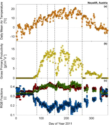
rate (e.g. Laqueuille) also created abrupt shifts in the RGB signals that could be distinguished from digital images. For example at the Neustift site in Austria, the meadow was cut three times during the 2011 growing season (days 157, 213, 272) causing pronounced drops in the blue fraction and to a lesser extent reductions in the green and red signal (Figs. 7 and S5). These meadow cuts were clearly identified in the green fraction time series by the breakpoint analysis (see bp3, bp4 and bp5 in Figs. 6, 7 and S5). In addition, flowering events were frequently strong drivers of the colour signals at the Neustift site. The vegetation at Neustift has been clas-sified as Pastinaco-Arrhenatheretum and is characterised by a few dominant grass (Dactylis glomerata, Festuca praten-sis, Phleum pratenpraten-sis, Trisetum flavescens) and forb
(Tri-folium pratense and repens, Ranunculus acris, Taraxacum officinale, Carum carvi) species. Flowering of these species caused gradual decreases in the red and green signals for sev-eral weeks prior to mowing (e.g. the yellow flowers of R. acris and T. officinale on days 131–156 (bp2), and the white flowers of C. carvi between days 176–212 see Fig. S5). In contrast, the blue signal tended to increase in strength during flowering periods, making the impact of the mowing events dramatic when they occurred (Fig. 7). If the piecewise re-gression algorithm was set to allow the detection of up to eight breakpoints at those sites, flowering events were of-ten identified as well as the mowing events but this made the detection of the start and end dates of the growing sea-son even more challenging using automated algorithms, as manual inspection of each breakpoint would be necessary to identify the dates of first leaf growth and leaf death. For ex-ample when eight breakpoints were observed in grassland ecosystems the first breakpoint was frequently caused by the start of the snow-free period, as opposed to the start of growth. Subsequent breakpoints typically indicated the phe-nology and management of the vegetation, particularly mow-ing and flowermow-ing, and suggest that a visual inspection of im-ages may still be necessary to clarify the nature and man-agement causes behind breakpoints in some grassland sites. Thus having the option to detect up to eight breakpoints or more could be an advantage for ecological studies on the phenology of flowering, pollination and community dynamic responses to environmental changes.
In addition, at some sites it was not always easy to dis-cern visually from images when a grassland started its first growth, as often fresh shoots are hidden by litter and dead material from the previous year. This particular problem may lead to a slight overestimation of the start date of growth and additionally lead to a potential temporal mismatch between GPP and green-up signals. For example at the subalpine site in Torgnon the green fraction and GPP peaked at the same time of year (bp2), but the onset of the green signal in spring lagged behind the onset of photosynthesis by about 7–10 days (Fig. 8). Given these results at Neustift, Torgnon and the other sites within the network, grassland green signals can provide additional information on the variations in GPP over the season and between years as suggested by Migliavacca et al. (2011) and more recently Toomey et al. (2015), but an underestimation of the growing season length may also occur using our automatic breakpoint detection approach.
As mentioned above, the use of grassland characteristics to describe the phenology of different crops is common in some land surface models. However, at the same site we can see that the start of the growth period for each different crop varies widely over commonly applied rotations. For example, at Lonzee in Belgium we found that for individual crop types such as potato and winter wheat the patterns of the green sig-nal were fairly similar between different years (Fig. 9). How-ever, we could still observe variations between years such as a slightly shorter green period for the potatoes in 2014
rela-Figure 7. Impact of (a) temperature, phenology and mowing
prac-tices on (b) GPP and (c) RGB colour fractions with solid vertical lines showing major breakpoint changes identifying important tran-sitions in the green fraction over the growing season for the alpine meadow flux site Neustift in Austria.
tive to 2010 or a slightly later start to the season for winter wheat in 2013 relative to 2011.
As huge areas of Europe are dedicated to the production of crops (326 Mha) and grasslands (151 Mha) (Janssens et al., 2003), and are known to be one of the largest European sources of biospheric CO2 to the atmosphere at a rate of
about 33 TgC yr−1 (Schulze et al., 2009), it is increasingly important that more field observations of developmental or phenological transitions are obtained to constrain the timing and developmental rate of plants in situ and improve model simulations. Our initial results from the European phenol-ogy camera network show that digital repeat photography may provide a valuable assimilation data set in the future for providing useful indicators of developmental transitions and agricultural practices (e.g. cutting, ploughing, harvesting and changes in animal stocking density).
3.1.3 Broadleaf forest ecosystems
Within the European phenology camera network, the ma-jority of broadleaf forest sites are deciduous and are iden-tified easily by the seasonal RGB signals they produce. Typ-ically the start of the temperate growing season coincides with a strong increase in the relative green fraction (Fig. 10). Across the network the timing of this spring green-up varies
Figure 8. Time series for the alpine grassland, Torgnon in Italy
demonstrating (a) the daily mean air temperature (b) the gross pri-mary productivity and (c) the calculated breakpoints for the green fraction using the piecewise regression approach. Vertical solid lines show major breakpoint changes, identifying important tran-sitions in the green fraction over the growing season
slightly with latitude, usually occurring first in the southern sites and moving north, with the British sites starting later than continental sites at similar latitude (for the same years data not shown) (Fig. 10). The end of the growing season, identified clearly as a decrease in the green signal, varied considerably across the network. The more continental sites such as the Hainich and Lägeren deciduous forests exhibited the shortest growing season lengths, whilst the oceanic and Mediterranean sites had far longer growing seasons. A high degree of variability in the timing for colour changes is com-monly found in autumn across temperate deciduous ecosys-tems (Archetti et al., 2008) despite the fact that, at least in the case of European tree species, changes in photoperiod and air temperature are usually considered as the main drivers of the colouration of senescent leaves (Delpierre et al., 2009a; Keskitalo et al., 2005; Menzel et al., 2006).
Interestingly, the evergreen broadleaf forests at the Mediterranean sites in Spain and France displayed similar RGB seasonal variations (Fig. 10b). However, the peak in the green fraction values were observed somewhat later in spring compared to those of the deciduous broadleaf sites. These maximum green fraction values are most probably linked to the production of new leaves that typically occurs at this pe-riod in Holm Oak (García-Mozo et al., 2007; La Mantia et al.,
Figure 9. Impact of crop management practices and crop rotation
on the green colour fractions over the growing seasons 2010–2014 for the agricultural flux site Lonzee in Germany.
2003). Interestingly, a strong decrease in the green fraction was observed prior to the peak at the Spanish site, Majadas del Tieter. Similar patterns in the NDVI time series have been observed around the same period, at the Puechabon site but for different years to the one studied here (2006–2008) (Soudani et al., 2012). This drop in NDVI was explained by the shedding of old leaves coinciding with the period of leaf sprouting in spring. However, on inspection of the Spanish site photos (Fig. S6) we found that the canopy during this period was covered in conspicuous male catkin-type flowers that appear yellow-brown in the images (Fig. 10). Thus, in the case of the Spanish site at least, the strong decrease in the green fraction seemed dominated by a male flowering event, in addition to the shedding of old leaves. In the case of the Puechabon site, visual inspection of the photos did not de-tect a strong flowering event, however, the camera is located slightly further away from the canopy, making it difficult to detect flowers easily by eye. However, phenological records maintained at the site indicate that the period between bp2
Figure 10. A latitudinal comparison of filtered green fraction time
series for a selection of (a) deciduous and (b) evergreen broadleaf forest flux sites within the European phenology camera network. Vertical dashed lines indicate breakpoints that correspond to transi-tions in the green fraction over the growing season.
and bp3 when the green signal slightly decreases, coincides with the start and end of the male flowering period, as well as leaf fall. In contrast, the signal between bp3 and bp4 indicates the period of leaf flushing for this year. Further studies com-paring NDVI signals with digital images should allow us to understand the observed variations in both signals better and their link to phenological events such as flowering and lit-terfall in evergreen broadleaves and how these vary between years in response to climate.
For broadleaf deciduous (and to some extent evergreen) species, our breakpoint approach also detected a significant decline in the green fraction a few weeks after leaf emergence and well before leaf senescence (Figs. 2 and 10). This pat-tern in the green fraction has also been observed for a range of deciduous tree species in Asia and the USA (Hufkens et
al., 2012; Ide and Oguma, 2010; Keenan et al., 2014a; Na-gai et al., 2011; Saitoh et al., 2012; Sonnentag et al., 2012; Toomey et al., 2015; Yang et al., 2014). In addition, this fea-ture has also been observed at the leaf scale using scanned images of leaves (Keenan et al., 2014a; Yang et al., 2014) and at the regional scale for a number of deciduous forest sites using MODIS surface reflectance products (Hufkens et al., 2012; Keenan et al., 2014a). The causes that underlie the shape and duration of this large peak at the beginning of the growing season remain unclear at present. Recent cam-era studies that have also measured either leaf or plant area index at the same time have found no dramatic reductions in leaf area during this rapid decline in the green fraction fol-lowing budburst (Keenan et al., 2014a; Nagai et al., 2011). At two of the deciduous sites within our network, Alice Holt and Søro (Fig. 10), daily photosynthetically active radiation (PAR) transmittance was also measured, providing a suitable proxy for changes in canopy leaf area. In both cases no de-crease in the leaf area index (LAI) proxy was detected during the decrease of the green signal shortly after budburst. If this decrease in the green signal after leaf growth is not caused by a reduction in the amount of foliage in most cases, it is likely associated with either changes in the concentration and phas-ing of the different leaf pigments or changes in the leaf angle distribution. These different hypotheses are tested in the next section.
3.2 Modelling ecosystem RGB signals
3.2.1 Sensitivity analysis of model parameters
Using the PROSAIL model as described above, with the camera sensor specifications of the Alice Holt oak site (see Fig. S1) we performed three different sensitivity analyses of the simulated RGB fractions to the 13 model parameters (Ta-ble 2). All sensitivity analyses consisted of a Monte Carlo simulation of between 2000 and 10000 runs each. For the first analysis the model was allowed to freely explore differ-ent combinations of the parameter space over the range of values commonly found in the literature and with no con-straints on how the parameters were related to each other (all parameters being randomly and uniformly distributed). The results from this initial sensitivity analysis indicated that the RGB signals were sensitive to four parameters: the leaf chlorophyll ([Chl]), carotenoid ([Car]) and brown contents (Cbrown)and the leaf structural parameter (N ) (see
Supple-ment, Fig. S7). In contrast, the simulated RGB signals were relatively insensitive to leaf mass (LMA), leaf water content (EWT) and, to some extent, to LAI (above a value of ca. 1). This sensitivity analysis also nicely demonstrates how mea-surements of NDVI made above canopies are most strongly influenced by LAI and to a slightly lesser extent by leaf pig-ment contents. Recent studies have also discussed whether changes in leaf inclination angle have a strong affect on the green fraction over the growing season (Keenan et al.,
2014a). Our simulations for two different camera view angles (one looking across the canopy and another looking down (results not shown)) indicate that this particular parameter did not have a strong impact on the RGB fractions (Fig. S7). The model also demonstrated that the impact of diffuse light had a negligible impact on the green fraction. In con-trast, an increase in the blue fraction alongside a decrease in the red fraction was observed as the percentage of diffuse light increased (Fig. S7). This result was anticipated given the different spectra prescribed for incoming direct and dif-fuse light (Fig. S3). However, it is also important to bear in mind that colour signals throughout this manuscript are ex-pressed as relative colour fractions (Eq. 1), and thus strong increases in one or more colour fraction, influenced by strong changes in a particular parameter (e.g. [Chl]. . . ), must also be compensated for by decreases in one or more of the other colour signals.
In a second sensitivity analysis conducted over the same time frame, we refined our assumptions on how certain pa-rameters were likely to vary with one another in spring dur-ing the green-up. For this, we fixed all parameters to val-ues typical for English oak during spring conditions (De-marez et al., 1999; Kull et al., 1999), except for LAI and the concentrations of chlorophyll and carotenoid. We then imposed two further conditions stating that (1) leaf chloro-phyll contents increased in proportion to LAI (i.e. the ratio of [Chl] / LAI was normally distributed) and (2) carotenoid and chlorophyll contents also increased proportionally (i.e. [Car] / [Chl] was normally distributed around 30 ± 15 %). This ratio between pigment contents is commonly found in temperate tree species. For example, Feret et al. (2008, see Fig. 3 therein) showed a strong correlation between the con-centrations of chlorophyll a/b and carotenoids for a range of plant types. This second sensitivity analysis revealed clearly how the RGB fractions would likely respond to LAI, chloro-phyll and carotenoid contents during the spring green-up (Fig. 11). Firstly, we observed that the RGB signals were more sensitive to LAI, [Chl] and [Car] when the analysis was constrained by our a priori conditions (compare panels from Fig. 11 with those of Fig. S7). In addition we found that the RGB fractions varied in sensitivity across the range of LAI variations typically found in deciduous forests. Most of the sensitivity in the green signal was found at very low val-ues of LAI (< 2), whereafter the signal became insensitive. In contrast, the NDVI signal remained sensitive throughout the full range of prescribed LAI values. For the range of likely [Chl] taken from the literature for oak species (Demarez et al., 1999; Gond et al., 1999; Percival et al., 2008; Sanger, 1971; Yang et al., 2014), our simulations indicated that the sharp increase in the green signals observed by the camera sensors during leaf out are mostly caused by an increase in [Chl]. More interestingly, and contrary to our previous anal-ysis where changes in [Chl] and [Car] were not correlated (compare the same panels in Fig. 11 with those presented in Fig. S7), this new analysis clearly shows that when [Chl]
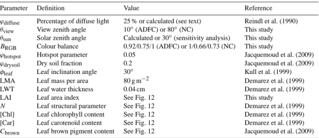
Table 2. List of parameters and values used to model the RGB signals at Alice Holt for the 2010 growing season. Camera-specific parameters
for the Stardot Netcam SC5 (NC) and the Nikon Coolpix (ADFC) are given separately.
Parameter Definition Value Reference
ϕdiffuse Percentage of diffuse light 25 % or calculated (see text) Reindl et al. (1990)
θview View zenith angle 10◦(ADFC) or 80◦(NC) This study
θsun Solar zenith angle Calculated or 30◦(sensitivity analysis) This study
BRGB Colour balance 0.92/0.75/1 (ADFC) or 1/0.66/0.73 (NC) This study
ϕhotspot Hotspot parameter 0.05 Jacquemoud et al. (2009)
ϕdrysoil Dry soil fraction 0.2 Jacquemoud et al. (2009)
φleaf Leaf inclination angle 30◦ Kull et al. (1999)
LMA Leaf mass per area 80 g m−2 Demarez et al. (1999)
LWT Leaf water thickness 0.04 cm Demarez et al. (1999)
LAI Leaf area index See Fig. 12 This study
N Leaf structural parameter See Fig. 12 Demarez et al. (1999)
[Chl] Leaf chlorophyll content See Fig. 12 Demarez et al. (1999)
[Car] Leaf carotenoïd content See Fig. 12 Demarez et al. (1999)
Cbrown Leaf brown pigment content See Fig. 12 Jacquemoud et al. (2009)
reached ca. 30 µg cm−2, the green signal begins to respond negatively to a further increase in [Chl]. This is because in this simulation, an increase in [Chl] is accompanied by an increase in carotenoids and the green fraction responds neg-atively to an increase in [Car] (Figs. 11 and S7). Another interesting feature of this sensitivity analysis is how the de-pendence of NDVI on pigment content was greater when we imposed the two constraints described above. This investi-gation with the PROSAIL model therefore suggests that the sharp reduction in the green fraction commonly observed af-ter budburst in deciduous forests is mostly driven by an in-crease in leaf pigment concentrations.
3.2.2 Modelling seasonal RGB patterns mechanistically
Using the PROSAIL model and a few assumptions on how model parameters varied over the season (Table 2, Fig. 12) we investigated the ability of the PROSAIL model to simu-late seasonal variations of the RGB signals measured by two different cameras installed at the Alice Holt site. For this, a proxy for seasonal variations in LAI was obtained by fitting a relationship to values of LAI estimated from measurements of transmittance as described in Mizunuma et al. (2013), while the expected range and seasonal variations of [Chl], [Car], Cbrownand N were estimated from several published
studies on oak leaves (Demarez et al., 1999; Gond et al., 1999; Percival et al., 2008; Sanger, 1971; Yang et al., 2014), as summarised in Table 2. We also manually adjusted the parameter BRGB in Eq. (4) to match the RGB values
mea-sured by the camera during the winter period prior to bud-burst (highlighted by the grey bar in Fig. 12).
Using this simple model parameterisation, the model was able to capture the seasonal pattern and absolute magni-tude of the three colour signals relatively well, including the spring “green hump” (Fig. 12). As anticipated from our
sensitivity analysis (Fig. 11) we found that at the beginning of the growing season the initial rise in the green signal is dominated by small changes in LAI and [Chl], whilst the small decrease in the green signal that follows is most likely caused by the further increase of [Chl] and [Car]. This period is also characterised by a strong decrease in the red signal and a strong increase in the blue fraction that distinguishes it clearly from the effect of changes in LAI (as blue and green signals remain constant at LAI > 2). This relationship is ex-pected as the absorption by chlorophyll and carotenoids are not the same in all wavelengths (Feret et al., 2008, see Fig. 8 therein) and can account for most of the observed colour sig-nal trends. Interestingly the maximum green sigsig-nal observed by the camera coincides with the time when LAI reached half of its maximum value (dotted line on graphs), rather than when [Chl] is maximum. This theoretical result is consistent with pigment concentration data from other recent studies (Keenan et al., 2014a; Yang et al., 2014). Our analysis also indicates that the time when maximum [Chl] and/or [Car] is attained coincides more with the end of the green hump (i.e. several weeks after the peak in the green fraction) and also corresponds to when ecosystem GPP reaches its maximum. Recent pigment concentration measurements performed in the same forest canopy in 2012 and 2013 seem to confirm this theoretical result (data not shown).
Our observations across the deciduous forest sites of the network also highlight a second strong hump in the red and blue signals towards the end of the growing season linked to senescence of the canopy. This autumnal change in colour fractions starts with a decrease in both the green and blue signals and a strong increase in the red signal. To under-stand this combined signal we conducted a third sensitiv-ity analysis with the model. In this Monte Carlo simulation we maintained all parameters of the model constant except those likely to be important during autumn, mainly LAI,
0W - 51N - sun=60 NC camera 0.40 0.50 0.60 0.70 0.80 0.90 NDVI fr a c tion 0.15 0.20 0.25 0.30 0.35 0.40 B lue fr act io n 0.30 0.35 0.40 0.45 Gr ee n f ra c ti on 0.30 0.35 0.40 0.45 Re d f ra c ti on 1 2 3 4 5 LAI [m2 m-2] 0 20 40 60 80 100 Fr eq uen cy 0W - 51N - sun=60 NC camera 0 20 40 60 Chl [g cm-2] 0W - 51N - sun=60 NC camera 0 5 10 15 20 25 Car [g cm-2]
Figure 11. Sensitivity of modelled RGB fractions and NDVI for
the NetCam camera at the Alice Holt deciduous broadleaf forest, as predicted by the PROSAIL model and constrained by Chl : Car and Chl : LAI ratios (see text and compare to those in Fig. S7). All other parameters are set to standard budburst values and the solar
eleva-tion is fixed at 60◦. The NDVI is computed using the camera view
angle and the same wavebands as for MODIS NDVI (545–565 nm for red and 841–871 nm for near infrared). The bottom panel rep-resents the frequency of estimates for a given value of a particu-lar parameter. One can see that compared with Fig. S7 there are more likely to be values skewed to the lower pigment concentra-tions with our constraints compared with the no-constraints analysis of Fig. S7.
[Chl], [Car], Cbrownand N (Table 2). Correlations between
[Chl] and LAI on the one hand, and [Car] and [Chl] on the
Figure 12. Time series of modelled leaf chlorophyll (Chl),
carotenoid (Car) and brown pigment (Cbrown)contents, leaf
struc-tural parameters and modelled LAI used to predict RGB colour fractions at the Alice Holt broadleaf deciduous forest for the Net-cam Net-camera and the 2010 growing season. Other parameters are as in Table 2. Proxy LAI estimates and measured RGB frac-tions from camera images are also shown for comparison, as well as measured daily gross primary productivity. Cloud-free
condi-tions (ϕdiffuse< 0.5) are distinguished from cloudy conditions using
closed symbols. The thick grey horizontal bar indicates the period
used to adjust BRGB (see text). The IDL code and data required
to generate these figures can be downloaded from the repository (https://bitbucket.org/jerome_ogee/webcam_network_paper).
other hand were kept as for the sensitivity analysis shown in Fig. 11.
The results from this third sensitivity analysis suggest that the start of the autumnal maximum is most likely caused by a reduction in [Chl] and [Car] of the foliage and a simul-taneous increase in the structural parameter N and brown
pigment concentration (Fig. 12). The degradation of green chlorophyll pigments in autumn has been observed in oak and other temperate forest species before. Interestingly, the rate of degradation in [Chl] and [Car] during the autumn breakdown is not always proportional and can often lead to a transient increase in the [Car] / [Chl] that allows the yellow carotenoid pigments to remain active as nutrient remobili-sation takes place. Leaves of temperate deciduous broadleaf forests in Europe have an overall tendency to yellow in au-tumn and eventually turn brown before dropping (Archetti, 2009; Lev-Yadun and Holopainen, 2009). This subsequent browning of the foliage is the likely cause for the sharp de-crease in the red signal and inde-crease in the blue signal around day 325 (Fig. 12). Visual inspection of the digital images confirmed this was the case and was reflected in the mod-elling with the increase in Cbrown, the only parameter that
can reconcile the strong reduction in the red signal and the increase in blue strength observed (Fig. 13). Thereafter, re-ductions in LAI may also contribute further to this trend as leaves fall from the canopy.
Results shown in Figs. 11–13 have been obtained using spectral properties of the Stardot camera, that we obtained directly from the manufacturer (D. Lawton, personal com-munication, 2012). However, at Alice Holt, both a Stardot camera and a Nikon camera have been operating since 2009 (Mizunuma et al., 2013). Using a similar approach but with the Nikon camera, we then tested the idea that colour frac-tions seen by this other camera would also suggest similar variations in leaf pigment and structural parameters over the season. Spectral characteristics of the Nikon Coolpix 4500 were characterised at Hokkaido University in Japan and are shown in the Supplement (Fig. S2). We then used these cam-era specifications and the same parameterisation of canopy structural properties (LAI and N ) and leaf pigment concen-trations as the those used in Fig. 12. We also manually ad-justed BRGBusing the same procedure as for the Stardot
cam-era.
From this camera comparison we found that, in order to match the independent RGB camera signals with the same radiative transfer model, only the value of Cbrownduring the
growing season had to be adjusted (Fig. S8). On inspection of the camera images this may be justified as the scenes and ROI captured by each camera are very different despite looking at the same canopy, as the Stardot looks across the canopy, whilst the Nikon has a hemispherical view looking down on the canopy. Based on the need for different levels of Cbrown,
it is suggested that more brown (woody material) occupies the ROI of the Stardot camera during the vegetation period compared with that in the Nikon image, as confirmed in the images. Besides this difference in Cbrown, the same model
parameterisation reasonably captured the seasonal features of all three colour signals.
0W - 51N - sun=60 NC camera 0.40 0.50 0.60 0.70 0.80 0.90 NDVI fr a c tion 0.15 0.20 0.25 0.30 0.35 0.40 Bl ue fr act io n 0.30 0.35 0.40 0.45 Gr ee n f ra c ti on 0.30 0.35 0.40 0.45 Re d f ra c ti on 1 2 3 4 5 LAI [m2 m-2 ] 0 20 40 60 80 100 Fr eq uen cy 0W - 51N - sun=60 NC camera 0 20 40 60 Chl [g cm-2 ] 0W - 51N - sun=60 NC camera 0 5 10 15 20 25 Car [g cm-2 ] 0W - 51N - sun=60 NC camera 1 2 3 4 5 Cbrown 0W - 51N - sun=60 NC camera 1.5 2.0 2.5 3.0 N
Figure 13. Results from the PROSAIL sensitivity analysis as
per-formed in Fig. 12 except that the leaf brown pigment (Cbrown)and
structural paramer (N ) are now allowed to vary independently of the other parameters, as expected during senescence.
3.3 Technical considerations for the camera network
As demonstrated in this paper and elsewhere (Keenan et al., 2014a; Migliavacca et al., 2011), researchers are now explor-ing the link between canopy colour signals and plant physi-ology in order to maximise the utility of this relatively inex-pensive instrument. However, for this step to proceed further, the network should address several technical considerations. Firstly, the digital cameras in our European network are currently uncalibrated instruments unlike other commonly used radiometric instruments. In addition, these cameras are deployed in the field and are often exposed to harsh environ-mental conditions. Thus their characteristics may drift over time. For example although the CMOS sensors (commonly found in the cameras of our network) do not age quickly over periods of several years, the colour separation filters on the sensor plate may age after time because of UV exposure. Most commercial cameras already contain UV filter protec-tion and in addiprotec-tion they are protectively housed from the el-ements and sit behind a glass shield that protects the camera